Effect of Pore Structure on Soot Deposition in Diesel Particulate Filter

Abstract

Nowadays, in the after-treatment of diesel exhaust gas, a diesel particulate filter (DPF) has been used to trap nano-particles of the diesel soot. However, as there are more particles inside the filter, the pressure which corresponds to the filter backpressure increases, which worsens the fuel consumption rate, together with the abatement of the available torque. Thus, a filter with lower backpressure would be needed. To achieve this, it is necessary to utilize the information on the phenomena including both the soot transport and its removal inside the DPF, and optimize the filter substrate structure. In this paper, to obtain useful information for optimization of the filter structure, we tested seven filters with different porosities and pore sizes. The porosity and pore size were changed systematically. To consider the soot filtration, the particle-laden flow was simulated by a lattice Boltzmann method (LBM). Then, the flow field and the pressure change were discussed during the filtration process.

1. Introduction

It is well known that the combustion generated soot is harmful to our human health, because it is certain toxic and has carcinogenic effect [1,2]. Especially, the diesel soot in exhaust gas mainly consists of solid particles, which are generally called particulate matter (PM). Theoretically, the soot appears due to incomplete combustion in the diesel engine. Most of soot particles exist both in the ranges of 0.1 to 0.3 μm, and 0.005 to 0.05 μm. The smaller particles can be transported to the deeper region of our lung tissues densely packed with alveoli [3]. Additionally, it would contribute to environmental degradation and global warming. Therefore, in many countries including Japan, the stricter regulations on the emission of PM have been set, such as the so-called Euro VI in recent emission standards.

Nowadays, in the after-treatment of diesel exhaust gas, a diesel particulate filter (DPF) has been used to reduce nano-particles of the diesel soot. To trap these particles, the filter is placed in the exhaust stream of the diesel engine. Its filtration technique is very simple. When the diesel soot in the exhaust gas goes through the ceramic porous wall of DPF, the diesel soot is trapped inside the filter wall. The filtration efficiency is over 99% [4,5,6]. However, as there are more particles inside the filter, the pressure which corresponds to the filter backpressure increases. Resultantly, the fuel consumption rate is worsened, together with the abatement of the available torque. Thus, in order to fit stricter regulations in the future, a filter with lower backpressure would be needed. To achieve this, it is necessary to utilize the information on the phenomena including both the soot transport and its removal inside the DPF, in compliance with the optimal operating conditions.

Unfortunately, in experiments, less data was obtained, because we could measure only the exhaust gas temperature, species component, and the pressure drop across the filter. For the better design of the DPF with efficient filtration and more durability, we need to conduct a numerical simulation on the exhaust gas flow with soot particles in the DPF. However, in conventional computational code, it would still be difficult to take the filtration process into consideration, because we must set the complex boundary conditions at the very concave and convex filter substrate. Quite recently, a lattice Boltzmann method (LBM) has been widely used for alternative fluid simulation [7,8,9,10,11,12,13]. Many research papers have been published, especially for simulations in porous media [14,15,16,17,18]. In our previous studies, we have made great progress for developing the numerical approach of the soot particle-laden diesel exhaust gas by LBM [8,9,10,11]. So far, we could discuss the particle filtration together with pressure rise, which appears in the real usage of the diesel filter. Moreover, mass and heat transport was modelled for the filter regeneration process, by which it could be possible to discuss the soot oxidation in the catalyzed filter [7,10,11,19].

In this study, to obtain useful information for optimization of the filter structure, we test a variety of filter structures with different porosity and pore size. The size and geometry of commercialized DPF products are referred to the real filter. To change the porosity and pore size systematically, the porous structure of the filter substrate is formed by simulation, where two-phase flow is applied based on our previous approach [20,21,22]. Then, the flow with soot deposition is simulated for the PM trap inside the different filters.

2. Numerical Model

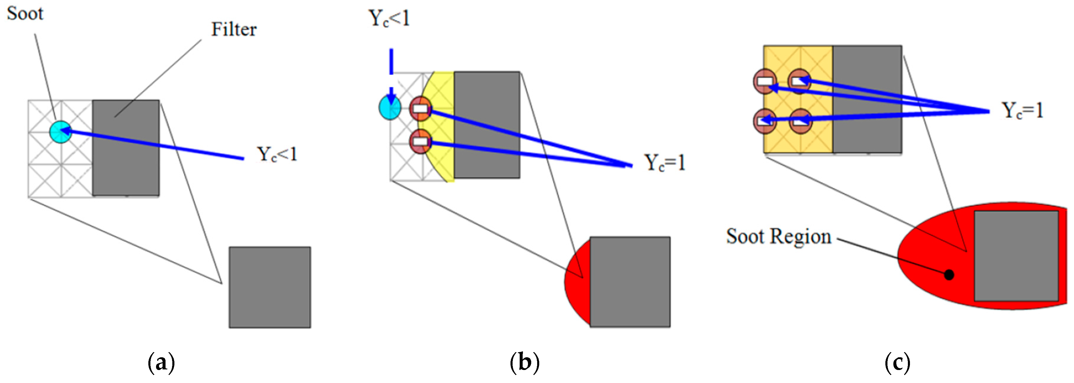
2.1. Soot Deposition Model

We simulate the soot deposition in DPF by the LBM. The detailed information on the principles of LBM is found in other references [13,23]. Recently, the LBM has been used as a diesel soot trap in national laboratories and universities [24,25,26]. One of our unique procedures is that we use CT data of inner structure of DPF to realize the real fluid flow in the filter. In our last several papers [7,8,9,10,11], we have simulated the soot trap and regeneration of the filter. Due to the computational costs, it must be impractical to consider the real geometry of the diesel soot, because it is carbonaceous agglomerates with several-micrometer primary soot [3,27,28]. For an alternative approach, our model only describes the soot mass fraction in the gas phase, by which the growth of the deposited soot layer is numerically reproduced. Then, we do not have to consider the real geometry of the diesel soot. Uniquely, the soot deposition probability on the filter substrate, P_D, has been proposed previously [9,11]. Our collaborators, including an automobile company and a Japanese national institute, estimated the value of the soot deposition probability, and it was 0.002 in the case of the cordierite filter [29]. It should be noted that, in the soot deposition region, the soot has many micro-pores. The flow can pass through the soot region. In our soot deposition model, the pressure rise across the soot region was included by the friction force in the fluid [8,25].

The procedure of the soot deposition process is explained in Figure 1. At a given time (time step IT₁), the soot arrives around the filter substrate, corresponding to one lattice node in the Figure 1a. As mentioned before, only the soot mass fraction of P_D is deposited, while that at (1 − P_D) is not trapped and is rebounded into the original gas flow. As the calculation proceeds, the sum of the soot concentration at the lattice point is increased. At some point, the mass fraction of soot becomes united at the time step, IT₂. Then, this node is treated as the solid phase of the soot layer, instead of the gas phase. At the next time step, IT₂ + 1, the soot deposition region is moved to one node next to the original boundary. In this way, the layer of the soot region is thickened.

2.2. Porous Structure of DPF

In this section, we explain the porous structure used in the simulation. Several porous structures with different porosities and pore sizes were produced numerically [20,21,22]. The porosity and pore size were determined by the degree of two-phase separation. Using each of these structures as a part of the filter wall, the performance of the soot filtration was examined. The spatial resolution of the filter substrate was 1 μm, and the size of each filter was 100 (x) × 80 (y) × 80 μm (z).

Table 1. Filter properties of seven filters.

Filter No.	Porosity, ɛ (−)	Upstream Pore Size D1 (μm)	Downstream Pore Size, D2 (μm)	Average Pore Size, D (μm)	Initial Pressure Drop, p0 (Pa)
1	0.49	18	18	18	33.1
2	0.49	11	11	11	82.4
3	0.49	31	31	31	12.2
4	0.42	18	18	18	41.7
5	0.61	18	18	18	24.6
6	0.49	28	15	19	34.5
7	0.49	15	28	20	36.5

shows seven porous structures with different porosity and pore size.

In the case of Filters 6 and 7, their filter property was changed inside the filter. That is, the inner structure was divided by two regions (upstream and downstream regions). Filters 6 and 7 have the same porosity as that of Filter 1, but their pore size is changed at upstream and downstream regions. More precisely, a filter substrate in which the pore diameter of upstream region (D₁) was set to be 28 μm and the pore diameter of downstream region (D₂) was set to be 15 μm was Filter 6. A porous material in which the pore diameter of upstream region (D₁) was 15 μm and the pore diameter of downstream region (D₂) was 28 μm was Filter 7.

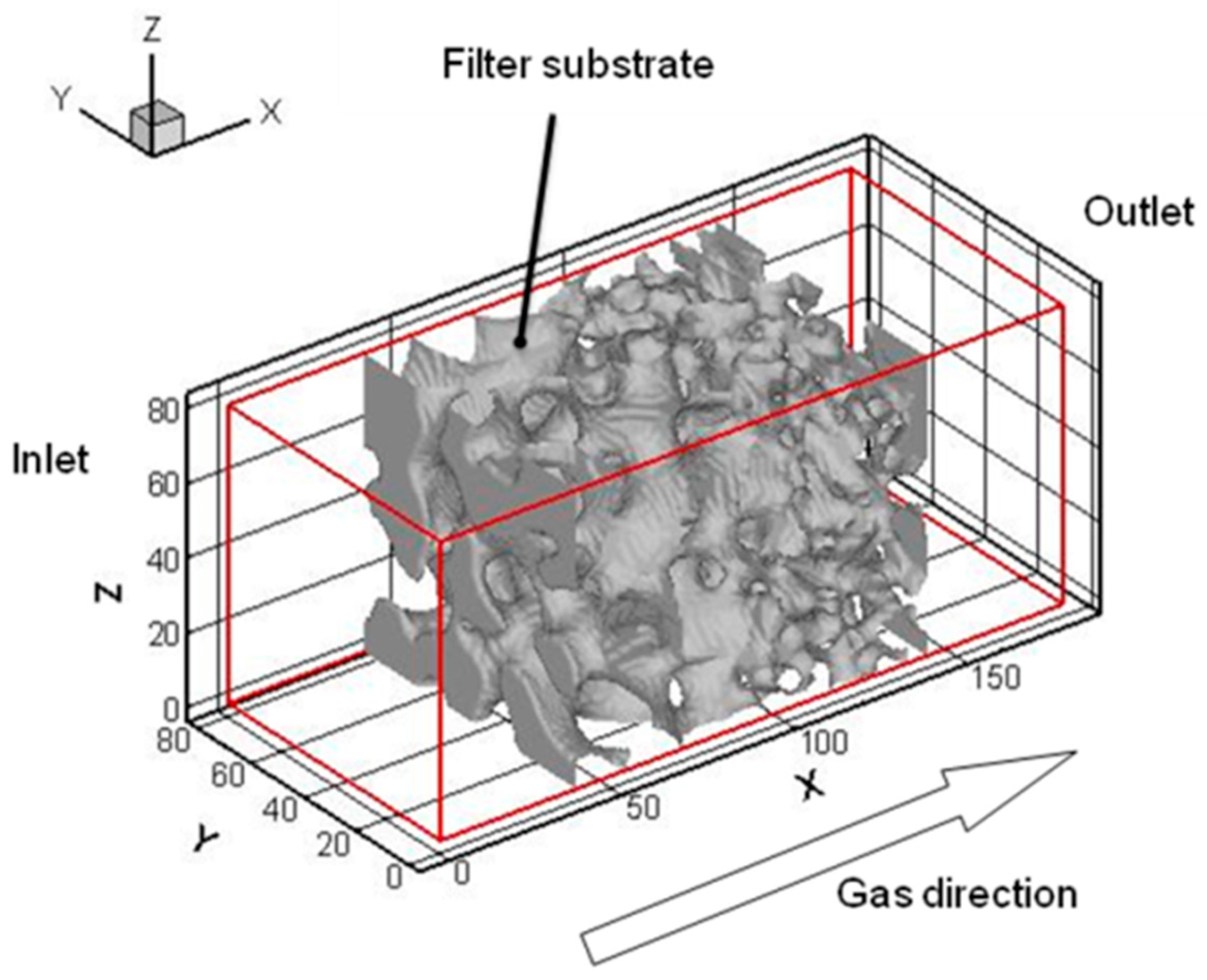
2.3. Numerical Domain

In this study, the filter properties of porosity and pore size were assumed to be those of the real DPF [20,21,22]. Figure 2 shows the calculation domain with Filter 6. The grid size is 1 μm in the simulation. The coordinate x is the flow direction passing through the filter wall. The filter of 112 (x) × 80 (y) × 80 μm (z) is set at the center. Then, the total calculation domain is 180 (x) × 80 (y) × 80 μm (z), including inlet and outlet zones of 34 μm. For reference, slice images of Filters 1, 6, 7 are shown in Figure 3.

As for the boundary conditions, the same approach was taken [7,8,9,10,11]. At filter inlet, the exhaust gas containing soot was evenly flowed from upstream. The non-dimensional variables including the Reynolds number were used to consider the similarity in LB space [30]. The flow velocity at the inlet (U_in) was 1 cm/s, which was the value in experiments [29]. The temperature of exhaust gas at the inlet (T_in) was set at 350 °C. The exhaust gas was composed of soot, oxygen, and nitrogen. The oxygen concentration was 10% in the volume fraction (X_O2), and the soot mass fraction was 0.1 (Y_c,in). The velocities were set at u = U_in, v = 0, and w = 0. At the four side walls, the slip boundary was adopted based on the assumption of symmetry. At the outlet, the pressure was constant (atmospheric pressure), and the gradient of scalars, such as temperature and mass fraction, were set to be zero. The non-slip boundary was adopted at the surface of the filter substrate, corresponding to the wall boundary condition [31].

3. Results and Discussion

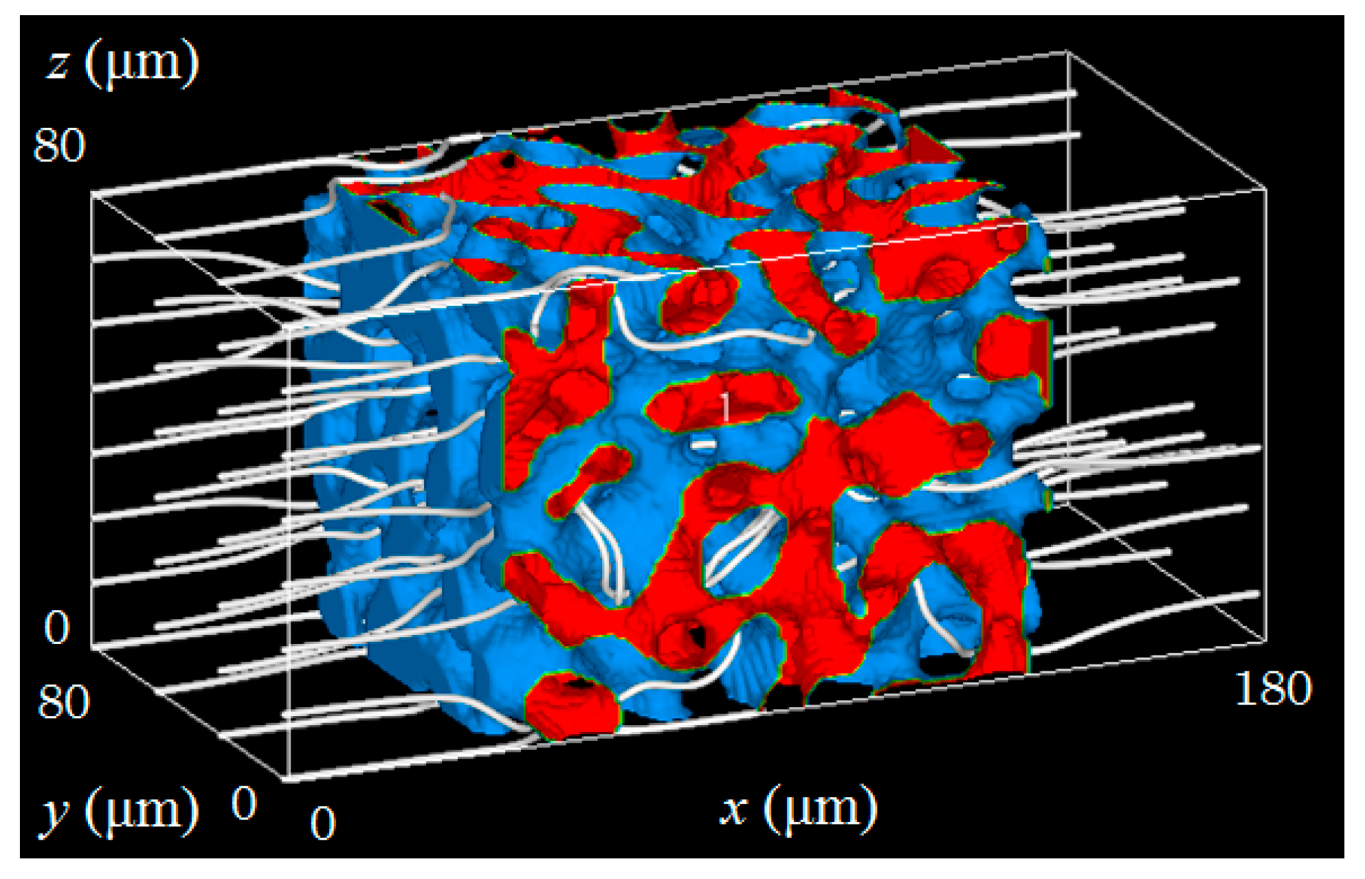
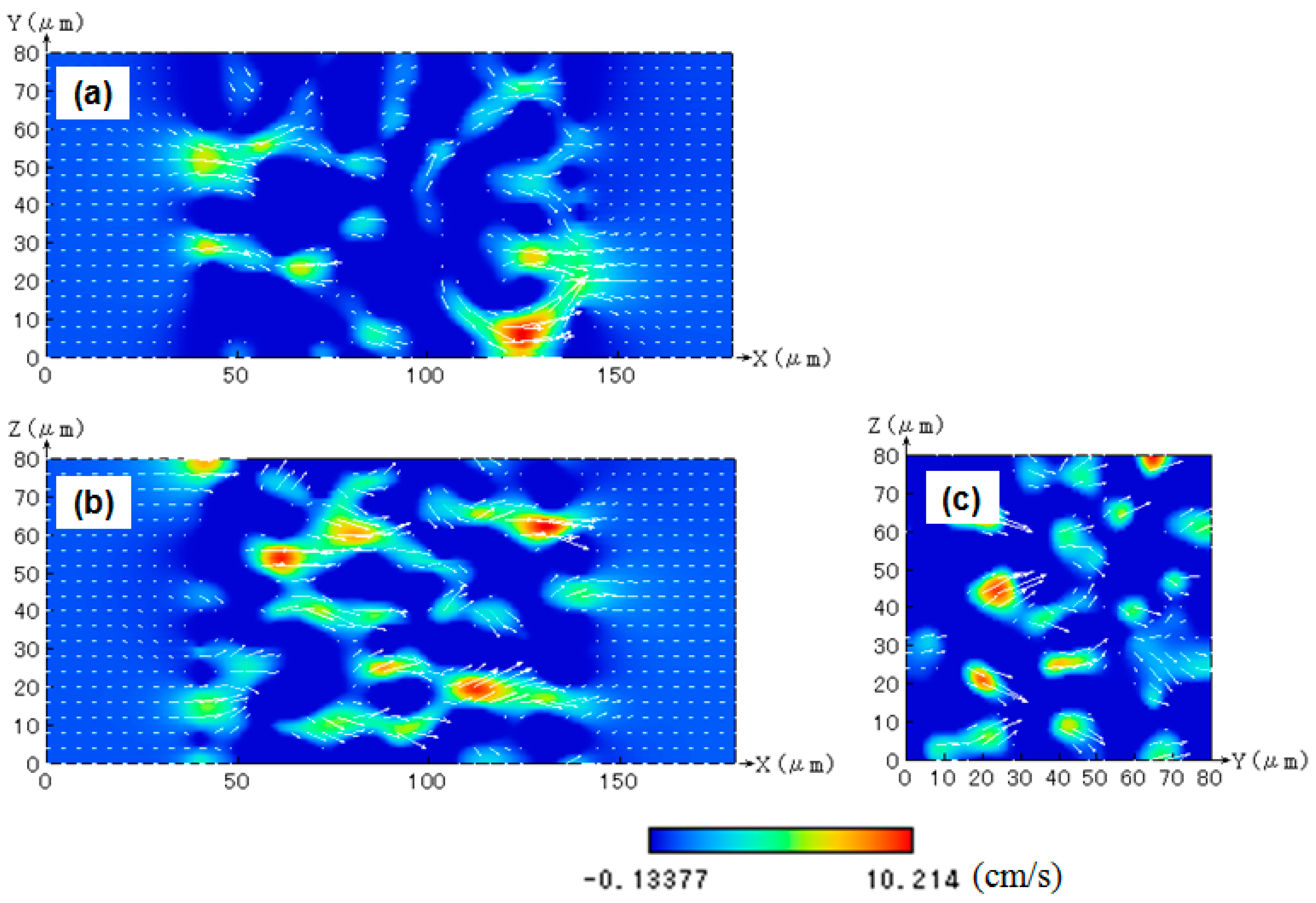
3.1. Flow Field and Pressure Drop without Soot Deposition

First of all, only the flow field is examined, because the flow passing through the filter could be much different by changing the filter property. Figure 4 shows the flow field with a streamline inside Filter 1. In this section, all results are profiles at steady state. Since the filter has a porous structure, the complex flow pattern is observed. Additionally, there are a number of flow paths across the filter wall. It is expected that these flow paths are gradually changed with soot deposition, resulting in an increase of filter backpressure.

Figure 5 shows the distributions of velocity in (a) x-y plane, (b) x-z plane, (c) y-z plane. These are the cross section at the center of the filter 1. The velocity in x-direction is shown by color bar. Although the inflow velocity is only 1 cm/s, the maximum velocity inside the filter is over 10 cm/s. That is, the filtration velocity could be 10 times larger than the inflow velocity. It is due to the fact that the flow is forced to pass through the narrow space between filter substrates, and the flow is largely accelerated. In some areas, the flow recirculation with negative velocity is observed.

Figure 6a shows the distribution of pressure which is an averaged value in each y-z plane. It should be noted that the difference of the pressure between the inlet and the outlet is the initial pressure drop (filter backpressure), which is shown in Table 1. Inside the filter, a constant pressure drop along the flow direction (x) is observed, because these porous structures are uniform. It is found that the initial pressure drop is the greatest in Filter 2, in which the average pore size is small. On the other hand, Filter 3 shows the smallest pressure drop, in which the average pore size is large. The initial pressure drop of Filter 4 is slightly greater than that of Filter 1, simply because the porosity is smaller. Similarly, the initial pressure drop of Filter 1 is greater than that of Filter 5. Thus, the initial pressure drop is determined by the porosity and pore size.

However, as shown in Figure 6b, for Filters 6 and 7, a linear decrease in pressure is not observed even if the porosity of these filters has almost the same value as that of Filter 1. This is because the pore size is changed inside the filter. In the case of Filters 6 and 7, the flow pattern is largely changed along the boundary at the center of the calculation domain. Expectedly, when the pore size in downstream region is smaller, the flow is difficult to pass through, resulting in the higher pressure drop. On the other hand, in Filter 7, the pressure change is smaller in the downstream region where the pore size is larger. However, the initial pressure drop is almost the same for Filters 1, 6, 7, because the averaged pore size is almost the same. Needless to say, the behavior of soot deposition could be different, which will be discussed in the next section.

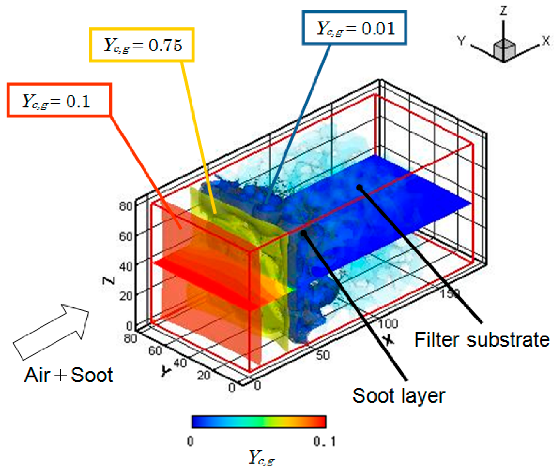
3.2. Soot Deposition for Filtration

In this section, we analyze the phenomena in which soot is deposited inside the filter wall. Different from the previous section, the flow field is always changed, because both pore size and porosity could be changed due to soot deposition. Then, we investigate the time-dependent relationship between the amount of soot deposition and the pressure drop. Figure 7 shows the three-dimensional distribution of soot mass fraction in the gas phase in Filter 1 at t = 15 s, where the time, t, is counted right after the simulation starts. At this point, a part of the filter surface is covered with a thin soot layer. As seen in this figure, a large reduction of soot in gas phase is observed around the inlet, and consequently, the concentration of soot is almost zero at the outlet. In this case, most of soot is deposited inside the filter wall, which corresponds to the depth filtration.

Next, three-dimensional soot layer at t = 15, 20, and 35 s is shown in Figure 8. For further visualization, two-dimensional images in x-y plane (z = 40 μm), corresponding to the slice images of the soot layer, are shown in Figure 9. These are also the profiles at t = 15, 20, and 35 s. It is observed that, initially, soot is deposited inside the filter wall, and then, pores are covered with soot on the filter surface. That is, pores on the filter surface are gradually clogged with soot, forming a soot deposition layer (called soot cake) on the filter surface. Once the soot cake is formed, all of soot is trapped by this soot layer, which is called the surface filtration [5]. Therefore, the transition between the depth filtration and the surface filtration is realized in the simulation [8]. This transition is observed in all seven filters in Table 1.

In general, when the diesel soot in exhaust gas is collected using DPF, the difference in the pressure before and after the filter, corresponding filter backpressure, increases. This pressure drop is known to change according to the location where the soot deposits inside the DPF. Figure 10 shows the time-variation of deposited soot mass and the pressure drop in Filter 1. The deposited soot mass is shown based on the value of soot mass divided by the total filter volume, which is a well-known property when the filter performance is evaluated [5,6,8]. The amount of soot deposition is almost proportional to the time. The pressure drop also increases as more soot deposits. Notably, a rapid increase in the pressure drop occurs around t = 20 to 30 s. As seen in Figure 8 and Figure 9, pores on the filter surface are gradually covered with deposited soot. At that time, the transition between the depth filtration to the surface filtration is observed. After t = 30 s, almost all the pores on the filter surface are plugged. Then, all of soot is trapped on the filter surface. After that, the thickness of the soot deposition layer increases. Then, the linear increase in the pressure drop is observed after 31 s, which is also confirmed in our previous study [8].

For further discussion, we examine the relationship between deposited soot mass and pressure drop for all filters. Results are shown in Figure 11. Results of Filters 1–5 with uniform porous structure are shown in Figure 11a. It is found that the shape of the curves is quite similar. That is, the pressure drop gradually increases as more soot is deposited in DPF. After the transition from the depth filtration to the surface filtration, a linear increase in the pressure drop is observed. The only exception is Filter 3, in which the pressure drop is still increasing. As shown in Table 1, the pore size is 31 μm, which is much larger than those of other filters. When the pore is large, it takes more time to proceed to the surface filtration. Based on the three-dimensional profile of soot layer in Filter 3 at the condition of 2.8 g/L, it is confirmed that the pore on the filter surface is not completely covered with soot.

Overall, the pressure drop increases as more soot is deposited, but the transition from the depth filtration to the surface filtration is observed at different deposited soot masses. This is because the porosity or pore size is different. Consequently, even when the mass of deposited soot is the same, the pressure drop differs among five filters. Interestingly, the pressure drop of Filter 5 is relatively low, because its porosity is very large. When the mass of deposited soot is 2.2 g/L, the surface filtration occurs. Once the soot cake is formed on the filter surface, any leakage is not observed. So far, the pressure drop of Filter 3 is lower, but the pressure drop could be higher afterwards, because the depth filtration with large pressure drop continues due to the large surface pore. As for Filter 2, in which the pore size is the smallest, the shift from depth filtration to surface filtration occurs very early. Then, the linear pressure drop is also observed in early stage, but its porosity is smaller than that of Filter 5. Resultantly, the pressure drop of Filter 2 is larger than that of Filter 5. Then, as far as the pressure drop is concerned, the Filter 5 could be appropriate.

Finally, in order to examine the effect of non-uniformity of the porous structure, results of Filters 1, 6, and 7 are compared in Figure 11b. As seen in Table 1, the porosity and the averaged pore size are almost the same. Similar to Figure 11a, a rapid increase in pressure drop is observed during the depth filtration, and a linear increase due to the surface filtration is observed. However, the pressure drop of Filter 1 becomes smaller when the mass of deposited soot is over 2.7 g/L. In the case of Filter 6, the pore size in the upstream region is larger. Then, the depth filtration continues for a longer period with a large increase of pressure drop. That is why the pressure drop of Filter 1 is lower than that of Filter 6 at the condition of ρ_s > 2.7 g/L. Therefore, to suppress the large pressure rise during the depth filtration, it is better to make the pore size smaller, especially at the filter upstream region.

4. Conclusions

In the present study, using seven filters with different porous structures, we have simulated soot filtration. The following conclusions are drawn.

(1)

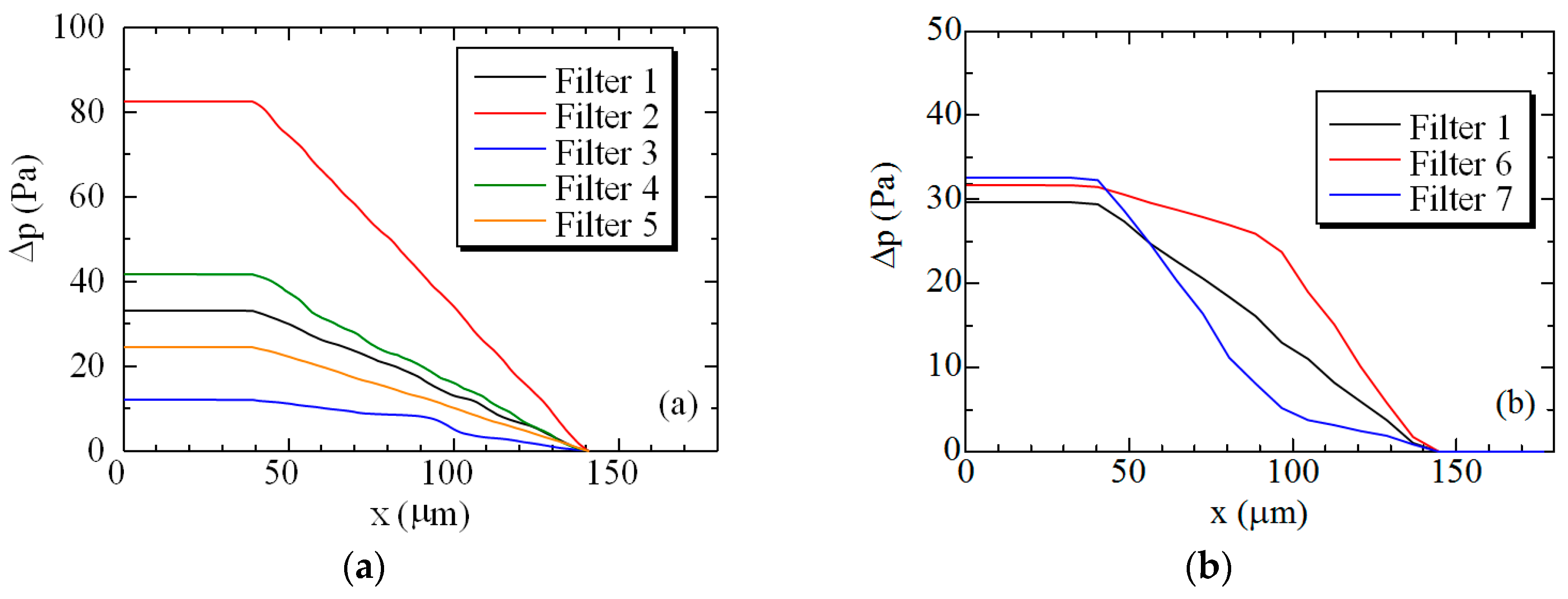
Even in cold flow, a complex flow pattern is observed, with a number of flow paths. If the porous structure is uniform, the linear pressure drops along the flow direction is observed across the filter wall. As the porosity is lower, or pore size is smaller, the initial pressure drop increases. In the case of non-uniform filters, the gradient of the pressure drop changes, but simply, the initial pressure drop is almost the same if the averaged porosity and pore size are the same.

(2)

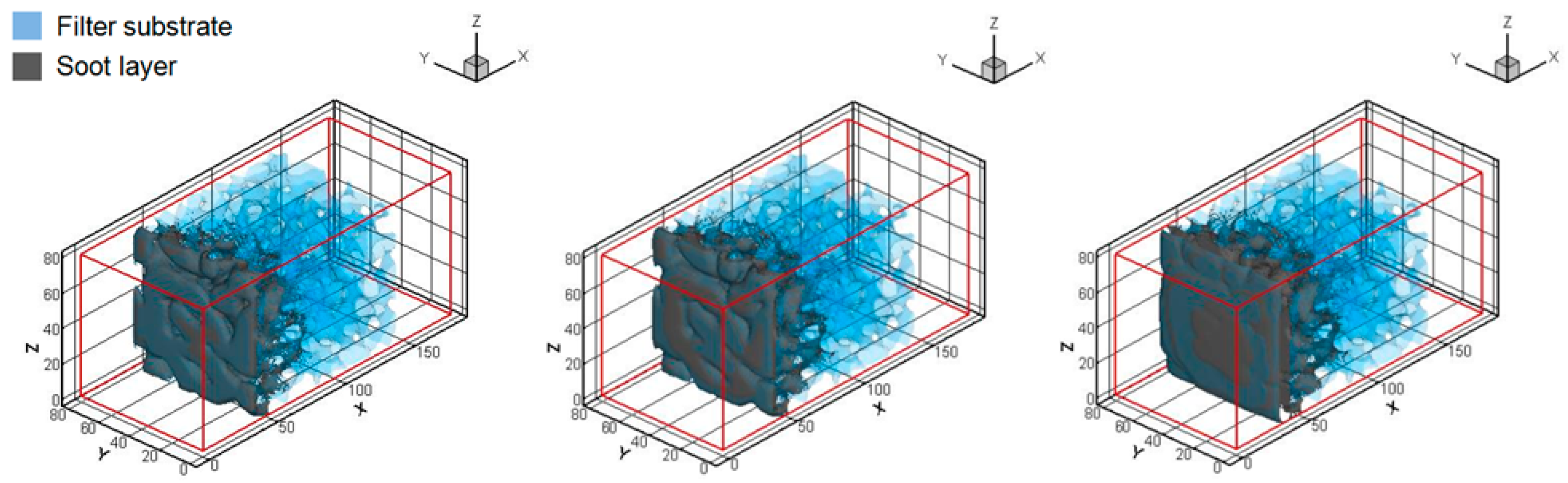
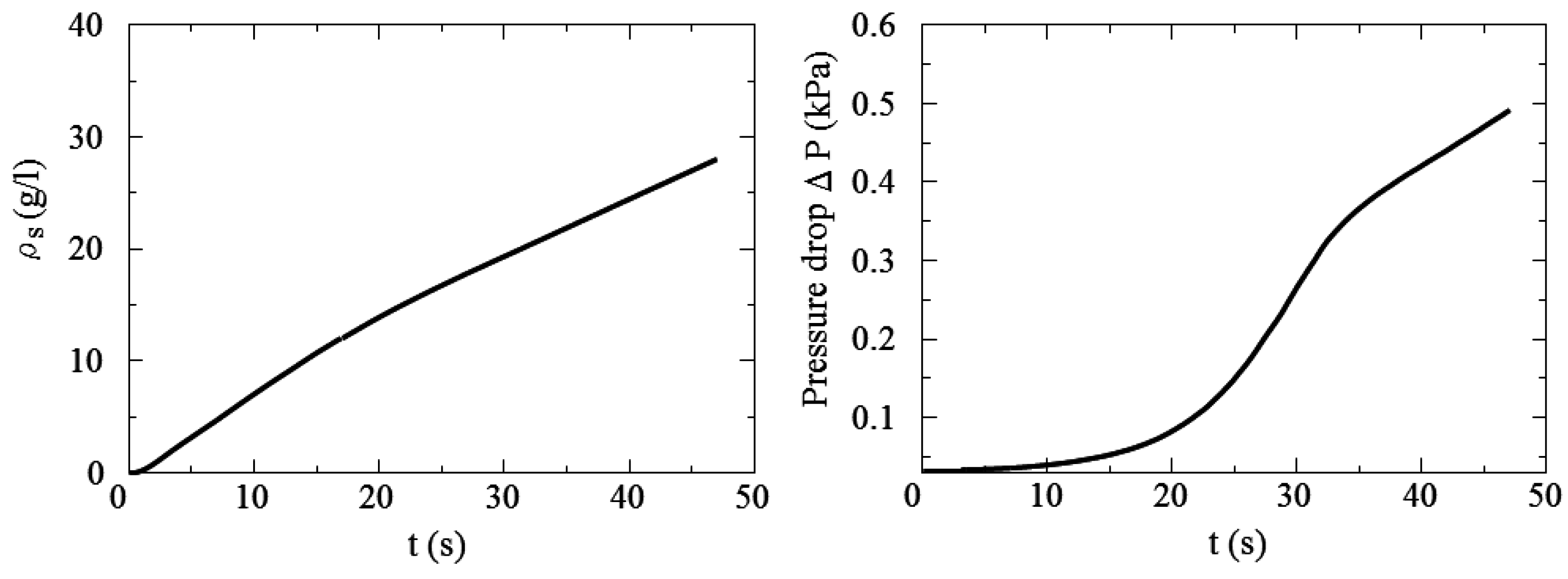
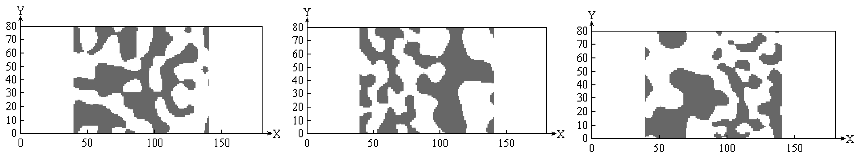
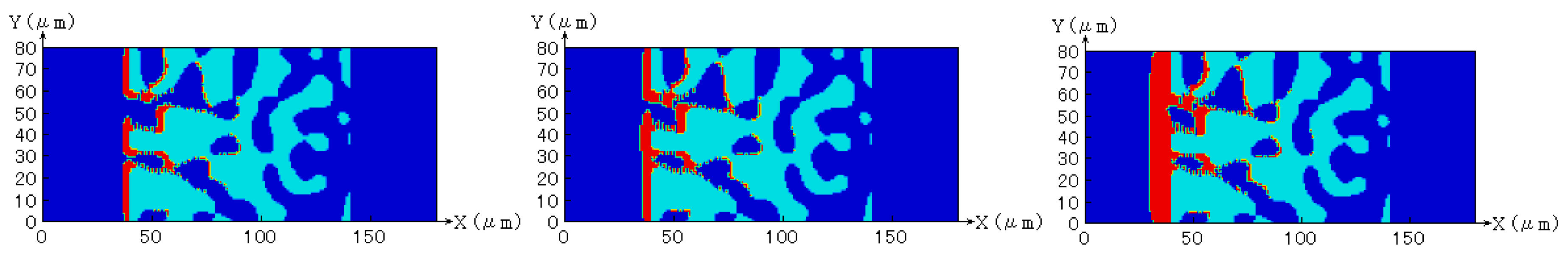
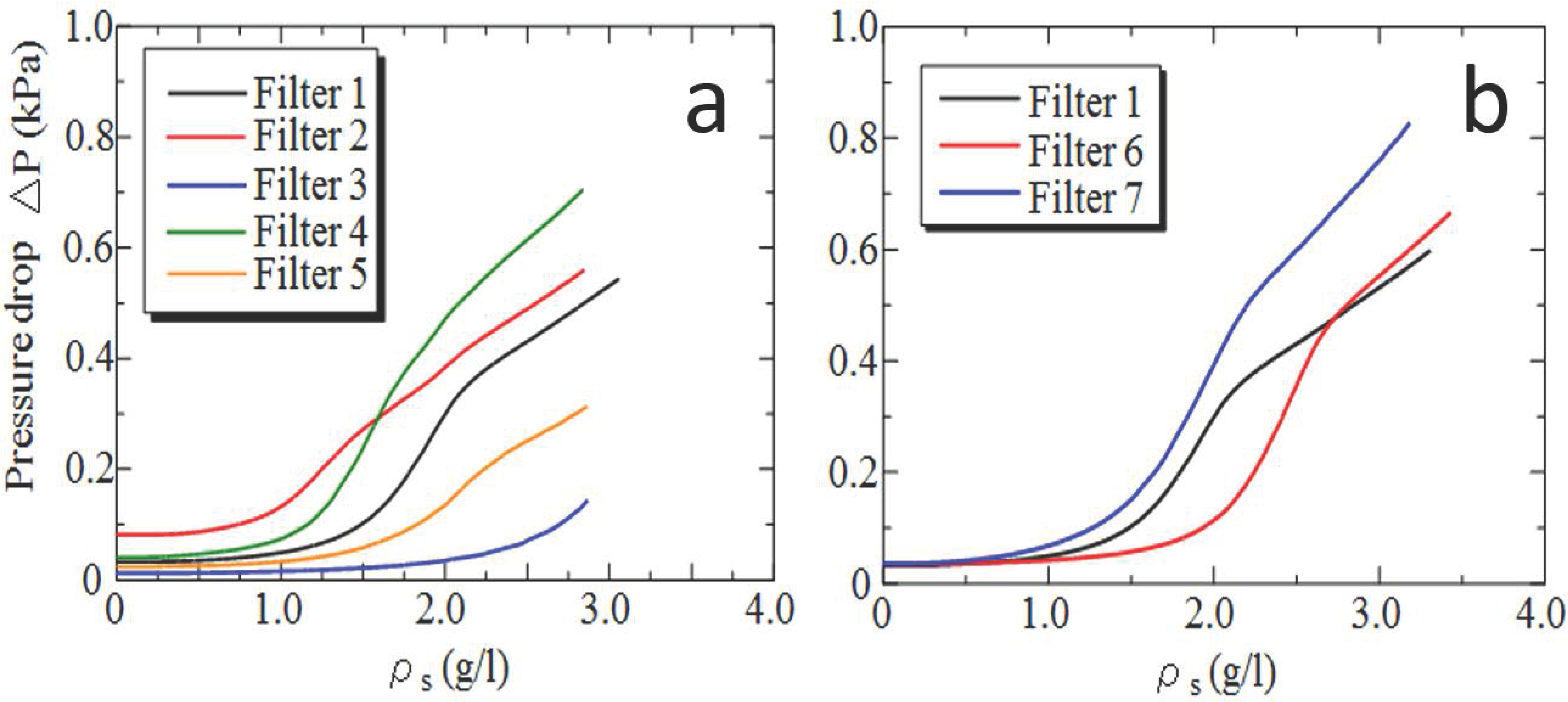
When the flow path inside the filter is plugged with soot, the filter backpressure increases. Gradually, pores at the filter surface are clogged with soot, forming a soot deposition layer on the filter wall surface (called a soot cake). Once, the soot cake is formed, all the soot is trapped by this soot layer. Then, a transition between depth filtration and surface filtration is observed. By comparing the pressure drop of seven filters, Filter 5 with high porosity could be appropriate, because the pressure rise during the depth filtration is suppressed.

References

1. Clerc, J.C. Catalytic Diesel Exhaust After-Treatment. Appl. Catal. B-Environ. 1996, 10, 99–115. [Google Scholar] [CrossRef]
2. Johnson, T.V. Diesel emissions in review. SAE Int. J. Engines 2011, 4, 143–157. [Google Scholar] [CrossRef]
3. Kittelson, D.B. Engines and nanoparticles: A review. J. Aerosol Sci. 1998, 29, 575–588. [Google Scholar] [CrossRef]
4. Stratakis, G.A.; Psarianos, D.L.; Stamatelos, A.M. Experimental investigation of the pressure drop in porous ceramic diesel particulate filters. Proc. Inst. Mech. Eng. D-J. Automob. Eng. 2002, 216, 773–784. [Google Scholar] [CrossRef]
5. Wirojsakunchai, E.; Schroeder, E.; Kolodziej, C.; Foster, D.E.; Schmidt, N.; Root, T.; Kawai, T.; Suga, T.; Nevius, T.; Kusaka, T. Detailed diesel exhaust particulate characterization and real-time DPF filtration efficiency measurements during PM filling process. SAE Tech. Pap. 2007, 2007, 1–14. [Google Scholar]
6. Tsuneyoshi, K.; Takagi, O.; Yamamoto, K. Effects of washcoat on initial PM filtration efficiency and pressure drop in SiC DPF. SAE Tech. Pap. 2011, 2011, 1–10. [Google Scholar]
7. Yamamoto, K.; Takada, N.; Misawa, M. Combustion simulation with lattice Boltzmann method in a three-dimensional porous structure. Proc. Comb. Inst. 2005, 30, 1509–1515. [Google Scholar] [CrossRef]
8. Yamamoto, K.; Ohori, S. Simulation on flow and soot deposition in diesel particulate filter. Int. J. Eng. Res. 2013, 14, 333–340. [Google Scholar] [CrossRef]
9. Yamamoto, K.; Satake, S.; Yamashita, H.; Takada, N.; Misawa, M. Fluid simulation and X-ray CT images for soot deposition in a diesel filter. Eur. Phys. J. 2009, 171, 205–212. [Google Scholar] [CrossRef]
10. Yamamoto, K.; Nakamura, M.; Yane, H.; Yamashita, H. Simulation on catalytic reaction in diesel particulate filter. Catal. Today 2010, 153, 118–124. [Google Scholar] [CrossRef]
11. Yamamoto, K.; Yamauchi, K.; Takada, N.; Misawa, M.; Furutani, H.; Shinozaki, O. Lattice Boltzmann simulation on continuously regenerating diesel filter. Philos. Trans. A 2011, 369, 2584–2591. [Google Scholar] [CrossRef] [PubMed]
12. Atanasov, A.; Uekermann, B.; Pachajoa Mejía, C.A.; Bungartz, H.J.; Neumann, P. Steady-state Anderson accelerated coupling of lattice Boltzmann and Navier–Stokes solvers. Computation 2016, 4, 38–56. [Google Scholar] [CrossRef]
13. Chen, S.; Doolen, G.D. Lattice Boltzmann method for fluid flows. Annu. Rev. Fluid Mech. 1998, 30, 329–364. [Google Scholar] [CrossRef]
14. Succi, S.; Foti, E.; Higuera, F. Three-dimensional flows in complex geometries with the lattice Boltzmann method. Europhys. Lett. 1989, 10, 433–438. [Google Scholar] [CrossRef]
15. Cancelliere, A.; Chang, C.; Foti, E.; Rothman, D.H.; Succi, S. The permeability of a random medium: Comparison of simulation with theory. Phys. Fluids A 1990, 2, 2085–2088. [Google Scholar] [CrossRef]
16. Inamuro, T.; Yoshino, M.; Ogino, F. Lattice Boltzmann simulation of flows in a three-dimensional porous structure. Int. J. Numer. Methods Fluids 1999, 29, 737–748. [Google Scholar] [CrossRef]
17. Bernsdorf, J.; Brenner, G.; Durst, F. Numerical analysis of the pressure drop in porous media flow with lattice Boltzmann (BGK) automata. Comput. Phys. Commun. 2000, 129, 247–255. [Google Scholar] [CrossRef]
18. Yoshino, M.; Inamuro, T. Lattice Boltzmann simulations for flow and heat/mass transfer problems in a three-dimensional porous structure. Int. J. Numer. Methods Fluids 2003, 43, 183–198. [Google Scholar] [CrossRef]
19. Abdallaoui, M.E.; Hasnaoui, M.; Amahmid, A. Numerical simulation of natural convection between a decentered triangular heating cylinder and a square outer cylinder filled with a pure fluid or a nanofluid using the lattice Boltzmann method. Powder Technol. 2015, 277, 193–205. [Google Scholar] [CrossRef]
20. Yamamoto, K.; Satake, S.; Yamashita, H.; Takada, N.; Misawa, M. Lattice Boltzmann simulation on porous structure and soot accumulation. Math. Comput. Simul. 2006, 72, 257–263. [Google Scholar] [CrossRef]
21. Yamamoto, K.; Takada, N. LB simulation on soot combustion in porous media. Phys. A 2006, 362, 111–117. [Google Scholar] [CrossRef]
22. Yamamoto, K.; Satake, S.; Yamashita, H. Microstructure and particle-laden flow in diesel particulate filter. Int. J. Ther. Sci. 2009, 48, 303–307. [Google Scholar] [CrossRef]
23. Qian, Y.H.; D’Humières, D.; Lallemand, P. Lattice BGK models for Navier-Stokes equation. Europys. Lett. 1992, 17, 479–484. [Google Scholar] [CrossRef]
24. Muntean, G.G.; Reactor, D.; Herling, D.; Lessor, D.; Khaleel, M. Lattice-Boltzmann diesel particulate filter sub-grid modelling – a progress report. SAE Tech. Pap. 2003, 2003, 1–8. [Google Scholar]
25. Hayashi, H. Lattice Boltzmann method and its application to flow analysis in porous media. R D Rev. Toyota CRDL 2003, 38, 17–25. [Google Scholar]
26. Dillon, H.; Stewart, M.; Maupin, G.; Gallant, T.; Li, C.; Mao, F.; Pyzik, A.; Ramanathan, R. Optimizing the advanced ceramic material for diesel particulate filter applications. SAE Tech. Pap. 2007, 2007, 1–8. [Google Scholar]
27. Konstandopoulos, A.G.; Skaperdas, E. Microstructural properties of soot deposits in diesel particulate traps. SAE Tech. Pap. 2002, 2002, 1–11. [Google Scholar]
28. Hinds, W.C. Aerosol Technology, 2nd ed.; John Wiley & Sons: New York, NY, USA, 1999; pp. 233–259. [Google Scholar]
29. Yamamoto, K.; Yamauchi, K. Numerical simulation of continuously regenerating diesel particulate filter. Proc. Combus. Inst. 2013, 34, 3083–3090. [Google Scholar] [CrossRef]
30. Yamamoto, K.; He, X.; Doolen, G.D. Simulation of combustion field with lattice Boltzmann method. J. Stat. Phys. 2002, 107, 367–383. [Google Scholar] [CrossRef]
31. Zou, Q.; He, X. On pressure and velocity boundary conditions for the lattice Boltzmann BGK model. Phys. Fluids 1997, 9, 1591–1598. [Google Scholar] [CrossRef]
Figure 1. Soot deposition model. (a) Time step of IT1; (b) Time step of IT2; (c) Time step of IT2 + 1.
Computation 04 00046 g001
Figure 2. Calculation domain, showing the inner substrate structure of Filter 6.
Computation 04 00046 g002
Figure 3. Slice images of Filter 1 (left); Filter 6 (middle); and Filter 7 (right).
Computation 04 00046 g003
Figure 4. Flow field with streamline inside DPF, together with porous filter substrate.
Computation 04 00046 g004
Figure 5. Distribution of velocity in (a) x-y plane, (b) x-z plane, (c) y-z plane.
Computation 04 00046 g005
Figure 6. Distribution of pressure averaged in y-z plane; (a) Filters 1 to 5; (b) Filters 1, 6, 7.
Computation 04 00046 g006
Figure 7. Three-dimensional distribution of soot mass fraction in gas phase in Filter 1 at t = 15 s.
Computation 04 00046 g007
Figure 8. Three-dimensional soot layer at t = 15 s (left); 20 s (middle); 35 s (right) in case of Filter 1.
Computation 04 00046 g008
Figure 9. Slice image of soot layer in x-y plane at t = 15 s (left), 20 s (middle), 35 s (right) in case of Filter 1.
Computation 04 00046 g009
Figure 10. Time-variation of deposited soot mass (left) and pressure drop (right) in Filter 1.
Computation 04 00046 g010
Figure 11. Relationship between deposited soot mass and pressure drop in Filters 1 to 7. (a) Filters 1–5; (b) Filters 1, 6, 7.
Computation 04 00046 g011