Abstract
Optimization methods are increasingly used to solve problems in aeronautical engineering. Typically, optimization methods are utilized in the design of an aircraft airframe or its structure. The presented study is focused on improvement of aircraft flight control procedures through numerical optimization. The optimization problems concern selected phases of flight of a light gyroplane—a rotorcraft using an unpowered rotor in autorotation to develop lift and an engine-powered propeller to provide thrust. An original methodology of computational simulation of rotorcraft flight was developed and implemented. In this approach the aircraft motion equations are solved step-by-step, simultaneously with the solution of the Unsteady Reynolds-Averaged Navier–Stokes equations, which is conducted to assess aerodynamic forces acting on the aircraft. As a numerical optimization method, the BFGS (Broyden–Fletcher–Goldfarb–Shanno) algorithm was adapted. The developed methodology was applied to optimize the flight control procedures in selected stages of gyroplane flight in direct proximity to the ground, where proper control of the aircraft is critical to ensure flight safety and performance. The results of conducted computational optimizations proved the qualitative correctness of the developed methodology. The research results can be helpful in the design of easy-to-control gyroplanes and also in the training of pilots for this type of rotorcraft.
1. Introduction
Optimization methods are widely considered to be very effective tools that can significantly improve the performance of contemporarily designed and constructed aircraft. Typically, optimization methods are utilized in the design of an aircraft airframe or its structure that may be optimized simultaneously using a multi-disciplinary approach [1,2,3]. Fast development of both computational methods and computer hardware offers opportunities to expand the range of applications of optimization methods. As part of this trend, the application of modern computational methods to optimize aircraft flight control procedures is presented in this paper. The developed methodology for the optimization of flight control procedures is discussed in an example of the flight of a light gyroplane.
A gyroplane is an aerodyne equipped with unpowered main rotor and engine-powered propeller, generating a thrust force necessary to move the aircraft forward. During gyroplane flight, the air flowing around the rotating blades of the main rotor generates an aerodynamic reaction whose vertical component balances the aircraft weight, while the aerodynamic moment is driving the main rotor that rotates in autorotation. However, to induce the autorotation phenomenon, the rotor should be initially pre-rotated, which is usually done by the engine driving the propeller. Before the gyroplane loses contact with the ground, the drive of the rotor must be disconnected because this type of rotorcraft does not have any anti-torque devices.
The primary flight control means of gyroplanes are:
- longitudinal and lateral tilting of the rotor shaft to ensure a pitch and roll control;
- deflections of the rudder to ensure a yaw control.
Gyroplanes may be optionally equipped with the following secondary flight controls:
- a pre-rotator that drives the rotor to initiate its rotation,
- a changeable collective pitch of rotor blades that may be used for torque reduction in pre-rotation and is necessary to conduct so-called “jump takeoff.”
The regular takeoff of a gyroplane is similar to the typical takeoff of an airplane. The gyroplane, with pre-rotated main rotor, starts accelerating along the runway. The rotor generates more and more lift (thrust). When the lift exceeds the weight of the aircraft, the gyroplane takes off. Gyroplanes usually need a short runway to conduct regular takeoff and mostly belong to the STOL (Short Takeoff and Landing) category of aircraft.
In the case of so-called “jump takeoff”, the gyroplane takes off directly from the ground, without a run along the runway. To perform this maneuver, the rotor head design should allow for changing the angle of blade collective pitch during the flight. After initial pre-rotation of the rotor, the drive is disconnected and simultaneously the higher angle of the blade collective pitch is established. The inertia-driven rotor generates high thrust, which makes the gyroplane jump upwards. The propeller starts driving the gyroplane in the horizontal direction, which makes the horizontal velocity grow; after some time the rotor starts rotating in autorotation, similar to the case of the regular takeoff.
All studies presented in this paper have been conducted for the gyroplane presented in Figure 1. The gyroplane is equipped with a teetering main rotor, three-bladed tractor-type propeller, front landing gear, and inverted V-tail that also serves as a rear landing gear. Like most gyroplanes, the main rotor of the presented gyroplane is a simple design. It is a two-bladed, teetering rotor. Its blades have a rectangular planform, uniform spanwise distribution of airfoil, and are not twisted. To enhance the controllability of the gyroplane, its rotor-head design enables control of the collective pitch of rotor blades.
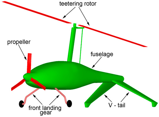
Figure 1.
Gyroplane model used as the basis for analyses in this paper.
An effective and safe takeoff of the gyroplane requires accurate and rapid deflections of flight control devices. This is especially true for the control of the rotor pitch angle, which has to be changed optimally during the takeoff so as to enhance the autorotation effect as much as possible. Additionally, during jump takeoff, the dynamic changes of the rotor pitch angle have to be synchronized with the dynamic changes of the collective pitch of the rotor blades.
The main idea of the presented research was to search for optimal procedures to control the gyroplane flight through the application of a numerical optimization methodology. To realize this idea, the following three main goals of the research undertaken were established:
- To develop a computational methodology for the simulation of gyroplane flight, especially directed towards high-fidelity simulations of takeoff and ascent.
- To develop a numerical optimization methodology that would be applicable to solving problems concerning the optimization of rotorcraft flight control procedures.
- To optimize flight control procedures (i.e., functions describing time-varying settings of the flight control devices) during the classic takeoff and jump takeoff of the gyroplane, so as to achieve measurable improvement in the aircraft performance of these flight modes.
Numerical optimization methods are widely utilized in rotorcraft engineering. Most of them are directed towards optimization of the rotorcraft crucial components such as main rotors or tail rotors. Nowadays, such optimization problems are usually formulated in multidisciplinary form [4]. This includes more and more reliable methods in such areas as Computational Fluid Dynamics (CFD), Computational Structural Mechanics (CSM) or Flight Dynamics. On the other hand, attempts are made to automate the design process itself, by applying numerical optimization methods. The CFD methods have reached sufficient maturity to compute very accurately helicopter rotor aerodynamic performance. The current CFD codes’ efficiency potentially enables their use in automatic optimization chains. Such optimization strategies involving URANS (Unsteady Reynolds-Averaged Navier–Stokes) solvers have been applied in aeronautics on fixed wing configurations [5,6] or via adjoint formulation on aircraft configurations [7,8] and have demonstrated their ability to be successfully and efficiently integrated in design cycles. Alternative approaches are based on stochastic optimization methods (e.g., Genetic Algorithm). Among others, such an approach was applied in [3] for optimization of helicopter fuselage (with simulation of main and tail rotor influence) as well as in [1,2] for multidisciplinary optimization of aircraft wings. To cope with the extreme complexity of coupling advanced methods of CFD and numerical optimization, some authors utilize surrogate models of physical phenomena, as presented in [9,10]. In [11] the authors describe an optimization strategy for helicopter rotor blade shape, based on the coupling of an optimization gradient method with a 3D Navier–Stokes solver.
Advanced numerical optimization methods coupled with Navier–Stokes solvers are actually used mostly for optimization of aircraft external shapes (aerodynamic design) or structure. In the case of optimization of rotorcraft flight control procedures, simplified computational models of aerodynamics are usually used. In particular, this concerns advanced computational tools dedicated for flight control optimization. Such tools usually utilize simple models of rotorcraft aerodynamics. The aerodynamic effects generated by crucial components of a rotorcraft, such as the main rotor or tail rotor, are usually modeled using the lifting-line theory or are even based on databases of global aerodynamic characteristics of these rotors. For the case of the rotorcraft flight control design and optimization tool CONDUIT, details regarding the optimization methods and aerodynamic models are discussed thoroughly in [12,13].
In comparison to previously used computational tools supporting the design and optimization of rotorcraft flight control, the approach discussed in this paper is not directly geared to industrial applicability but rather to exploring new solutions that could in future be applied to designing flight control systems. The proposed solution distinguishes itself from most of the currently utilized approaches by the following assumptions:
- The rotorcraft flight control optimization is based on advanced, gradient-based optimization methods coupled with advanced CFD methods used directly during the rotorcraft flight simulation for the current determination of aerodynamic loads acting on the aircraft.
- The developed methodology is applied to optimize the gyroplane flight control procedures (while most of the applications cited in the literature are focused on the optimization of helicopter flight control).
The research presented in the paper is aimed mainly at proving a possibility of successfully using advanced CFD models even in such complex computational problems as the optimization of aircraft flight control procedures, during highly unsteady flight conditions. So far, such an approach has been limited by the computational efficiency of computer systems. However, it is expected that the use of high-fidelity CFD methods can significantly improve the accuracy and reliability of the optimization results. Methods using simplified aerodynamic models are burdened with large errors, especially in relation to the modeling of physical phenomena that play a large role during the takeoff and ascent of the gyroplane. These are, among others, the ground effect (increase of lift in direct proximity of the ground); autorotation; aerodynamic interactions between the main rotor, propeller, fuselage and tail; and the unsteadiness of all physical phenomena. Advanced CFD models enable taking into account such phenomena; therefore, their application should significantly improve the accuracy of modeling of gyroplane takeoff and ascent.
2. Research Methodology
The general scheme of the developed methodology of rotorcraft flight simulation is presented in Figure 2. The flight simulation procedure is embedded in the URANS (Unsteady Reynolds Averaged Navier–Stokes) solver ANSYS FLUENT [14]. Flow effects caused by rotating lifting surfaces are modeled by application of the developed UDF (User Defined Function) module Virtual Blade Model (VBM) [3], which is compiled and linked with the essential code of the ANSYS FLUENT software. In the VBM approach, real rotors are replaced by volume discs influencing the flow field in a similar manner to rotating blades. Time-averaged aerodynamic effects of rotating lifting surfaces are modeled by means of artificial momentum source terms placed inside the volume-disc zones placed in regions of activity of real rotors. Such zones, replacing the real rotor and propeller in investigated gyroplane, are shown in Figure 3. The momentum rates, injected from these zones into the fluid, are evaluated based on the Blade Element Theory, associating local flow parameters in rotor-disc zones with aerodynamic characteristics of blade airfoils. Data bases of these characteristics (in general: lift and drag coefficients as functions of angle of attack, for several sets of Mach and Reynolds numbers, similar to those that are expected on the real rotor blades) should be prepared before starting the flight simulation. The original VBM code was significantly modified and expanded by the author of this paper. Beside the essential modules ANSYS FLUENT and VBM, the methodology presented in Figure 2 utilizes two additional modules. The module FLIGHT-DYNAMIC gathers information on all instantaneous loads acting on the rotorcraft and solves six-degrees-of-freedom equations of rigid body motion. The module KINEMATICS is responsible for modeling of effects of motion and changes of rotorcraft geometry, which is realized through a redefinition of the boundary conditions for the ANSYS FLUENT solver and through deformations of computational mesh. The computational model of the gyroplane, shown in Figure 3, was developed so as to enable simulation of flight in proximity to the ground and tilting of the rotor. These motions are realized through appropriate deformations of computational mesh, which is done with the use of the Dynamic Mesh technique, implemented in the ANSYS FLUENT solver. Examples of such deformations of computational mesh are presented in Figure 4. Additionally, the developed model enables deflecting the gyroplane control surfaces (option not used in the presented study), which is realized through application of Sliding-Mesh and Non-Conformal-Interface techniques implemented in ANSYS FLUENT.
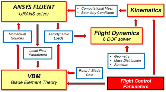
Figure 2.
General scheme of the developed methodology of rotorcraft-flight simulation.
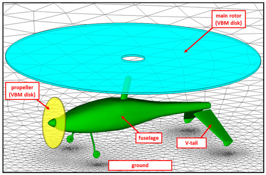
Figure 3.
Computational model of the gyroplane flying in proximity to the ground.
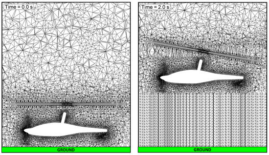
Figure 4.
Cross-section of computational mesh around the gyroplane in two different stages of flight Left: a ground pre-rotation, right: a forward flight a few meters above the ground.
All URANS simulations discussed in this paper were conducted with the one-equation, Spalart–Allmaras turbulence model.
During gyroplane takeoff and ascent simulations, the flight velocity was changing within the range of 0 m/s (at the beginning of takeoff) to approx. 25 m/s. Taking into account the diameter of the main rotor 9.4 m as the reference length, the gyroplane flight Reynolds numbers were changing within the range of 0 to approx. 16 × 106.
The aerodynamic characteristics databases of airfoils of blades of the gyroplane main rotor and propeller, necessary for the VBM module, were calculated using a 2D variant of ANSYS FLUENT software. For the main rotor blade airfoils, the calculations were conducted for Mach number range 0.2 ÷ 0.82 and Reynolds number range 1 × 10⁶ ÷ 5.7 × 10⁶. For the propeller blade airfoils, these ranges were: 0.2 ÷ 0.93 for Mach number and 1 × 10⁶ ÷ 6.5 × 10⁶ for Reynolds number.
The computational mesh was generated and validated using the ANSYS GAMBIT—a commonly used mesh generator included in earlier distributions of ANSYS CFD software packages. During the rotorcraft flight simulations, the mesh was deformed due to: tilting of the main rotor, changeable distance between the aircraft and the ground, and (optional) deflections of control surfaces. This last type of mesh deformation was not conducted in the flight simulations discussed in this paper. The quality of the mesh deformed during the simulations was controlled by both the internal procedures of the ANSYS FLUENT and the dedicated procedures included within the developed in-house UDF module KINEMATICS.
The total number of cells of the computational mesh used in the CFD simulations discussed in this paper was 2,157,487. This number refers to the initial state of the mesh. During the rotorcraft flight simulation, this number could be slightly changed due to remeshing procedures conducted with respect to the mesh surrounding the cylindrical zone modeling the main rotor. The mesh filling the space between the aircraft and the ground was not remeshed, having a constant number of cells during the whole simulation.
During the flight control optimization process, gyroplane flight simulations were conducted simultaneously for several different flight control procedures. On a typical single-processor computer system, realization of a single simulation of gyroplane takeoff and initial stage of ascent, with a time step equal 0.01 s, required approximately 15 h of computational time. In total, the complete single step of the optimization process was conducted within 30 h. Increasing the time step of integration of equations of gyroplane motion could proportionally decrease the total time of computations.
The described complex model of the gyroplane flight was used in optimization studies on flight control procedures during the gyroplane takeoff. Though the developed methodology enables the solution of six-degrees-of-freedom rotorcraft flight dynamics, the simulations presented in the paper were conducted taking into account only force balance equations, while moment balance equations were omitted. To reduce the computational complexity of the optimization problem, it was assumed that it would not concern directional stability and control. It was assumed that, during the simulated flight states, the pilot will be able to provide the correct directional position and direction of the rotorcraft flight.
The method of computational simulation of gyroplane flight has been applied in optimization studies on flight control procedures. In these studies, functions describing changes in time of the main gyroplane flight control means (i.e., tilt of the main-rotor shaft and collective pitch of rotor blades) have been parameterized. In general, they were assumed to have the form of continuous, piecewise linear functions, defined in a domain consisting of M sections:
where (t0, t1, …, tM) were knots defining the function domain while (f0, f1, …, fM) were function values in subsequent knots. In the presented approach both the function knots {ti}i=0,1,…,M and values {fi}i=0,1,…,M were expressed as linear functions of a few unknown real numbers—the design parameters. In practice, when defining a given optimization problem, small values of M are preferred so as to reduce the number of independent design parameters, and thus the dimension of the problem. On the other hand, in every case the number M was selected so as to ensure sufficient degree of freedom of flight control procedures. The objective function, considered as a function of unknown design parameters, was defined as the altitude that would be achieved by the gyroplane after reaching the assumed distance from the takeoff point.
To solve the defined optimization problem, the appropriately adapted BFGS Algorithm [15] has been applied. The method BFGS, named after C.G. Broyden, R. Fletcher, D. Goldfarb and D. Shanno, belongs to quasi-Newton methods—a class of hill-climbing optimization techniques that seek a stationary point of a given objective function (preferably twice continuously differentiable). Gradient-based methods utilize a necessary condition for optimality, saying that at an optimum point the gradient of the objective function is a zero vector. Usually such methods do not guarantee convergence to an exact optimum, unless the objective function has a quadratic Taylor expansion near an optimum. However, the BFGS Algorithm has proven to have good performance even in cases where the objective functions were not smooth.
In quasi-Newton methods, including the BFGS Algorithm, the Hessian matrix of second derivatives does not need to be evaluated directly. Instead, the Hessian matrix is approximated using updates specified by gradient evaluations or approximate gradient evaluations. The latter approach has been applied in the presented optimization studies.
Like in all cases of gradient-based methods, the optimal solution has been searched for in sequential iterative steps. In each step, the components of the gradient vector (partial derivatives of the objective function with respect to the unknown design parameters) were evaluated by means of a one-sided finite-difference approximation. In the presented approach, this required performing at least N + 1 simulations of the gyroplane flight, where N was the number of design parameters.
In each step of the BFGS algorithm, an auxiliary one-dimensional optimization problem is solved. The problem consists of searching for the optimal movement in the newly determined search direction. In the presented approach, the solution of this problem required conducting several additional simulations of gyroplane flight in each sequential step of the optimization process. It should be mentioned that the BFGS method has also been developed in a variant with simple box constraints [16] and usually this variant has been applied in the presented optimization studies.
3. Optimization of Gyroplane Takeoff Control Procedures
The two examples presented below of numerical optimizations of flight control procedures pertain to two types of takeoff of the gyroplane: classic takeoff and jump takeoff. In both cases, the optimization process aimed at maximization of the altitude reached by the gyroplane after traveling a certain distance from the takeoff place. Both optimizations were conducted for the same general flight conditions:
- total mass of the gyroplane: 600 kg;
- maximum static thrust of the propeller: 2943 N (during takeoff, when the forward velocity of the vehicle was growing, the thrust of the propeller was changing, which was a result of modeling the propeller effects through VBM methodology).
3.1. Classic Takeoff of the Gyroplane
The optimization of classic takeoff control procedure has been conducted with respect to time varying pitch angle of main rotor (ϕR), which was considered the only flight control parameter. The angle of collective pitch of rotor blades (θ0), unchangeable during the flight, has been assumed as an additional unknown parameter. Based on these assumptions, the flight control parameters ϕR(t) and θ0(t) were assumed to have the form defined by Equation (1) as piecewise linear functions ΨM(t). Parameters M, {ti}i=0,1,…,M and {fi}i=0,1,…,M of these functions were related to the design parameters D1, F1 and F2 presented in Figure 5, according to the following dependencies:
ϕR(t) = Ψ2(t), for: t0 = 0, t1 = D1, t2 = +∞, f0 = 0, f1 = F1, f2 = F1
θ0(t) = Ψ1(t), for: t0 = 0, t1 = +∞, f0 = F2, f1 = F2.
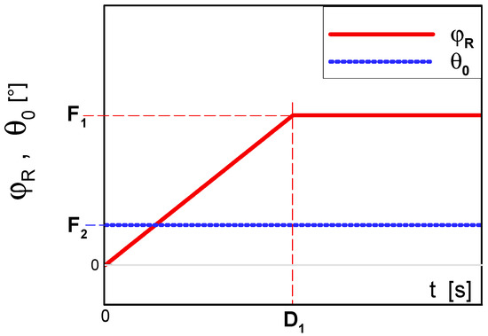
Figure 5.
Parametric model of the gyroplane flight control procedure utilized in the optimization of the classic takeoff of the gyroplane.
Based on the opinions of gyroplane designers and pilots, such a relatively simple parameterization should sufficiently approximate the real flight control procedures utilized during the takeoff and ascent of gyroplane. This especially concerns the presented study, which is more about demonstration than implementation. In the discussed case, the optimization aimed at maximization of the altitude (H) reached by the gyroplane after traveling the distance X = 200 m from the initial position, which is explained in Figure 6. The optimization problem was formulated mathematically as a search for the set of the design parameters D1, F1 and F2 maximizing the following objective function Φ:
taking into account the following constraints:
where λ1—limit of angular speed of change of ϕR, ϕRmax—maximum of rotor pitch and θ0max—maximum of blade collective pitch.
Φ(D1, F1, F2) = H(X = 200 m),
D1 > 1,
F2 ≤ θ0max,
| F1/D1 | ≤ λ1,
F1 ≤ ϕRmax,
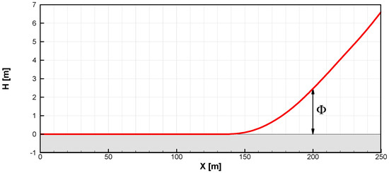
Figure 6.
Definition of the objective (Φ) for the optimization of classic takeoff control strategy.
The optimization problem has been solved iteratively using the BFGS algorithm, discussed in Section 2. In the sequential steps of the optimization process, this procedure has been improved from the point of view of maximizing the objective function Φ in Equation (4). In each iterative step, the partial derivatives of the objective function Φ with respect to the unknown design parameters had to be approximated due to the requirements of the BFGS Algorithm. These derivatives were evaluated by means of the one-sided finite-difference approximation. This required performing at least N + 1 simulations of the classic takeoff of the gyroplane, where N = 3 was the number of independent variables in Equation (4). In addition, solving the auxiliary one-dimensional problem of finding the optimal movement in the newfound search direction, eight additional classic gyroplane takeoff simulations were conducted in each optimization step.
In the presented optimization process only four iterative steps of the BFGS method have been conducted. Due to time limits, the calculations were not continued until full convergence of the BFGS algorithm was achieved. Changes in the objective function Φ in the four sequential steps are shown in Figure 7. The presented results show that at a distance of 200 m, the gyroplane controlled by the optimized procedure reached an altitude about 5 m higher than the baseline. The improved final flight control procedure is compared with the baseline procedure in Figure 8.
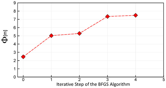
Figure 7.
Values of the maximized objective Φ in sequential iterative steps of the process of optimization of the classic takeoff control procedure of the gyroplane.
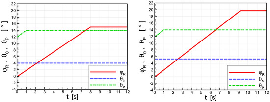
Figure 8.
Comparison of the baseline (left) and optimized (right) classic takeoff control procedures, showing the pitch angle of main rotor (ϕR), collective pitch of rotor blades (θ0) and collective pitch of propeller blades (θP) as functions of time (t).
The final solution of the optimization over the baseline procedure differs in the blade collective pitch greater by 1.3°, the rotor pitch angle greater by 4.7° and angular speed of change of rotor pitch greater by 14.3%. Figure 9 compares gyroplane flight trajectories during the classic takeoff for two gyroplane flight control strategies: baseline and optimized. Compared to the baseline, the aircraft trajectory corresponding to the optimized procedure shows a shorter run of the aircraft on the runway and faster climb, at least during arrival to the assumed altitude-control point, localized 200 m from the starting point. As shown in Figure 10, during the classic takeoff and initial stage of ascent, the flight velocity (V) of the gyroplane controlled by the optimized procedure was lower (by approx. 3 m/s) than the velocity of gyroplane controlled by baseline procedure.
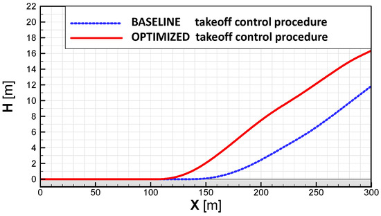
Figure 9.
Aircraft trajectories obtained for the baseline and optimized procedures of flight control during the classic takeoff of the gyroplane.
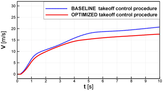
Figure 10.
Aircraft flight velocity (V) vs. time (t) during the classic takeoff, for the baseline and optimized procedures of gyroplane flight control.
Figure 11, Figure 12 and Figure 13 present snapshots of velocity magnitude contours around the gyroplane, taken during the classic takeoff simulation at t = 0, 10, 17.5 s (time elapsed from the beginning of run on a runway), for two compared flight control strategies: baseline and optimized.
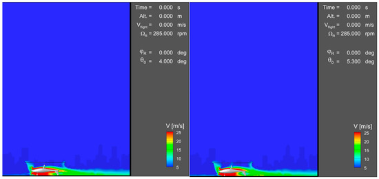
Figure 11.
Comparison of velocity magnitude contours around the gyroplane during the classic takeoff, for two configurations related to baseline (left) and optimized (right) flight control procedures. The initial time (t = 0 s) of the aircraft run on a runway.
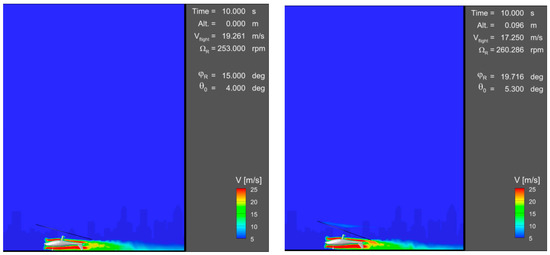
Figure 12.
Comparison of velocity magnitude contours around the gyroplane during the classic takeoff, for two configurations related to baseline (left) and optimized (right) flight control procedures. Time elapsed from the beginning of the aircraft run: t = 10 s.
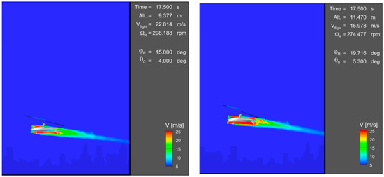
Figure 13.
Comparison of velocity-magnitude contours around the gyroplane during the classic takeoff, for two configurations related to baseline (left) and optimized (right) flight control procedures. Time elapsed from the beginning of the aircraft run: t = 17.5 s.
3.2. Jump Takeoff of the Gyroplane
Improvement of gyroplane flight control strategy during the jump takeoff was conducted based on the numerical optimization approach described in Section 2. In this case, the optimization was conducted with respect to the time-varying pitch angle of the main rotor (ϕR) and the angle of collective pitch of the rotor blades (θ0). Based on these assumptions, the time-varying flight control parameters ϕR(t) and θ0(t) were assumed to have the form defined by Equation (1) as piecewise linear functions ΨM(t). Parameters M, {ti}i=0,1,…,M and {fi}i=0,1,…,M of these functions were related with the presented in Figure 14 design parameters D1, D2, D3, D4, F1, F2 and F3 according to the following dependencies:
ϕR(t) = Ψ3(t), for: t0 = 0, t1 = D1, t2 = D1 + D2 , t3 = +∞, f0 = 0, f1 = 0, f2 = F1, f3 = F1
θ0(t) = Ψ4(t), for: t0 = 0, t1 = 1, t2 = 1 + D3, t3 = 1 + D3 + D4, t4 = +∞, f0 = 0, f1 = F2, f2 = F2, f3 = F3, f4 = F3.
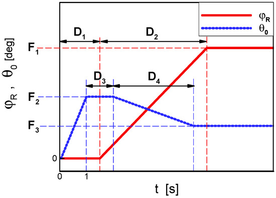
Figure 14.
Parametric model of the gyroplane flight control procedure utilized in the optimization of jump takeoff of the gyroplane.
Based on the opinions of gyroplane designers and pilots, such a relatively simple parameterization should sufficiently approximate the real flight control procedures utilized during the takeoff and ascent of gyroplane. This especially concerns the presented research, which is more about demonstration than implementation. In the discussed case, the optimization aimed at maximization of the altitude (H) reached by the gyroplane after traveling the distance X = 100 m from the initial position, which is explained in Figure 15. The optimization problem was formulated mathematically as a search for values of the design parameters D1, D2, D3, D4, F1, F2 and F3 maximizing the following objective function Φ:
taking into account the following constraints:
where λ1, λ2—limits of angular speed of changes of ϕR and θ0 respectively, ϕRmax—maximum of rotor pitch and θ0max maximum of blade collective pitch. The defined optimization problem has been solved by application of the BFGS algorithm. At every step of the iterative process of the optimization, the gradient of the objective function Equation (11) was determined using the one-sided finite-difference approximation. This required conducting at least N + 1 (where N = 7) independent simulations of gyroplane jump takeoff for different sets of values of unknown design parameters D1, D2, D3, D4, F1, F2, and F3. In addition, to solve the auxiliary one-dimensional problem of finding the optimal movement in the newfound search direction, eight additional gyroplane jump takeoff simulations were performed at each optimization step.
Φ(D1, D2, D3, D4, F1, F2, F3) = H(X = 100 m),
D1 ≥ 0, D2 ≥ 1, D3 ≥ 0, D4 ≥ 1,
F2 ≤ θ0max,
| F1/D2 | ≤ λ1,
| (F2 − F3)/D4 | ≤ λ2,
F1 ≤ ϕRmax,
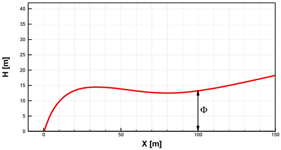
Figure 15.
Definition of the objective (Φ) for the optimization of jump takeoff control strategy on the example of a gyroplane trajectory controlled by the baseline procedure.
The optimization process consisted in gradual improvement of this strategy, so as to increase as much as possible the product of Equation (6). In the present optimization only four iterative steps of the BFGS method have been conducted. Due to time limits, the calculations have not been continued until full convergence of the BFGS algorithm was achieved. Changes in the objective function Φ (Equation (6)) in the sequential steps are presented in Figure 16. The final solution of the optimization is compared with the baseline in Figure 17. The presented results show that the optimized flight control strategy is characterized by nearly the same values of parameters F2 and F3. This means that these two parameters might be replaced by only one in the assumed parametric model of flight control strategy (shown in Figure 14) and the phase of decreasing of the rotor pitch, which we assume might be omitted in this model. Figure 18 compares gyroplane flight trajectories during the jump takeoff for two flight control strategies: baseline and optimized. It may be concluded that the optimized trajectory is growing monotonically while the baseline trajectory has a local minimum. Additionally, for the optimized flight control strategy the result of Equation (11) is higher by approximately 5 m than for the baseline strategy. As shown in Figure 19, during the jump takeoff and initial stage of ascent, the flight velocity (V) of the gyroplane controlled by optimized procedure, after 8 s the flight stabilized itself at a level of approx. 17 m/s. In this case, to increase the flight velocity, after the jump takeoff and ascent the backward pitch of the rotor should be reduced. For the baseline flight control procedure, the flight velocity was still growing and it reached V ≈ 25 m/s at t = 25 s. Figure 20, Figure 21 and Figure 22 present snapshots of flow field (velocity magnitude contours) around the gyroplane taken during the jump takeoff at t = 0.5, 1.5, 10 s (time elapsed from the beginning of the takeoff), for two compared flight control strategies: baseline and optimized.
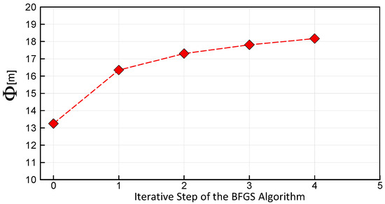
Figure 16.
Values of the maximized objective Φ in sequential iterative steps of the process of optimization of the jump takeoff control procedure of the gyroplane.
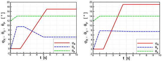
Figure 17.
Comparison of the baseline (left) and optimized (right) jump takeoff control procedures, showing the pitch angle of main rotor (ϕR), collective pitch of rotor blades (θ0) and collective pitch of propeller blades (θP) as functions of time (t).
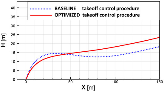
Figure 18.
Aircraft trajectories obtained for the baseline and optimized procedures of flight control during the jump takeoff of the gyroplane.
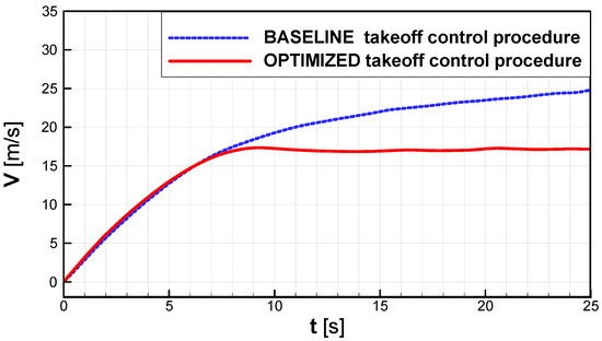
Figure 19.
Aircraft flight velocity (V) vs. time (t) during the jump takeoff, for the baseline and optimized procedures of gyroplane flight control.
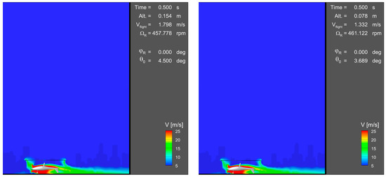
Figure 20.
Comparison of velocity magnitude contours around the gyroplane during the jump takeoff, for two configurations related to baseline (left) and optimized (right) flight control procedures. The initial time moment (t = 0.5 s) of the jump takeoff.
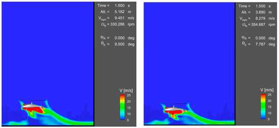
Figure 21.
Comparison of velocity magnitude contours around the gyroplane during the jump takeoff, for two configurations related to baseline (left) and optimized (right) flight control procedures. Time elapsed from the beginning of the jump takeoff: t = 1.5 s.
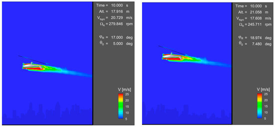
Figure 22.
Comparison of velocity magnitude contours around the gyroplane during the jump takeoff, for two configurations related to baseline (left) and optimized (right) flight control procedures. Time elapsed from the beginning of the jump takeoff: t = 10 s.
4. Discussion
A methodology of computational simulation of gyroplane flight has been developed. The methodology was applied to simulate the classic takeoff of a gyroplane and the so-called “jump takeoff”—a maneuver in which the gyroplane takes off similarly to a helicopter, without the accelerating run along a runway. For these two specific flight conditions, a numerical optimization of flight control procedures has been conducted, using a gradient-based method, the BFGS algorithm. In this process, the assumed design parameters described the time-varying settings of gyroplane flight control: tilt of main-rotor shaft and collective pitch of rotor blades. The optimization aimed at a determination of the flight control procedures that are optimal from the point of view of the highest possible altitude reached by the gyroplane at an assumed distance during both classic takeoff and jump takeoff.
In both cases of optimization discussed, at the control point the gyroplane controlled according to the optimized strategy reached an altitude approximately 5 m higher than the gyroplane controlled according to a baseline flight control procedure.
The presented computational optimizations have proven the qualitative correctness of the developed methodology. So far the obtained quantitative results have not been validated experimentally. The main reason for this is that the gyroplane that is the subject of the investigation has not yet started its flight tests. In addition, the problem is the difficulty of obtaining accurate measurements for the actual flight parameters. In a wind tunnel, investigations of strongly unsteady flight states such as takeoffs or landings are virtually unfeasible. On the other hand, it is difficult to measure a number of important parameters in real test flights. Therefore, a thorough verification of the presented methodology is not possible. However, both the classic and jump takeoffs of other gyroplanes, documented especially in video materials, indicate good convergence, both qualitative and quantitative, with the results of the research presented in this paper. This especially concerns such gyroplane flight parameters as runway run length, flight velocity, flight altitude, duration of takeoff, or shape of trajectory. More accurate comparison of such data concerning takeoffs of other gyroplanes and cases discussed in this paper is impossible because we would need to conduct thorough experimental studies on the gyroplane considered. The gyroplane flight parameters are strongly influenced by such factors as aircraft weight, total area of rotor blades, rotor aerodynamic properties, moments of inertia of rotor and its blades, engine power, performance characteristics of propeller, aerodynamic properties of fuselage, etc. All these data were taken into account in the simulations presented in this paper. Unfortunately, most of these data are not available in the case of potential reference gyroplanes.
It is expected that in the case of alternative definitions of the optimization problem (i.e., another selection of design parameters or another definition of the objective function), the optimization methodology developed would also confirm its effectiveness and reliability.
The research results can be helpful in designing easy-to-control gyroplanes and also in training pilots for this type of rotorcraft. However, the presented methodology seems to have a much wider potential for future applications. These possible applications may concern not only other gyroplanes or rotorcrafts in general but also the optimization of flight control procedures for any aircraft, e.g., taking off or landing airplanes.
Acknowledgments
The research leading to these results was co-financed by the European Regional Development Fund under the Operational Programme Innovative Economy 2007–2013, within the project “Modern Gyroplane Main Rotor”.
Conflicts of Interest
The author declares no conflict of interest.
References
- Rokicki, J.; Stalewski, W.; Zoltak, J. Multi-Disciplinary Optimization of Forward-Swept Wing. In Evolutionary and Deterministic Methods for Design, Optimization and Control with Applications to Industrial and Societal Problems; A Series of Handbooks on Theory and Engineering Applications of Computational; Burczynski, T., Périaux, J., Eds.; International Centre for Numerical Methods in Engineering (CIMNE): Barcelona, Spain, 2011; pp. 253–259. [Google Scholar]
- Stalewski, W.; Zoltak, J. Design of a turbulent wing for small aircraft using multidisciplinary optimization. Arch. Mech. 2014, 66, 185–201. [Google Scholar]
- Stalewski, W.; Zoltak, J. Optimization of the Helicopter Fuselage with Simulation of Main and Tail Rotor Influence. In Proceedings of the 28th ICAS Congress of the International Council of the Aeronautical Sciences, ICAS, Brisbane, Australia, 23–28 September 2012. [Google Scholar]
- Chattopadhyay, A.; McCarthy, T.R. A multidisciplinary optimization approach for vibration reduction in helicopter rotor blades. Comput. Math. Appl. 1993, 25, 59–72. [Google Scholar]
- Choi, S.; Potsdam, M.; Lee, K.; Iaccarino, G.; Alonso, J.J. Helicopter Rotor Design Using a Time-Spectral and Adjoint-Based Method. J. Aircraft 2014, 51, 412–423. [Google Scholar] [CrossRef]
- Choi, S.; Datta, A.; Alonso, J.J. Prediction of Helicopter Rotor Loads Using Time-Spectral Computational Fluid Dynamics and an Exact Fluid-Structure Interface. J. Am. Helicopter Soc. 2011, 56, 042001. [Google Scholar] [CrossRef]
- Imiela, M. High-Fidelity Optimization Framework for Helicopter Rotors. Aerosp. Sci. Technol. 2012, 23, 2–16. [Google Scholar] [CrossRef]
- Johnson, C.; Barakos, G. Optimizing Aspects of Rotor Blades in Forward Flight, AIAA 2011-1194. In Proceedings of the 49th AIAA Aerospace Sciences Meeting including the New Horizons Forum and Aerospace Exposition, Orlando, FL, USA, 4–7 January 2011. [Google Scholar]
- Glaz, B.; Friedmann, P.P.; Liu, L. Surrogate Based Optimization of Helicopter Rotor Blades for Vibration Reduction in Forward Flight. Struct. Multidiscip. Optim. 2008, 35, 341–363. [Google Scholar] [CrossRef]
- Glaz, B.; Friedmann, P.P.; Liu, L. Helicopter Vibration Reduction throughout the Entire Flight Envelope Using Surrogate-Based Optimization. J. Am. Helicopter Soc. 2009, 54, 12007. [Google Scholar] [CrossRef]
- Le Pape, A.; Beaumier, P. Numerical optimization of helicopter rotor aerodynamic performance in hover. Aerosp. Sci. Technol. 2005, 9, 191–201. [Google Scholar] [CrossRef]
- Tischler, M.B.; Colbourne, J.D.; Morel, M.R.; Biezad, D.J.; Levine, W.S.; Moldoveanu, V. CONDUIT—A New Multidisciplinary Integration Environment for Flight Control Development; NASA Technical Memorandum 112203 USAATCOM Technical Report 97-A-009; National Aeronautics and Space Administration, Ames Research Center: Moffett Field, CA, USA, 1997.
- Tischler, M.B.; Berger, T.; Ivler, C.M.; Mansur, M.H.; Cheung, K.K.; Soong, J.Y. Practical Methods for Aircraft and Rotorcraft Flight Control Design: An Optimization-Based Approach; American Institute of Aeronautics and Astronautics: Reston, VA, USA, 2017. [Google Scholar]
- ANSYS FLUENT User’s Guide. Release 15.0. Available online: http://www.ansys.com (accessed on 1 November 2013).
- Nocedal, J.; Wright, S.J. Numerical Optimization, 2nd ed.; Springer: Berlin, Germany, 2006. [Google Scholar]
- Byrd, R.H.; Lu, P.; Nocedal, J.; Zhu, C. A Limited Memory Algorithm for Bound Constrained Optimization. SIAM J. Sci. Comput. 1995, 16, 1190–1208. [Google Scholar] [CrossRef]
© 2018 by the author. Licensee MDPI, Basel, Switzerland. This article is an open access article distributed under the terms and conditions of the Creative Commons Attribution (CC BY) license (http://creativecommons.org/licenses/by/4.0/).