Abstract
We present a new algorithm for the approximate evaluation of the inverse square root for single-precision floating-point numbers. This is a modification of the famous fast inverse square root code. We use the same “magic constant” to compute the seed solution, but then, we apply Newton–Raphson corrections with modified coefficients. As compared to the original fast inverse square root code, the new algorithm is two-times more accurate in the case of one Newton–Raphson correction and almost seven-times more accurate in the case of two corrections. We discuss relative errors within our analytical approach and perform numerical tests of our algorithm for all numbers of the type float.
1. Introduction
Floating-point arithmetic has became widely used in many applications such as 3D graphics, scientific computing and signal processing [1,2,3,4,5], implemented both in hardware and software [6,7,8,9,10]. Many algorithms can be used to approximate elementary functions [1,2,10,11,12,13,14,15,16,17,18]. The inverse square root function () is of particular importance because it is widely used in 3D computer graphics, especially in lightning reflections [19,20,21], and has many other applications; see [22,23,24,25,26,27,28,29,30,31,32,33,34,35,36]. All of these algorithms require an initial seed to start the approximation. The more accurate is the initial seed, the fewer iterations are needed. Usually, the initial seed is obtained from a look-up table (LUT), which is memory consuming.
In this paper, we consider an algorithm for computing the inverse square root using the so-called magic constant instead of an LUT [37,38,39,40]. The zeroth approximation (initial seed) for the inverse square root of a given floating-point number is obtained by a logical right shift by one bit and subtracting this result from an specially-chosen integer (“magic constant”). Both operations are performed on bits of the floating-point number interpreted as an integer. Then, a more accurate value is produced by a certain number (usually one or two) of standard Newton–Raphson iterations. The following code realizes the fast inverse square root algorithm in the case of single-precision IEEE Standard 754 floating-point numbers (type float).
The code InvSqrt (see Algorithm 1) consists of two main parts. Lines 4 and 5 produce in a very inexpensive way a quite good zeroth approximation of the inverse square root of a given positive floating-point number x. Lines 6 and 7 apply the Newton–Raphson corrections twice (often, a version with just one iteration is used, as well). Originally, R was proposed as ; see [37,38]. More details, together with a derivation of a better magic constant, are given in Section 2.
| Algorithm 1:InvSqrt. |
| 1. float InvSqrt(float x){ |
| 2. float halfnumber = 0.5f*x; |
| 3. int i = *(int*) &x; |
| 4. i = R - (); |
| 5. y = *(float*) &i; |
| 6. y = y*(1.5f - halfnumber*y*y); |
| 7. y = y*(1.5f - halfnumber*y*y); |
| 8. return y; |
| 9. } |
InvSqrt is characterized by a high speed, more that three-times higher than computing the inverse square root using library functions. This property was discussed in detail in [41]. The errors of the fast inverse square root algorithm depend on the choice of the “magic constant” R. In several theoretical papers [38,41,42,43,44] (see also Eberly’s monograph [19]), attempts were made to determine analytically the optimal value of the magic constant (i.e., to minimize errors). In general, this optimal value can depend on the number of iterations, which is a general phenomenon [45]. The derivation and comprehensive mathematical description of all the steps of the fast inverse square root algorithm were given in our recent paper [46]. We found the optimum value of the magic constant by minimizing the final maximum relative error.
In the present paper, we develop our analytical approach to construct an improved algorithm (InvSqrt1) for fast computing of the inverse square root; see Algorithm 2 in Section 4. The proposed modification does not increase the speed of data processing, but increases, in a significant way, the accuracy of the output. In both codes, InvSqrt and InvSqrt1, magic constants serve as a low-cost way of generating a reasonably accurate first approximation of the inverse square root. These magic constants turn out to be the same. The main novelty of the new algorithm is in the second part of the code, which is changed significantly. In fact, we propose a modification of the Newton–Raphson formulae, which has a similar computational cost, but improve the accuracy by several fold.
2. Analytical Approach to the Algorithm InvSqrt
In this paper, we confine ourselves to positive single-precision floating-point numbers (type float). Normal floating-point numbers can be represented as:
where and is an integer (note that this formula does not hold for subnormal numbers). In the case of the IEEE-754 standard, a floating-point number is encoded by 32 bits. The first bit corresponds to a sign (in our case, this bit is simply equal to zero); the next eight bits correspond to an exponent ; and the last 23 bits encode a mantissa . The integer encoded by these 32 bits, denoted by , is given by:
where and (thus ). Lines 3 and 5 of the InvSqrt code interpret a number as an integer (2) or float (1), respectively. Lines 4, 6, and 7 of the code can be written as:
The first equation produces, in a surprisingly simple way, a good zeroth approximation of the inverse square root . Of course, this needs a very special form of R. In particular, in the single precision case, we have ; see [46]. The next equations can be easily recognized as the Newton–Raphson corrections. We point out that the code InvSqrt is invariant with respect to the scaling:
like the equality itself. Therefore, without loss of the generality, we can confine our analysis to the interval:
The tilde will denote quantities defined on this interval. In [46], we showed that the function defined by the first equation of (3) can be approximated with a very good accuracy by the piece-wise linear function given by:
where:
and ( is the mantissa of the floating-point number corresponding to R). Note that the parameter t, defined by (7), is uniquely determined by R.
The only difference between produced by the code InvSqrt and given by (6) is the definition of t, because t related to the code depends (although in a negligible way) on x. Namely,
Taking into account the invariance (4), we obtain:
These estimates do not depend on t (in other words, they do not depend on R). The relative error of the zeroth approximation (6) is given by:
This is a continuous function with local maxima at:
given respectively by:
In order to study the global extrema of , we need also boundary values:
which are, in fact, local minima. Taking into account:
we conclude that:
Because for , the global maximum is one of the remaining local maxima:
Therefore,
In order to minimize this value with respect to t, i.e., to find such that:
we observe that is a decreasing function of t, while both maxima ( and ) are increasing functions. Therefore, it is sufficient to find and such that:
and to choose the greater of these two values. In [46], we showed that:
Therefore, , and:
The following numerical values result from these calculations [46]:
Newton–Raphson corrections for the zeroth approximation () will be denoted by (). In particular, we have:
and the corresponding relative error functions will be denoted by :
where we included also the case ; see (10). The obtained approximations of the inverse square root depend on the parameter t directly related to the magic constant R. The value of this parameter can be estimated by analyzing the relative error of with respect to . As the best estimation, we consider minimizing the relative error :
We point out that in general, the optimum value of the magic constant can depend on the number of Newton–Raphson corrections. Calculations carried out in [46] gave the following results:
We omit the details of the computations except one important point. Using (24) to express by and , we can rewrite (23) as:
The quadratic dependence on means that every Newton–Raphson correction improves the accuracy by several orders of magnitude (until the machine precision is reached); compare (26).
The Formula (27) suggests another way of improving the accuracy because the functions are always non-positive for any . Roughly speaking, we are going to shift the graph of upwards by an appropriate modification of the Newton–Raphson formula. In the next section, we describe the general idea of this modification.
3. Modified Newton–Raphson Formulas
The Formula (27) shows that errors introduced by Newton–Raphson corrections are nonpositive, i.e., they take values in intervals , where . Therefore, it is natural to introduce a correction term into the Newton–Raphson formulas (23). We expect that the corrections will be roughly half of the maximal relative error. Instead of the maximal error, we introduce two parameters, and . Thus, we get modified Newton–Raphson formulas:
where zeroth approximation is assumed in the form (6). In the following section, the term will be replaced by some approximations of , transforming (28) into a computer code. In order to estimate a possible gain in accuracy, in this section, we temporarily assume that is the exact value of the inverse square root. The corresponding error functions,
(where ), satisfy:
where: . Note that:
In order to simplify notation, we usually will suppress the explicit dependence on . We will write, for instance, instead of .
The corrections of the form (28) will decrease relative errors in comparison with the results of earlier papers [38,46]. We have three free parameters (, and t) to be determined by minimizing the maximal error (in principle, the new parameterization can give a new estimation of the parameter t). By analogy to (25), we are going to find minimizing the error of the first correction (25):
where, as usual, .
The first of Equation (30) implies that for any t, the maximal value of equals and is attained at zeros of . Using the results of Section 2, including (15), (16), (20), and (21), we conclude that the minimum value of is attained either for or for (where there is the second maximum of ), i.e.,
Minimization of can be done with respect to t and with respect to (these operations obviously commute), which corresponds to:
Taking into account:
we get from (34):
where:
and the numerical value of is given by (26). These conditions are satisfied for:
In order to minimize the relative error of the second correction, we use equation analogous to (34):
where from (30), we have:
Hence:
Expressing this result in terms of formerly computed and , we obtain:
where:
Therefore, the above modification of Newton–Raphson formulas decreases the relative error two times after one iteration and almost eight times after two iterations as compared to the standard InvSqrt algorithm.
In order to implement this idea in the form of a computer code, we have to replace the unknown (i.e., ) on the right-hand sides of (28) by some numerical approximations.
4. New Algorithm with Higher Accuracy
Approximating in Formulas (28) by values on the left-hand sides, we transform (28) into:
where () depend on and (for ). We assume , i.e., the zeroth approximation is still given by (6). We can see that and can be explicitly expressed by and , respectively.
Parameters and have to be determined by minimization of the maximum error. We define error functions in the usual way:
Substituting (44) into (43), we get:
The equation (45) expresses as a linear function of the nonpositive function with coefficients depending on the parameter . The optimum parameters t and will be estimated by the procedure described in Section 3. First, we minimize the amplitude of the relative error function, i.e., we find such that:
for all . Second, we determine such that:
Thus, we have:
for all real and . is an increasing function of ; hence:
which is satisfied for:
Thus, we can find the maximum error of the first correction (presented in Figure 1):
which assumes the minimum value for :
This result practically coincides with given by (36).
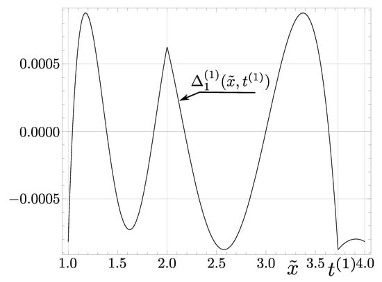
Figure 1.
Graph of the function .
Analogously, we can determine the value of (assuming that is fixed):
Now, the deepest minimum comes from the global maximum:
Therefore, we get:
and the maximum error of the second correction is given by:
which is very close to the value of given by (42).
Thus, we have obtained the algorithm InvSqrt1, see Algorithm 2, which looks like InvSqrt with modified values of the numerical coefficients.
| Algorithm 2:InvSqrt1. |
| 1. float InvSqrt1(float x){ |
| 2. float simhalfnumber = 0.500438180f*x; |
| 3. int i = *(int*) &x; |
| 4. i = 0x5F375A86 - (); |
| 5. y = *(float*) &i; |
| 6. y = y*(1.50131454f - simhalfnumber*y*y); |
| 7. y = y*(1.50000086f - 0.999124984f*simhalfnumber*y*y); |
| 8. return y; |
| 9. } |
Comparing with , we easily see that the number of algebraic operations in is greater by one (an additional multiplication in Line 7, corresponding to the second iteration of the modified Newton–Raphson procedure). We point out that the magic constants for InvSqrt and InvSqrt1 are the same.
5. Numerical Experiments
The new algorithm was tested on the processor Intel Core i5-3470 using the compiler TDM-GCC 4.9.2 32-bit. Using the same hardware for testing the code , we obtained practically the same values of errors as those obtained by Lomont [38]. The same results were obtained also on Intel i7-5700. In this section, we analyze the rounding errors for the code .
Applying algorithm , we obtain relative errors characterized by “oscillations” with a center slightly shifted with respect to the analytical approximate solution ; see Figure 2. The observed blur can be expressed by a relative deviation of the numerical result from :
The values of this error are distributed symmetrically around the mean value :
enclosing the range:
see Figure 3. The blur parameters of the function show that the main source of the difference between analytical and numerical results is the use of precision float and, in particular, rounding of constant parameters of the function . We point out that in this case, the amplitude of the error oscillations is about greater than the amplitude of oscillations of (i.e., in the case of ); see the right part of Figure 2 in [46]. It is worth noting that for the first Newton–Raphson correction, the blur is of the same order, but due to a much higher error value in this case, its effect is negligible (i.e., Figure 1 would be practically the same with or without the blur). The maximum numerical errors practically coincide with the analytical result (53), i.e.,
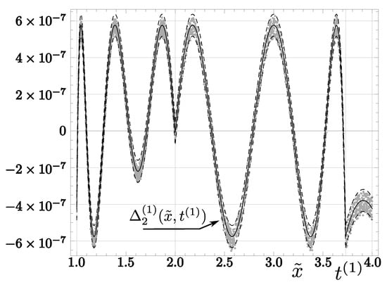
Figure 2.
Solid lines represent function . Its vertical shifts by are denoted by dashed lines. Finally, dots represent relative errors for 4000 random values produced by algorithm .
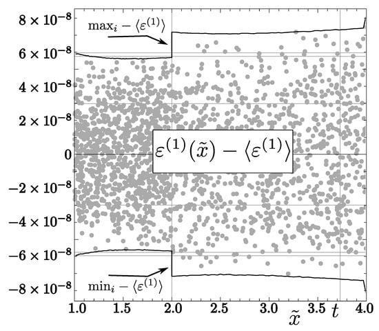
Figure 3.
Relative error arising during the float approximation of corrections . Dots represent errors determined for 2000 random values . Solid lines represent maximum () and minimum () values of relative errors (intervals and were divided into 64 equal intervals, and then, extremum values were determined in all these intervals).
In the case of the second Newton–Raphson correction, we compared results produced by with exact values of the inverse square root for all numbers x of the type float such that . The range of errors was the same for all these intervals (except ):
For , the interval of errors was slightly wider: , which can be explained by the fact that the analysis presented in this paper is not applicable to subnormal numbers; see (1). Therefore, our tests showed that relative errors for all numbers of the type float belong to the interval , where:
These values are significantly higher than the analytical result () (see (57)), but are still much lower than the analogous error for the algorithm (; see [46]).
6. Conclusions
In this paper, we presented a modification of the famous code InvSqrt for fast computation of the inverse square root of single-precision floating-point numbers. The new code had the same magic constant, but the second part (which consisted of Newton–Raphson iterations) was modified. In the case of one Newton–Raphson iteration, the new code InvSqrt1 had the same computational cost as InvSqrt and was two-times more accurate. In the case of two iterations, the computational cost of the new code was only slightly higher, but its accuracy was higher by almost seven times.
The main idea of our work consisted of modifying coefficients in the Newton–Raphson method and demanding that the maximal error be as small as possible. Such modifications can be constructed if the distribution of errors for Newton–Raphson corrections is not symmetric (like in the case of the inverse square root, when they are non-positive functions).
Author Contributions
Conceptualization, L.V.M.; formal analysis, C.J.W.; investigation, C.J.W., L.V.M., and J.L.C.; methodology, C.J.W. and L.V.M.; visualization, C.J.W.; writing, original draft, J.L.C.; writing, review and editing, J.L.C.
Funding
This research received no external funding.
Conflicts of Interest
The authors declare no conflict of interest.
References
- Ercegovac, M.D.; Lang, T. Digital Arithmetic; Morgan Kaufmann: Burlington, MA, USA, 2003. [Google Scholar]
- Parhami, B. Computer Arithmetic: Algorithms and Hardware Designs, 2nd ed.; Oxford University Press: New York, NY, USA, 2010. [Google Scholar]
- Diefendorff, K.; Dubey, P.K.; Hochsprung, R.; Scales, H. AltiVec extension to PowerPC accelerates media processing. IEEE Micro 2000, 20, 85–95. [Google Scholar] [CrossRef]
- Harris, D. A Powering Unit for an OpenGL Lighting Engine. In Proceedings of the 35th Asilomar Conference on Singals, Systems, and Computers, Pacific Grove, CA, USA, 4–7 November 2001; pp. 1641–1645. [Google Scholar]
- Sadeghian, M.; Stine, J. Optimized Low-Power Elementary Function Approximation for Chybyshev series Approximation. In Proceedings of the 46th Asilomar Conference on Signal Systems and Computers, Pacific Grove, CA, USA, 4–7 November 2012. [Google Scholar]
- Russinoff, D.M. A Mechanically Checked Proof of Correctness of the AMD K5 Floating Point Square Root Microcode. Form. Methods Syst. Des. 1999, 14, 75–125. [Google Scholar] [CrossRef]
- Cornea, M.; Anderson, C.; Tsen, C. Software Implementation of the IEEE 754R Decimal Floating-Point Arithmetic. In Software and Data Technologies (Communications in Computer and Information Science); Springer: Berlin/Heidelberg, Germany, 2008; Volume 10, pp. 97–109. [Google Scholar]
- Muller, J.-M.; Brisebarre, N.; Dinechin, F.; Jeannerod, C.-P.; Lefèvre, V.; Melquiond, G.; Revol, N.; Stehlé, D.; Torres, S. Hardware Implementation of Floating-Point Arithmetic. In Handbook of Floating-Point Arithmetic; Birkhäuser: Basel, Switzerland, 2010; pp. 269–320. [Google Scholar]
- Muller, J.-M.; Brisebarre, N.; Dinechin, F.; Jeannerod, C.-P.; Lefèvre, V.; Melquiond, G.; Revol, N.; Stehlé, D.; Torres, S. Software Implementation of Floating-Point Arithmetic. In Handbook of Floating-Point Arithmetic; Birkhäuser: Basel, Switzerland, 2010; pp. 321–372. [Google Scholar]
- Viitanen, T.; Jääskeläinen, P.; Esko, O.; Takala, J. Simplified floating-point division and square root. In Proceedings of the IEEE International Conference on Acoustics Speech and Signal Process, Vancouver, BC, Canada, 26–31 May 2013; pp. 2707–2711. [Google Scholar]
- Ercegovac, M.D.; Lang, T. Division and Square Root: Digit Recurrence Algorithms and Implementations; Kluwer Academic Publishers: Boston, MA, USA, 1994. [Google Scholar]
- Liu, W.; Nannarelli, A. Power Efficient Division and Square root Unit. IEEE Trans. Comp. 2012, 61, 1059–1070. [Google Scholar] [CrossRef]
- Deng, L.X.; An, J.S. A low latency High-throughput Elementary Function Generator based on Enhanced double rotation CORDIC. In Proceedings of the IEEE Symposium on Computer Applications and Communications (SCAC), Weihai, China, 26–27 July 2014. [Google Scholar]
- Nguyen, M.X.; Dinh-Duc, A. Hardware-Based Algorithm for Sine and Cosine Computations using Fixed Point Processor. In Proceedings of the 11th International Conference on Electrical Engineering/Electronics Computer, Telecommuncations and Information Technology, Nakhon Ratchasima, Thailand, 14–17 May 2014. [Google Scholar]
- Cornea, M. Intel® AVX-512 Instructions and Their Use in the Implementation of Math Functions; Intel Corporation, 2015. Available online: http://arith22.gforge.inria.fr/slides/s1-cornea.pdf (accessed on 27 June 2019).
- Jiang, H.; Graillat, S.; Barrio, R.; Yang, C. Accurate, validated and fast evaluation of elementary symmetric functions and its application. Appl. Math. Comput. 2016, 273, 1160–1178. [Google Scholar] [CrossRef]
- Fog, A. Software Optimization Resources, Instruction Tables: Lists of Instruction Latencies, Throughputs and Micro-Operation Breakdowns for Intel, AMD and VIA CPUs. Available online: http://www.agner.org/optimize/ (accessed on 27 June 2019).
- Moroz, L.; Samotyy, W. Efficient floating-point division for digital signal processing application. IEEE Signal Process. Mag. 2019, 36, 159–163. [Google Scholar] [CrossRef]
- Eberly, D.H. GPGPU Programming for Games and Science; CRC Press: Boca Raton, FL, USA, 2015. [Google Scholar]
- Ide, N.; Hirano, M.; Endo, Y.; Yoshioka, S.; Murakami, H.; Kunimatsu, A.; Sato, T.; Kamei, T.; Okada, T.; Suzuoki, M. 2.44-GFLOPS 300-MHz Floating-Point Vector-Processing Unit for High-Performance 3D Graphics Computing. IEEE J. Solid-State Circuits 2000, 35, 1025–1033. [Google Scholar] [CrossRef]
- Oberman, S.; Favor, G.; Weber, F. AMD 3DNow! technology: Architecture and implementations. IEEE Micro 1999, 19, 37–48. [Google Scholar] [CrossRef]
- Kwon, T.J.; Draper, J. Floating-point Division and Square root Implementation using a Taylor-Series Expansion Algorithm with Reduced Look-Up Table. In Proceedings of the 51st Midwest Symposium on Circuits and Systems, Knoxville, TN, USA, 10–13 August 2008. [Google Scholar]
- Hands, T.O.; Griffiths, I.; Marshall, D.A.; Douglas, G. The fast inverse square root in scientific computing. J. Phys. Spec. Top. 2011, 10, A2-1. [Google Scholar]
- Blinn, J. Floating-point tricks. IEEE Comput. Graph. Appl. 1997, 17, 80–84. [Google Scholar] [CrossRef]
- Janhunen, J. Programmable MIMO Detectors. Ph.D. Thesis, University of Oulu, Tampere, Finland, 2011. [Google Scholar]
- Stanislaus, J.L.V.M.; Mohsenin, T. High Performance Compressive Sensing Reconstruction Hardware with QRD Process. In Proceedings of the IEEE International Symposium on Circuits and Systems (ISCAS’12), Seoul, Korea, 20–23 May 2012. [Google Scholar]
- Avril, Q.; Gouranton, V.; Arnaldi, B. Fast Collision Culling in Large-Scale Environments Using GPU Mapping Function; ACM Eurographics Parallel Graphics and Visualization: Cagliari, Italy, 2012. [Google Scholar]
- Schattschneider, R. Accurate High-resolution 3D Surface Reconstruction and Localisation Using a Wide-Angle Flat Port Underwater Stereo Camera. Ph.D. Thesis, University of Canterbury, Christchurch, New Zealand, 2014. [Google Scholar]
- Zafar, S.; Adapa, R. Hardware architecture design and mapping of “Fast Inverse Square Root’s algorithm”. In Proceedings of the International Conference on Advances in Electrical Engineering (ICAEE), Tamilnadu, India, 9–11 January 2014; pp. 1–4. [Google Scholar]
- Hänninen, T.; Janhunen, J.; Juntti, M. Novel detector implementations for 3G LTE downlink and uplink. Analog. Integr. Circ. Sig. Process. 2014, 78, 645–655. [Google Scholar] [CrossRef]
- Li, Z.Q.; Chen, Y.; Zeng, X.Y. OFDM Synchronization implementation based on Chisel platform for 5G research. In Proceedings of the 2015 IEEE 11th International Conference on ASIC (ASICON), Chengdu, China, 3–6 November 2015. [Google Scholar]
- Hsu, C.J.; Chen, J.L.; Chen, L.G. An Efficient Hardware Implementation of HON4D Feature Extraction for Real-time Action Recognition. In Proceedings of the 2015 IEEE International Symposium on Consumer Electronics (ISCE), Madrid, Spain, 24–26 June 2015. [Google Scholar]
- Hsieh, C.H.; Chiu, Y.F.; Shen, Y.H.; Chu, T.S.; Huang, Y.H. A UWB Radar Signal Processing Platform for Real-Time Human Respiratory Feature Extraction Based on Four-Segment Linear Waveform Model. IEEE Trans. Biomed. Circ. Syst. 2016, 10, 219–230. [Google Scholar] [CrossRef] [PubMed]
- Lv, J.D.; Wang, F.; Ma, Z.H. Peach Fruit Recognition Method under Natural Environment. In Eighth International Conference on Digital Image Processing (ICDIP 2016), Chengdu, China, 20–22 May 2016; Falco, C.M., Jaing, X.D., Eds.; SPIE: Bellingham, WA, USA, 2016; Volume 10033, p. 1003317. [Google Scholar]
- Sangeetha, D.; Deepa, P. Efficient Scale Invariant Human Detection using Histogram of Oriented Gradients for IoT Services. In Proceedings of the 2017 30th International Conference on VLSI Design and 2017 16th International Conference on Embedded Systems, Hyderabad, India, 7–11 January 2017; pp. 61–66. [Google Scholar]
- Lin, J.; Xu, Z.G.; Nukada, A.; Maruyama, N.; Matsuoka, S. Optimizations of Two Compute-bound Scientific Kernels on the SW26010 Many-core Processor. In Proceedings of the 46th International Conference on Parallel Processing, Bristol, UK, 14–17 August 2017; pp. 432–441. [Google Scholar]
- Quake III Arena, id Software 1999. Available online: https://github.com/id-Software/Quake-III-Arena/blob/master/code/game/q_math.c#L552 (accessed on 27 June 2019).
- Lomont, C. Fast Inverse Square Root, Purdue University. Tech. Rep.. 2003. Available online: http://www.lomont.org/Math/Papers/2003/InvSqrt.pdf (accessed on 27 June 2019).
- Warren, H.S. Hacker’s Delight, 2nd ed.; Pearson Education: London, UK, 2013. [Google Scholar]
- Martin, P. Eight Rooty Pieces. Overload J. 2016, 135, 8–12. [Google Scholar]
- Robertson, M. A Brief History of InvSqrt. Bachelor’s Thesis, University of New Brunswick, Fredericton, NB, Canada, 2012. [Google Scholar]
- Self, B. Efficiently Computing the Inverse Square Root Using Integer Operations. Available online: https://sites.math.washington.edu/~morrow/336_12/papers/ben.pdf (accessed on 27 June 2019).
- McEniry, C. The Mathematics Behind the Fast Inverse Square Root Function Code. Tech. Rep.. August 2007. Available online: https://web.archive.org/web/20150511044204/http://www.daxia.com/bibis/upload/406Fast_Inverse_Square_Root.pdf (accessed on 27 June 2019).
- Eberly, D. An Approximation for the Inverse Square Root Function. 2015. Available online: http://www.geometrictools.com/Documentation/ApproxInvSqrt.pdf (accessed on 27 June 2019).
- Kornerup, P.; Muller, J.-M. Choosing starting values for certain Newton–Raphson iterations. Theor. Comp. Sci. 2006, 351, 101–110. [Google Scholar] [CrossRef]
- Moroz, L.; Walczyk, C.J.; Hrynchyshyn, A.; Holimath, V.; Cieśliński, J.L. Fast calculation of inverse square root with the use of magic constant—Analytical approach. Appl. Math. Comput. 2018, 316, 245–255. [Google Scholar] [CrossRef]
© 2019 by the authors. Licensee MDPI, Basel, Switzerland. This article is an open access article distributed under the terms and conditions of the Creative Commons Attribution (CC BY) license (http://creativecommons.org/licenses/by/4.0/).