Ultrasonic Assessment of Thickness and Bonding Quality of Coating Layer Based on Short-Time Fourier Transform and Convolutional Neural Networks

Abstract

Ultrasonic non-destructive analysis is a promising and effective method for the inspection of protective coating materials. Offshore coating exhibits a high attenuation rate of ultrasonic energy due to the absorption and ultrasonic pulse echo testing becomes difficult due to the small amplitude of the second echo from the back wall of the coating layer. In order to address these problems, an advanced ultrasonic signal analysis has been proposed. An ultrasonic delay line was applied due to the high attenuation of the coating layer. A short-time Fourier transform (STFT) of the waveform was implemented to measure the thickness and state of bonding of coating materials. The thickness of the coating material was estimated by the projection of the STFT into the time-domain. The bonding and debonding of the coating layers were distinguished using the ratio of the STFT magnitude peaks of the two subsequent wave echoes. In addition, the advantage of the STFT-based approach is that it can accurately and quickly estimate the time of flight (TOF) of a signal even at low signal-to-noise ratios. Finally, a convolutional neural network (CNN) was applied to automatically determine the bonding state of the coatings. The time–frequency representation of the waveform was used as the input to the CNN. The experimental results demonstrated that the proposed method automatically determines the bonding state of the coatings with high accuracy. The present approach is more efficient compared to the method of estimating bonding state using attenuation.

1. Introduction

Coatings are widely applied to offshore structures as corrosion protection layers. Coating layer thinning or lack of adhesion between the coating layer and structure may affect the safety of the structure and ignoring this can result in complete system failure. The lifetime of the coated structure is directly related to the quality of the adhesion of the coating material with the structure. The thickness and adhesion state are two important features of coatings that must be monitored periodically. The thickness of the coating layer relies on the surrounding environment of the structure and the thickness of coatings may vary in different fields of application. In practical applications, the coating is significantly thin and the thickness may vary up to 3 mm. However, in some applications, the coating material is applied as a thin layer on the surface of the metallic structure. In such cases, the thickness of the coating material may be close to 1 mm or even thinner. In the field, the coating material is usually applied by conventional rollers [1] that create many pores on the inside of the polymer. Porosity greatly increases the ultrasonic attenuation of the coating layer, thus ultrasonic testing becomes difficult.

Ultrasound are widely used in the engineering field and can be divided into the cases of using energy and wave propagation. High intensity ultrasound using energy is used in many fields such as cleaning, material processing [2,3,4], and medical therapy [5]. In this case, controls such as initial conditions is key. Ultrasonic measurement using wave propagation is also used in many fields such as non-destructive inspection of structures, quality control of products, sonar, and medical diagnosis. In this case, precise measurement of propagation time and amplitude is key.

Ultrasonic non-destructive technology is widely used in flaw detection and materials evaluation. Piezoelectric transducers that transmit and receive ultrasonic waves have a dead zone called the “main bang” that establishes the pulse–echo test method as unable to detect fast returning echoes [6]. In the case of short propagation times, the reflected echoes are superimposed or buried in the dead zone [7,8,9]. Transducers with higher center frequencies have shorter pulse durations and can be used to solve echo-overlapping problems [10]. Conversely, as high-frequency energy is rapidly attenuated, it cannot be applied to the evaluation of the thickness of the coating layer with large attenuation [11].

The time of flight (TOF) of the echo reflected from the layer boundary is required for ultrasonic pulse–echo testing. The back wall echoes of coating arrive very close to each other and accurate estimation of the TOF of an echo signal is a key issue. Studies have been conducted on the Morlet wavelet and least-squares filters [12], the combination of the Hilbert transform and the non-linear least-squares method [13], the principle of maximum likelihood estimation [14] and the cross-correlation method [15,16], and the ellipse method [17].

The ultrasonic non-destructive evaluation of the state of bonding is particularly important to ensure the long-term protection of coated structures. For this purpose, studies regarding, for example, echo signal parameters and joint strength [18], asphalt separation detection using surface waves [19], the ultrasonic C-scan method [20], and the correlation between guided wave amplitudes [21] have been conducted. In addition, the phase of the echo signal and synthetic aperture focusing technique imaging algorithm [22,23,24], the longitudinal wave velocity variation [25,26], the reflected wave velocity frequency characteristic [27,28], the combination of time–domain waveform and numerical simulation [29,30], the support matching method [31], and a method for comparing damping rates [32] are also areas that have been studied.

The STFT technique splits the signal into multiple sections using a sliding window function along the time axis and Fourier transform is applied to each section of the signal [33]. Several researchers have presented results in the evaluation of the bonding state of the adhesive layer using the STFT. For example, Song et al. [34] evaluated the bonding level between shotcrete and planar rock using STFT analysis with an impact echo test [35]. In contrast, in this study, STFT was used both for the precise thickness estimation and bonding state evaluation using the ultrasonic pulse–echo method.

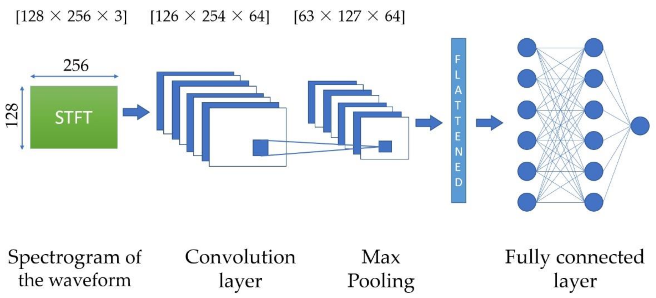
Finally, deep learning algorithms such as convolutional neural networks (CNNs) have been implemented to enable the fast automated identification of the bonding state. Manual inspection of the state of the coating layer is time consuming, expensive, and prone to errors. The detection of the coating layer relies on the amplitude ratio of the ultrasonic wave energy and the presence of the reflected echo signal from the base material. In spite of the significant achievements in the non-destructive inspection of coating layers, most of research results are qualitative and not quantitative. The attenuation-based evaluation of the coating layer presents challenges due to the presence of non-uniform porosity in the layer that causes a variation in the attenuation parameters [36,37].

The purpose of the present study is to develop an advanced ultrasonic assessment system for offshore coatings. An ultrasonic delay line was adopted to separate the reflected back wall echo from the excitation signal (main bang). A short-time Fourier transform (STFT)-based analysis of the waveform has been implemented to estimate the coating layer thickness and bonding state of the coating materials. In addition, STFT spectrogram is integrated with a CNN to provide an automatic classification of the bonding condition of the coating layer. The accuracy and performance of the developed system were evaluated.

2. Short-Time Fourier Transform (STFT)

STFT is a powerful method for analyzing non-stationary signals. Conventional Fourier transform of the signal provides averaged frequency of the signal over an entire time interval. In contrast to the standard Fourier transform, the STFT allows for the representation of the frequency variation of the signal over time. When the STFT method is applied, the signal is divided into equal length sections by the windowing function and the Fourier transform is applied to each section. Using STFT, the continuous time signal $x(u)$ is windowed with a windowing function $h(u)$ to a limited extent and then Fourier transforms are applied. The expression of STFT [38] is illustrated by

$$STFT(t,f)={\displaystyle \underset{-\infty }{\overset{+\infty }{\int }}x(u) h^{*}(u-t) e^{-j2\pi fu}} du$$

(1)

The windowing function is a non-negative and even function with limited duration. In Equation (1), $h^{*}(u)$ is the complex conjugate of the windowing function. The windowing function attempts to reach the peak of the signal and emphasizes it at that instant, while the remaining section of the signal is suppressed by the same window function. Several kinds of window functions exist in the literature: consider Kaiser, Blackman, Gaussian, Nuttall, Chebyshev, and others [39,40]. In the current study, the Gaussian windowing function was applied to STFT analysis and can be defined as [41]

$$h(t)=\left(\frac{1}{\sqrt{2\pi }a}\right)e^{-\frac{1}{2}{\left(\frac{t}{a}\right)}^2}$$

(2)

Gaussian windowing has advantages for the time–frequency representation of the waveform due to its optimal concentration in both the time and frequency domains. The scale factor (or window duration) $a$ in Equation (2) determines the size or duration of the windowing function. The scale factor of the windowing function must be selected carefully because it determines the resolution of both the time and frequency domains. An infinitely fine resolution of time and frequency cannot be obtained simultaneously. To achieve good frequency resolution, a long windowing function is required, whereas a better time resolution is obtained with a short windowing function. The duration of the Gaussian windowing function for optimal resolution of both in time and frequency domain can be computed by [42]

$$a=\sqrt{\frac{\lambda }{2{\pi }^2}}$$

(3)

The reflected echo from the back wall can be described by a Gaussian echo model [42]. The back wall echo model is described in Equation (4) and the parameters of the equation are the following; $\beta$ is the amplitude, $\lambda$ is the bandwidth factor, $f_c$ is the center frequency, $\tau$ is the TOF, and $\varphi$ is the phase of the reflected echo signal.

$$x(t)=\beta e^{(-\lambda {(t-\tau )}^2+j(2\pi f_c(t-\tau )+\varphi ))}$$

(4)

The magnitude of the STFT can be calculated by substituting the model of the back wall echo (Equation (4)) into the STFT expression (Equation (1)) in addition to the Gaussian windowing function (Equation (2)). The simplified expression of the magnitude of the STFT can be defined as [41]

$$|STFT(t,f)|=\frac{\beta }{\sqrt{2\lambda a^2+1}}\exp \left[-\frac{\lambda }{2\lambda a^2+1}{\left(t-\tau \right)}^2-\frac{2{\pi }^2{a}^2}{2\lambda a^2+1}{\left(f-f_c\right)}^2\right]$$

(5)

As evident in Equation (5), the expression of the magnitude of the STFT of the back wall echo model is a function of both time and frequency. The STFT can be represented as a three-dimensional plot where the x, y, and z axes correspond to the time, frequency, and intensity of the STFT magnitude, respectively. Although, useful information can be derived from a two-dimensional view of the STFT (i.e., time–frequency or time–magnitude) as well. By using the obtained magnitude of the STFT, the waveform parameters such as the TOF and center frequency can be estimated. To calculate the TOF of the waveform, the obtained STFT magnitudes must be projected into the time-domain and the local peaks of the projected STFT magnitude into the time-domain $\left(\frac{\partial \left|STFT(t,f)\right|}{\partial t}=0\right)$ correspond to the TOF of the waveform. Similarly, the center frequency of the waveform can be evaluated by estimating $\frac{\partial \left|STFT(t,f)\right|}{\partial f}=0$ of the STFT projection to the frequency domain which corresponds to the central frequency [43].

The magnitude of the STFT shows the distribution of the energy of the waveform over the time–scale plane. The waveform energy $E$ (Equation (6)) distributed over the time–frequency plane can be obtained by integrating the magnitude of the STFT and the relation can be defined as [44,45,46]

$$E={\displaystyle \underset{-\infty }{\overset{+\infty }{\int }}{\displaystyle \underset{-\infty }{\overset{+\infty }{\int }}{\left|STFT(t,f)\right|}^{2}dtdf}}$$

(6)

3. Experiments

3.1. Ultrasonic Echoes from the Coating Layer

Ultrasonic delay lines were used to shift the first echo in the “main bang”. Figure 1 shows the wave propagation patterns of fully bonded and debonded coatings when delay lines are used, where A0 represents the echo reflected between the delay line and the coating, and A1 represents the echo reflected from the back wall of the coating layer. When the coating layer adheres well to the base material, part of the ultrasonic energy is propagated into the base material; thus, the amplitude of the A1 echo becomes smaller than when the coating layer and the base material are separated. When the coating layer is bonded with carbon steel, the A2 corresponds to the back wall echo waveform from the base material, whereas in the debonded layer, A2 is the second echo from the back wall of the coating material.

In this study, the case of debonding and bonding between the coating material and structure was distinguished using the amplitude ratio of the peak STFT magnitude. In reference to Equation (5), the STFT magnitude peak is proportional to the waveform amplitude $\beta$ [47]; thus, the ratio of the STFT magnitude peaks of the two subsequent wave echoes was used to compare the amplitude ratio of the two waveforms.

3.2. Test Sample Preparation

To validate the proposed method in actual experiments, specimens were fabricated using two types of polymer coating materials. Both coating materials are composed of an epoxy resin and a hardener, and detailed information on the two coating materials is presented in

Table 1. Information/Material Properties of the coating materials.

Information/Properties	Epoxy A	Epoxy B
Commercial name	ALOCIT 28.14	RS 500P
Maker	A&E Group	Chemco
Weight ratio (Epoxy resin: hardener)	5:1	5.1:1
Density	1.94 g/cm3	1.67 g/cm3
Ultrasonic wave speed	2.46 $\mathrm{mm}/\mathsf{\mu }\mathrm{s}$	2.40 $\mathrm{mm}/\mathsf{\mu }\mathrm{s}$

[48]. Carbon steel plates with dimensions of 150 mm × 50 mm × 4 mm were used as the base material for both types of coatings.

The epoxy resin and hardener for each coating were mechanically mixed for 3–5 min in separate plastic containers. There are several ways to apply the coating [49] but as is common in the field, it was applied individually to the surface of the base material using conventional rollers. As hand mixing and roller application are used, there are many pores inside the coating layer. They increase attenuation in the coating layer and thus ultrasound examination is difficult.

The surfaces of the carbon steel plates were divided into two parts. In the first part, coating material was directly applied to the surface of the base materials to create a perfect bond between the carbon steel and the coating. In the second part, a thin sheet of stainless steel with a thickness of 0.05 mm was placed between the coating and the base material, and after curing the coated specimen at room temperature, the thin stainless steel sheet was removed. As a result, the coating layer and carbon steel were completely separated and a completely debonded layer of the coating was obtained. The fabricated specimens are shown in Figure 2.

3.3. Experimental Set-Up

Figure 3 illustrates the instrume setup used for the ultrasonic pulse–echo measurements of the specimens. The pulser-receiver (5072 PR, Panametrics, Waltham, MA, USA) was used for the generation and reception of the ultrasound. The digital oscilloscope (WaveRunner 604Zi, Teledyne LeCroy, Chestnut Ridge, NY, USA) was used for averaging and recording the received waveforms. A piezoelectric transducer with a central frequency of 5 MHz was used. A lower frequency transducer generated long-lasting signals that led to the overlapping of the echo waves, whereas at high frequencies, the amplitude ratio was increased. Also, an acrylic delay line of 6.2 mm thick was used.

4. Results and Discussions

4.1. Coating Layer Thickness Measurement

All thickness measurements were performed on the debonded area of the coating layer. The main purpose of this experiment was to measure the thickness of the coating layer and as mentioned in Section 2, the TOF of the wave packet can be determined by the local maximum value of projection of the STFT magnitude into the time-domain. Thickness measurement experiments were performed on coating materials of various thicknesses. In the first step, coatings with a thickness of 1.1–1.5 mm were examined using ultrasound. 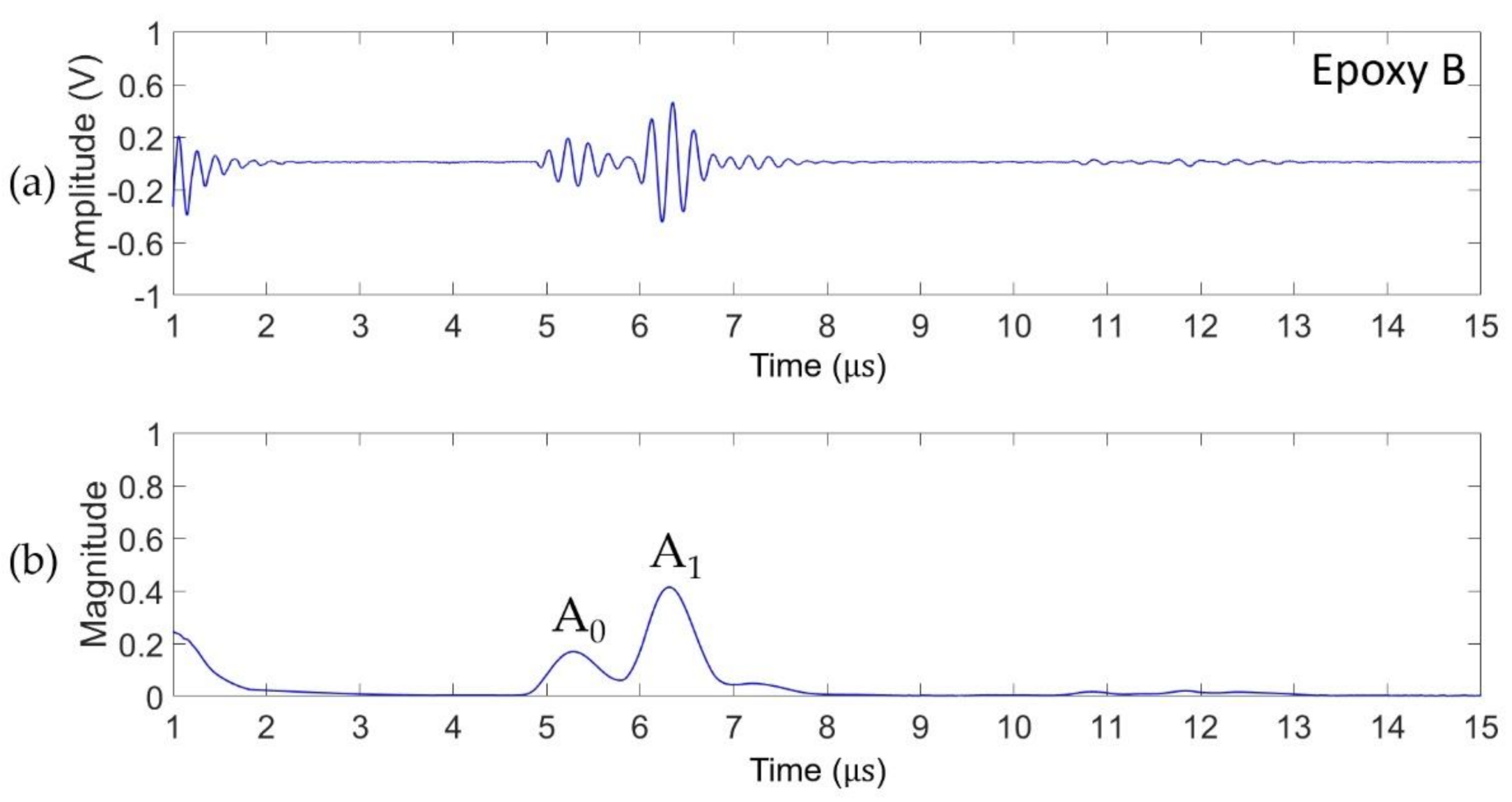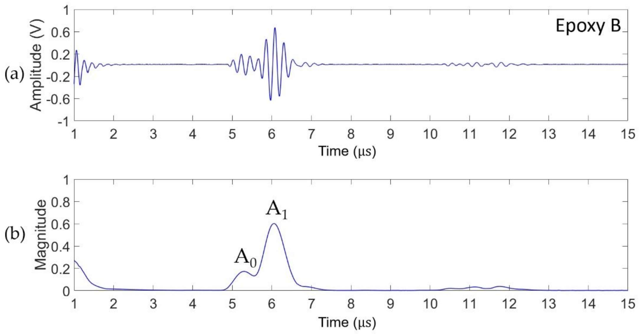Figure 4 and Figure 5 show the experimental results from the direct pulse–echo test of the epoxy A and epoxy B coating layers, respectively.

The peaks of the STFT magnitude can be observed in the figures in which the first echo denoted by A0 is the signal reflected from the boundary between the delay line and the coating layer surface, and the echo denoted by A1 is the signal reflected from the boundary between the base material and the coating material. By knowing the wave velocity in the coating and the TOF difference of the two echoes, the thickness of the coating layer is calculated.

The difference in acoustic impedance of the delay line and the coating material causes the larger magnitude of the A1 echo compared to the A0, as shown in Figure 5. More precisely, the acoustic impedances of epoxy A and B are 4.77 × 10⁶ kg/(m²s) and 4.01 × 10⁶ kg/(m²s), respectively, which is similar to the acoustic impedance of the acrylic delay line (3.26 × 10⁶ kg/(m²s)). This is because the transmitted energy is greater than the reflected energy at the interface.

In epoxy A, the longitudinal wave velocity is 2.46 mm/μs, the TOF of the first wave echo obtained in Figure 4b is 5.28 μs, and the arrival time of the next echo is 6.40 μs; thus, the thickness of the coating layer is 1.38 mm. Similarly, the longitudinal wave velocity of epoxy B is 2.40 mm/μs and the corresponding TOFs for echoes A0 and A1 are 5.28 μs and 6.31 μs, respectively; thus, the thickness was estimated to be 1.24 mm.

The experiment was repeated with thinner layers of the epoxy A and B coatings and the STFT-based method was applied to the obtained waveforms; the results are shown in Figure 6 and Figure 7. By the above method, the thicknesses of the epoxy A and B coatings were estimated to be 0.91 mm and 0.92 mm, respectively.

Measurement data using ultrasound was verified by a manual measurement using calipers. Repeatability was checked by measuring five times the same thickness by each method and the standard deviation (std dev.) was calculated; values are shown in

Table 2. Coating layer thickness measurements by caliper and ultrasound.

Coating Material	Thickness Measured by Caliper		Thickness Measured by Ultrasound		Error
	(Average)	(Std Dev.)	(Average)	(Std Dev.)
Epoxy A	1.37 mm	0.0074	1.38 mm	0.0040	0.7%
Epoxy A	0.92 mm	0.0075	0.91 mm	0.0070	1.1%
Epoxy B	1.25 mm	0.0040	1.24 mm	0.0108	0.8%
Epoxy B	0.91 mm	0.0109	0.92 mm	0.0045	1.1%

. Comparing the thickness values measured with both methods showed similar results and the difference between the two values was about 1%.

The thickness of the coating layer was measured by applying the STFT which was able to accurately measure the thickness of less than 1 mm for both types of coating materials. Although the TOF of the reflected echo can be evaluated from the time-domain waveform, the advantage of the STFT-based approach is that it can accurately and quickly estimate the TOF of the signal even at low signal-to-noise ratios.

4.2. Evaluation of Bonding Status

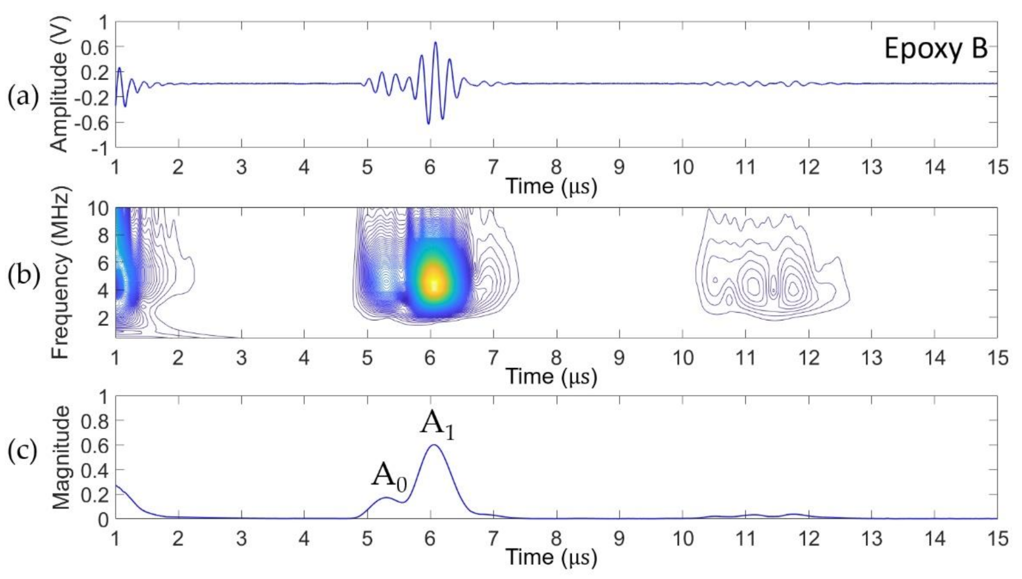
In order to evaluate the bonding state between the coating layer and the base material, ultrasonic experiments were performed on the bonded and debonded parts, and the results are shown in Figure 8 and Figure 9, respectively. The received time–domain waveform is presented in (a) and (b) presents the time–frequency representation obtained using STFT which is used as an input signal for the CNN that will be mentioned later. In addition, (c) presents the magnitude of the projected STFT in the time-domain, allowing for the accurate estimation of the TOF of the echo. Similarly, Figure 10 and Figure 11 present the results measured for the perfectly bonded and debonded portions of the epoxy B specimen, respectively.

Parameters of the received waveform such as the TOF and magnitude of the STFT of bonded sections of epoxy A and B are listed in

Table 3. Estimated properties of the signal from a perfectly bonded and debonded layer of epoxy A.

Perfectly Bonded
Order of Echo	TOF [µs]	∆TOF [µs]	Magnitude of STFT
A0	$t_1=5.26$		0.21
A1	$t_2=6.02$	$∆t_{21}=0.76$	0.48
A2	$t_3=7.35$	$∆t_{32}=1.33$	0.07
A3	$t_4=8.68$	$∆t_{43}=1.33$	0.06
Debonded
A0	$t_1=5.26$		0.21
A1	$t_2=6.02$	$∆t_{21}=0.76$	0.62

and

Table 4. Estimated properties of the signal from a perfectly bonded and debonded coating layer of epoxy B.

Perfectly Bonded
Order of Echo	TOF [µs]	∆TOF [µs]	Magnitude of STFT
A0	$t_1=5.26$		0.17
A1	$t_2=6.09$	$∆t_{21}=0.83$	0.47
A2	$t_3=7.42$	$∆t_{32}=1.33$	0.11
A3	$t_4=8.75$	$∆t_{43}=1.33$	0.09
Debonded
A0	$t_1=5.26$		0.17
A1	$t_2=6.09$	$∆t_{21}=0.83$	0.60

. The coating layer has relatively high damping due to the presence of porosity inside but the base material is carbon steel with a low damping rate. At the interface between the coating and the substrate, part of the ultrasound is transmitted from the coating to the substrate and the remainder is reflected back towards the ultrasonic transducer (Echo A1). Ultrasonic waves transmitted to the base material return to the transducer after being reflected several times in the base material (Echo A2 and A3).

In the case of the debonded layer, air exists between the base material and the coating film, and almost all of the ultrasonic waves are reflected from the back wall of the coating and reach the ultrasonic transducer (Echo A1).

The amplitude of the first echo (A0) which is reflected off the back wall of the delay line is the same for both the bonded and debonded conditions. The bond between the coating layer and the base material transmits a certain amount of ultrasonic energy from the coating material to the base material, reducing the size of the A1 echo. Therefore, the ratio of the two echoes (A1/A0) can be used to evaluate the bonding state of the coating layer. In the case of a perfectly bonded specimen, A1/A0 = 2.28, which is smaller than A1/A0 = 2.95 if not bonded. Similarly, in the case of the epoxy B specimen, the bonded specimen is A1/A0 = 2.76, which is smaller than A1/A0 = 3.53 in the case of the unbonded specimen.

Goglio et al. obtained similar results [50]. They observed that the rate of amplitude decay of the ultrasonic echoes was faster in layer with adhesions compared to the layer without adhesions. However, ultrasonic detection of the debonding state of the coating layer must consider complex situations such as delay lines, acoustic impedance mismatch between the coating material and the base materials, high attenuation of the coating material, various thicknesses of the coating layer, and waveform mixing between reflected and transmitted echoes. In addition, the ultrasonic echo ratio comparison technique is performed manually and the peak ratio of the STFT magnitudes depends on several parameters of the material properties of both the coating and the delay line. To overcome this, a CNN was used to automatically and quickly detect the bonding state of the coating layer.

5. Artificial Neural Network

We propose a combined technique of the STFT spectrogram with a CNN for automatically classifying the state of the coating layers. CNNs are a class of deep learning networks [51]. In contrast to traditional neural networks, CNNs contain feature extracting convolutional and pooling layers with a local connection. Direct implementation of neural networks for coating material classification can lead to the usage of many parameters and is therefore a time-consuming training process [52].

5.1. Structure of CNN

The structure of the CNN consists of several layers including the convolutional layer, activation layer, pooling layer, and fully connected layer [53]. Figure 12 shows the architecture of the CNN used in this study. As can be observed from the figure, the CNN structure consists of convolution, pooling, and fully connected layers. Initially, the time–frequency representation of the waveform is computed using STFT and then the 2D image of the spectrogram is used as an input to the convolutional layer of the CNN. The hyperparameters that determine the CNN structure are classified into two types: network structure hyperparameters and trained network hyperparameters. The kernel type, kernel size, padding, stride, and activation function correspond to network structure parameters. The training network parameters are learning rate, momentum, epoch number, and batch size.

The convolution layer consists of kernel filters that require significant computational resources compared with other layers. In our model, the convolutional layer had a total of 64 filters with dimensions of 3 × 3. Low resolution images are formed by kernel filters that are called a feature map. As an activation function of the convolution layer, a rectified linear unit (ReLU) was used. The applied ReLU activation function is to normalize the input image and increase the non-linearity of the convolutional layer output. The output of the ReLU function is zero when it receives a zero or negative value, while the positive values are kept unchanged. The ReLU activation function is defined as [54]

$$f(x)=\left\{\begin{array}{l}0 \mathrm{if} x\le 0\\ x \mathrm{if} x>0\end{array}\right\}$$

(7)

In the pooling layer, max-pooling was applied with a kernel size of 2 × 2 and the stride was equal to two. The feature maps are further downsized by the pooling layer and then were flattened. In the flattening process, all matrices are reordered in a column and were used as the input of the fully connected layer. The fully connected layer consists of several neurons and each neuron generates a single output (0 or 1) while having single or multiple inputs. The input of the neuron is associated with a weight and its value is directly related to the importance of the input value. In the designed CNN, the output of the fully connected layer belonged to a single neuron that was based on the sigmoid activation function. Because the applied CNN model output required to be binary classified the state o bonding of the coating layer whether to bonded or debonded condition of the layer.

The original spectrogram image has 768 × 1536 pixels. Spectrogram images were downsized to 128 × 256 pixels and were applied for the training of the CNN.

Table 5. Specification of the model architecture.

Layer Type	Output Shape
Input layer	128 × 256 × 3
Convolution layer	126 × 254 × 64
Max pooling	63 × 127 × 64
Flattening	512,064
Fully connected layer	512
Predictions	2

summarizes the details of the output feature sizes of the CNN layers. During the training of the CNN, the Adam (adaptive moment estimation) algorithm was implemented as an optimizer and the learning rate was set to 0.003. The binary cross-entropy function was used as a loss function. The parameter of the CNN is summarized in

Table 6. CNN structure hyperparameters.

Hyperparameters of the CNN
Learning algorithm	Adam
Non-linearity activation function	ReLU
Activation function	Sigmoid
Number of epochs	30
Learning rate	0.003
Number of filters	64
Kernel size	3 × 3
Batch size	32
Momentum	0.9

. The parameters of the CNN could be further optimized until optimal values are reached by using boosting algorithms. In the literature, three several known boosting methods are presented [55]: AdaBoost [56], XGBoosting [57], and Gradient boosting [58], among others. For example, Bustillo et al. [59] implemented AdaBoost ensembles to optimize the parameters of neural networks for data extraction features from tests and to improve the accuracy of prediction to 5%. In general, when the prediction accuracy by a neural network is low, the parameters of the neural network are optimized, and the optimization can affect the overall accuracy and performance of the neural networks. However, optimization parameters of the CNN require significant computation resources and optimal parameter settings that are beyond the scope of this study.

The main advantage of the CNN concerns the presence of a feature extracting layer in the structure. This allows for the direct use of the spectrograms as the input of the CNN without any additional processing. However, the disadvantage of the CNN concerns the large number of hyperparameters that significantly affect the performance of CNNs. Apart from the many algorithms of optimizing hyperparameters, there is a limit to establishing an optimal combination of all parameters of the CNN. In most cases, main hyperparameters are set manually by trial and error.

5.2. Results of the CNN

In a method to classify the bonding state of a coating material based on the amplitude of the ultrasonic echo, the peak ratio of the STFT magnitudes depends on several parameters of the material properties of the coating and delay lines. To solve this problem, the CNN was developed to automatically and quickly classify the bonding state of the coating layer. The Keras library was used to build the proposed CNN model and it was applied to both types of coating materials. In addition, ultrasonic measurements were recorded on several samples of bonded and debonded sections of both types of coating materials. A total of 4400 ultrasonic inspections were performed on both coating materials (epoxies A and B) with a uniform thickness of the coating layer. Among overall measurements, 2000 were conducted on the bonded sections of the specimens and the remaining 2200 tests were conducted on the completely debonded sections. The spectrogram of each measured waveform was calculated by applying STFT and 2D image of spectrogram was used as an input of the CNN model. The spectrogram representation was implemented in a subset for the training, validation, and testing of the CNN model. The CNN model was trained separately for the epoxy A and epoxy B type of coating for 30 epochs and individual performance was evaluated for each type of coating material. The sizes of the used subset of both the epoxy A and epoxy B types of materials are listed in

Table 7. Distribution of the dataset.

Epoxy A
Bonding condition	Training set	Validation set	Test set	Total
Perfectly bonded	1000	400	600	2000
Debonded	1200	400	600	2200
Epoxy B
Bonding condition	Training set	Validation set	Test set	Total
Perfectly bonded	1000	400	600	2000
Debonded	1200	400	600	2200

.

Figure 13a,b present the training and validation accuracy trends for epoxy A and epoxy B materials, respectively. Both two curves (Figure 13a,b) demonstrate an increasing tendency of training and validation accuracy with epoch iterations. The trend of the graphs does not show significant oscillation of accuracy over epochs and neither graph does not show significant overfitting or underfitting signs. Then, by applying the trained model on the testing subsets, the confusion matrix was plotted for the epoxy A and epoxy B coating material as shown in Figure 13c,d, respectively.

In this study, the accuracy of the test subset in the confusion matrix is defined by Equation (8):

$$Accuracy=\frac{CC}{CC+IC} 100\%$$

(8)

where $CC$ indicates correct classified values and $IC$ is incorrect classified values. As evident from the confusion matrix shown in Figure 13b,c, the proposed method provides high accuracy for both types of coating materials. For example, the accuracy of the correct classification of the debonded coating material was 99.67% for the epoxy A type coating material, whereas for epoxy B it was 99.50%. Similarly, correct detection of the bonded section of the coating material was also high for both types of coating materials: 99.83% for epoxy A and 99.33% for epoxy B. However, there was a minor error rate of 0.33% by classifying the bonded section as debonded for epoxy A and 0.50% for epoxy B.

As shown in Figure 8b and Figure 10b, echoes A2 and A3 are reflected from the back wall of the base material to the coating layer. In the spectrogram of the waveform from the bonded layer, echoes A2 and A3 appear, although they do not appear in the debonded coating layer (in Figure 9b and Figure 11b). This feature allows the CNN to classify the bonded and debonded layer with high accuracy. According to the confusion matrix, it can be seen that the CNN model was classifying with over 99% accuracy of bonded and debonded layer for both types of coating materials.

6. Conclusions

In this study, the STFT method was presented to measure the thickness and bonding state of the coating layer. We also trained a CNN with STFT spectrograms and automatically detected the bonding state of the coating layers using the trained model. Based on the results, the following conclusions can be drawn:

• The delay line allows for the measuring of the thickness of the coating layer with a single echo from the back wall of the coating layer. The magnitude projection of the STFT allowed for a more accurate measurement of the thickness of the coating material. When comparing the ultrasonic measurement result with the thickness value measured with a caliper, similar results were found and the difference between the two values was about 1%.
• Although the TOF of the reflected echo can also be evaluated on time–domain waveforms, the advantage of the STFT-based approach concerns the fact that it can accurately and quickly estimate the TOF of a signal even at low signal-to-noise ratios.
• The ratio of STFT magnitude peaks between two sequential echoes A1 and A0 show a clear difference between the bonded and debonded coatings. The ratio of the STFT size peaks was larger in the case of debonding than in the case of the bonded coating layer. It was also established that the debonded coating layer can be confirmed regardless of the coating material.
• It is possible and effective to detect the debonded coating layer based on the spectrogram of the waveform and the CNN. The applied CNN-based approach has been shown to accurately classify the bonded and debonded states of coating layers with greater than 99% accuracy. Based on this study, the thickness and bonding state of the coating layer can be easily determined through a combination of the spectrogram of the waveform and a CNN. The proposed method can be quickly implemented on other types of coating materials. Further optimization of the design parameters will be performed in future studies.

References

1. Kim, S.; Hong, H.; Han, T.H.; Kim, M.O. Early-age tensile bond characteristics of epoxy coatings for underwater applications. Coatings 2019, 9, 757. [Google Scholar] [CrossRef] [Green Version]
2. Celaya, A.; Lacalle, L.N.L.; Campa, F.J.; Lamikiz, A. Ultrasonic assisted turning of mild steels. Int. J. Mater. Prod. Technol. 2010, 37, 60–70. [Google Scholar] [CrossRef]
3. Aurrekoetxea, M.; López de Lacalle, L.N.; Llanos, I. Machining stresses and initial geometry on bulk residual stresses characterization by on-machine layer removal. Materials 2020, 13, 1445. [Google Scholar] [CrossRef] [Green Version]
4. Fitzka, M.; Mayer, H. Variable amplitude testing of 2024-T351 aluminum alloy using ultrasonic and servo-hydraulic fatigue testing equipment. Procedia Eng. 2015, 101, 169–176. [Google Scholar] [CrossRef] [Green Version]
5. Kennedy, J.E. High-intensity focused ultrasound in the treatment of solid tumours. Nat. Rev. Cancer 2005, 5, 321–327. [Google Scholar] [CrossRef] [PubMed]
6. Carlson, J.E.; Ranefjard, S.; Trulsson, F. A subspace based method for near transducer interference suppression. In Proceedings of the 2018 IEEE International Ultrasonics Symposium (IUS), Kope, Japan, 22 October 2018. [Google Scholar] [CrossRef]
7. Kazys, R.; Mudge, P.J.; Sanderson, R.; Ennaceur, C.; Gharaibeh, Y.; Mazeika, L.; Maciulevicius, A. Development of ultrasonic guided wave techniques for examination of non-cylindrical components. Phys. Procedia 2010, 3, 833–838. [Google Scholar] [CrossRef] [Green Version]
8. Huang, Y.; Turner, J.A.; Song, Y.; Ni, P.; Li, X. Enhanced ultrasonic detection of near-surface flaws using transverse-wave backscatter. Ultrasonics 2019, 98, 20–27. [Google Scholar] [CrossRef]
9. Wöckel, S.; Hempel, U.; Weser, R.; Wessely, B.; Auge, J. Particle characterization in highly concentrated suspensions by ultrasound scattering method. Procedia Eng. 2012, 47, 582–585. [Google Scholar] [CrossRef] [Green Version]
10. Cowell, D.M.J.; Freear, S. Separation of overlapping linear frequency modulated (LFM) signals using the fractional fourier transform. IEEE Trans. Ultrason. Ferroelectr. Freq. Control. 2010, 57, 2324–2333. [Google Scholar] [CrossRef] [Green Version]
11. Greenwood, M.S.; Adamson, J.D.; Bamberger, J.A. Long-path measurements of ultrasonic attenuation and velocity for very dilute slurries and liquids and detection of contaminates. Ultrasonics 2006, 44, e461–e466. [Google Scholar] [CrossRef]
12. Chen, H.; Zuo, M.J.; Wang, X.; Hoseini, M.R. An adaptive Morlet wavelet filter for time-of-flight estimation in ultrasonic damage assessment. Measurement 2010, 43, 570–585. [Google Scholar] [CrossRef]
13. Lu, Z.; Yang, C.; Qin, D.; Luo, Y.; Momayez, M. Estimating ultrasonic time-of-flight through echo signal envelope and modified gauss newton method. Measurement 2016, 94, 355–363. [Google Scholar] [CrossRef]
14. Demirli, R.; Saniie, J. Model-based estimation of ultrasonic echoes. Part I: Analysis and algorithms. IEEE Trans. Ultrason. Ferroelectr. Freq. Control. 2001, 48, 787–802. [Google Scholar] [CrossRef]
15. Nandi, A.K. On the subsample time delay estimation of narrowband ultrasonic echoes. IEEE Trans. Ultrason. Ferroelectr. Freq. Control. 1995, 42, 993–1001. [Google Scholar] [CrossRef]
16. Grennberg, A.; Sandell, M. Estimation of subsample time delay differences in narrowband ultrasonic echoes using the Hilbert transform correlation. IEEE Trans. Ultrason. Ferroelectr. Freq. Control. 1994, 41, 588–595. [Google Scholar] [CrossRef] [Green Version]
17. Li, P.; Chen, S.; Cai, Y.; Chen, J.; Li, J. Accurate TOF measurement of ultrasonic signal echo from the liquid level based on a 2-D image processing method. Neurocomputing 2016, 175, 47–54. [Google Scholar] [CrossRef]
18. Ehrhart, B.; Bockenheimer, C. Methods for the quality assessment of adhesive bonded CFRP structures—A resume. In Proceedings of the 2nd International Symposium on NDT in Aerospace, Hamburg, Germany, 22–24 November 2010. [Google Scholar]
19. Ozen, F.S.; Celaya, M.; Nazarian, S.; Saltan, M. Assesment of deflection-based and seismic non-destructive methods to identify delamination of HMA pavements. J. Innov. Transp. 2020, 1, 1103–1110. [Google Scholar]
20. Amenabar, I.; Mendikute, A.; López-Arraiza, A.; Lizaranzu, M.; Aurrekoetxea, J. Comparison and analysis of non-destructive testing techniques suitable for delamination inspection in wind turbine blades. Engineering 2011, 42, 1298–1305. [Google Scholar] [CrossRef]
21. He, J.; Guan, X.; Peng, T.; Liu, Y.; Saxena, A.; Celaya, J.; Goebel, K. A multi-feature integration method for fatigue crack detection and crack length estimation in riveted lap joints using lamb waves. Smart Mater. Struct. 2013, 22, 105007. [Google Scholar] [CrossRef]
22. Mayer, K.; Langenberg, K.J.; Krause, M.; Milmann, B.; Mielentz, F. Characterization of reflector types by phase-sensitive ultrasonic data processing and imaging. J. Nondestr. Eval. 2008, 27, 35–45. [Google Scholar] [CrossRef]
23. Mayer, K.; Ibrahim, M.; Krause, M.; Schubert, M.; Kassel, U. Requirements for a small size ultrasonic imaging system for inspection of concrete elements. In Proceedings of the 19th World Conference on Non-Destructive Testing, Munich, Germany, 13–17 June 2016. [Google Scholar]
24. Mayer, K.; Chinta, P.K.; Langenberg, K.J.; Krause, M. Ultrasonic imaging of defects in known anisotropic and inhomogeneous structures with fast synthetic aperture methods. In Proceedings of the 18th World Conference on Non-Destructive Testing, Durban, South Africa, 16–20 April 2012. [Google Scholar]
25. Norambuena-Contreras, J.; Castro-Fresno, D.; Vega-Zamanillo, A.; Celaya, M.; Lombillo-Vozmediano, I. Dynamic modulus of asphalt mixture by ultrasonic direct test. NDT E Int. 2010, 43, 629–634. [Google Scholar] [CrossRef]
26. Cerniglia, D.; Pantano, A.; Montinaro, N. 3D simulations and experiments of guided wave propagation in adhesively bonded multi-layered structures. NDT E Int. 2010, 43, 527–535. [Google Scholar] [CrossRef]
27. Kamimura, T.; Yoshida, S.; Sasaki, T. Evaluation of ultrasonic bonding strength with optoacoustic methods. Appl. Sci. 2018, 8, 1026. [Google Scholar] [CrossRef] [Green Version]
28. Khalil, A.A.; Kagho, A.N. Non-destructive testing of adhesively bonded joints using vibrational analysis. Int. J. Adhes. Adhes. 1991, 11, 121–127. [Google Scholar] [CrossRef]
29. Titov, S.A.; Maev, R.G.; Bogachenkov, A.N. Pulse-echo NDT of adhesively bonded joints in automotive assemblies. Ultrasonics 2008, 48, 537–546. [Google Scholar] [CrossRef]
30. Xing, L.; Cui, H.L.; Shi, C.; Zhang, Z.; Zhang, J.; Chang, T.; Wei, D.; Du, C.; Zhang, S.; Zhou, Z. Nondestructive examination of polymethacrylimide composite structures with terahertz time-domain spectroscopy. Polym. Test. 2017, 57, 141–148. [Google Scholar] [CrossRef]
31. Mor, E.; Aladjem, M.; Azoulay, A. A sparse approximation method for ultrasonic monitoring the degradation of adhesive joints. NDT E Int. 2018, 98, 17–26. [Google Scholar] [CrossRef]
32. Guyott, C.C.H.; Cawley, P. The ultrasonic vibration characteristics of adhesive joints. J. Acoust. Soc. Am. 1988, 83, 632–640. [Google Scholar] [CrossRef]
33. Xu, K.; Ta, D.; Wang, W. Multiridge-based analysis for separating individual modes from multimodal guided wave signals in long bones. IEEE Trans. Ultrason. Ferroelect. Freq. Contr. 2010, 57, 2480–2490. [Google Scholar] [CrossRef]
34. Song, K.I.; Cho, G.C. Numerical study on the evaluation of tunnel shotcrete using the Impact-Echo method coupled with Fourier transform and short-time Fourier transform. Int. J. Rock Mech. Min. Sci. 2010, 47, 1274–1288. [Google Scholar] [CrossRef]
35. Yi, W.; Jang, C.S.; Han, J.Y.; Kim, M.G. Nondestructive evaluation of adhesively bonded joints using ultrasonic technique. Key Eng. Mater. 2004, 270, 1833–1838. [Google Scholar] [CrossRef]
36. Cox, R.L.; Almond, D.P.; Reiter, H. Ultrasonic attenuation in plasma-sprayed coating materials. Ultrasonics 1981, 19, 17–22. [Google Scholar] [CrossRef]
37. Lin, L.; Zhang, W.; Ma, Z.; Lei, M. Porosity estimation of abradable seal coating with an optimized support vector regression model based on multi-scale ultrasonic attenuation coefficient. NDT E Int. 2020, 113, 102272. [Google Scholar] [CrossRef]
38. Auger, F.; Flandrin, P. Improving the readability of time-frequency and time-scale representations by the reassignment method. IEEE Trans. Signal. Process. 1995, 43, 1068–1089. [Google Scholar] [CrossRef] [Green Version]
39. Stankovic, L. On the STFT inversion redundancy. IEEE Trans. Circuits Syst. II 2016, 63, 284–288. [Google Scholar] [CrossRef]
40. Bu, Y.; Liu, X.; Turner, J.A.; Song, Y.; Li, X. Grain size evaluation with time-frequency ultrasonic backscatter. NDT E Int. 2021, 117, 102369. [Google Scholar] [CrossRef]
41. Lu, Z.; Ma, F.; Yang, C.; Chang, M. A Novel method for estimating time of flight of ultrasonic echoes through short-time Fourier transforms. Ultrasonics 2020, 103, 106104. [Google Scholar] [CrossRef]
42. Mateo, C.; Talavera, J.A. Short-time Fourier transform with the window size fixed in the frequency domain. Digit. Signal Process. 2018, 77, 13–21. [Google Scholar] [CrossRef]
43. Demirli, R.; Saniie, J. Model-based estimation of ultrasonic echoes. Part II: Nondestructive evaluation applications. IEEE Trans. Ultrason. Ferroelect. Freq. Control. 2001, 48, 803–813. [Google Scholar] [CrossRef] [PubMed]
44. Liu, T.; Li, J.; Cai, X.; Yan, S. A time-frequency analysis algorithm for ultrasonic waves generating from a debonding defect by using empirical wavelet transform. Appl. Acoust. 2018, 131, 16–27. [Google Scholar] [CrossRef]
45. Rioul, O.; Flandrin, P. Time-scale energy distributions: A general class extending wavelet transforms. IEEE Trans. Signal. Process. 1992, 40, 1746–1757. [Google Scholar] [CrossRef]
46. Zhang, Z.; Ren, Y. Time–frequency analysis of echoes signal in ultrasonic testing of adhesion based on short-time Fourier transformation. In Proceedings of the 2010 International Conference on Measuring Technology and Mechatronics Automation, Changsha, China, 13–14 March 2010. [Google Scholar] [CrossRef]
47. Zheng, S.; Zhang, S.; Luo, Y.; Xu, B.; Hao, W. Nondestructive analysis of debonding in composite/rubber/rubber structure using ultrasonic pulse-echo method. Nondestruct. Test. Eval. 2020, 1, 1–13. [Google Scholar] [CrossRef]
48. Won, B.; Kim, M.O.; Park, S.; Yi, J.-H. Effects of water exposure on the interfacial bond between an epoxy resin coating and a concrete substrate. Materials 2019, 12, 3715–3726. [Google Scholar] [CrossRef] [PubMed] [Green Version]
49. Kim, S.; Hong, H.; Park, J.K.; Park, S.; Choi, S.I.; Kim, M.O. Effect of exposure conditions on the interfacial bond properties of SS400 plate coated with various epoxy resins. Coatings 2020, 10, 1159. [Google Scholar] [CrossRef]
50. Goglio, L.; Rossetto, M. Ultrasonic testing of adhesive bonds of thin metal sheets. NDT E Int. 1999, 32, 323–331. [Google Scholar] [CrossRef]
51. Cheng, G.; Yang, C.; Yao, X.; Guo, L.; Han, J. When deep learning meets metric learning: Remote sensing image scene classification via learning discriminative CNNs. IEEE Trans. Geosci. Remote Sens. 2018, 56, 2811–2821. [Google Scholar] [CrossRef]
52. Miao, R.; Gao, Y.; Ge, L.; Jiang, Z.; Zhang, J. Online defect recognition of narrow overlap weld based on two-stage recognition model combining continuous wavelet transform and convolutional neural network. Comput. Ind. 2019, 112, 103115. [Google Scholar] [CrossRef]
53. Albawi, S.; Mohammed, T.A.; Al-Zawi, S. Understanding of a convolutional neural network. In Proceedings of the 2017 International Conference on Engineering and Technology (ICET), Akdeniz University, Antalya, Turkey, 21–23 August 2017. [Google Scholar] [CrossRef]
54. Nair, V.; Hinton, G.E. Rectified linear units improve restricted boltzmann machines. In Proceedings of the 27th International Conference on Machine Learning, Haifa, Israel, 21 June 2010; Fürnkranz, J., Joachisms, T., Eds.; Omnipress: Madison, WI, USA, 2010. [Google Scholar]
55. Weldegebriel, H.T.; Liu, H.; Haq, A.U.; Bugingo, E.; Zhang, D. A new hybrid convolutional neural network and eXtreme gradient boosting classifier for recognizing handwritten Ethiopian characters. IEEE Access 2020, 8, 17804–17818. [Google Scholar] [CrossRef]
56. Taherkhani, A.; Cosma, G.; McGinnity, T.M. AdaBoost-CNN: An adaptive boosting algorithm for convolutional neural networks to classify multi-class imbalanced datasets using transfer learning. Neurocomputing 2020, 404, 351–366. [Google Scholar] [CrossRef]
57. Thongsuwan, S.; Jaiyen, S.; Padcharoen, A.; Agarwal, P. ConvXGB: A new deep learning model for classification problems based on CNN and XGBoost. Nucl. Eng. Technol. 2021, 53, 522–531. [Google Scholar] [CrossRef]
58. Sudakov, O.; Burnaev, E.; Koroteev, D. Driving digital rock towards machine learning: Predicting permeability with gradient boosting and deep neural networks. Comput. Geosci. 2019, 127, 91–98. [Google Scholar] [CrossRef] [Green Version]
59. Bustillo, A.; Urbikain, G.; Perez, J.M.; Pereira, O.M.; Lopez de Lacalle, L.N. Smart optimization of a friction-drilling process based on boosting ensembles. J. Manuf. Syst. 2018, 48, 108–121. [Google Scholar] [CrossRef]
Figure 1. Schematics of the waveform path: (a) perfectly bonded and (b) debonded case between the coating and base material.
Coatings 11 00909 g001
Figure 2. Fabricated specimens of the coating layers: (a) epoxy A (b) epoxy B.
Coatings 11 00909 g002
Figure 3. Experimental set-up: (1) computer; (2) Lecroy oscilloscope; (3) pulser receiver; (4) piezoelectric transducer; (5) acrylic delay line; and (6) specimen.
Coatings 11 00909 g003
Figure 4. Epoxy A coating layer with a thickness less than 1.5 mm: (a) time-domain waveform and (b) the projection of the STFT of the waveform into the time-domain.
Coatings 11 00909 g004
Figure 5. Epoxy B coating (thickness less than 1.5 mm): (a) time-domain waveform and (b) the projection of the STFT.
Coatings 11 00909 g005
Figure 6. Pulse-echo test of the epoxy A coating layer with a thickness less than 1 mm: (a) time–domain waveform and (b) the projection of the STFT of the waveform.
Coatings 11 00909 g006
Figure 7. Epoxy B coating (thickness less than 1 mm): (a) time-domain waveform and (b) the projection of the STFT.
Coatings 11 00909 g007
Figure 8. Ultrasonic signal from the perfectly bonded sections of the epoxy A: (a) time-domain waveform, (b) time-frequency representation of the waveform, and (c) the projection of STFT of the waveform into the time-domain.
Coatings 11 00909 g008
Figure 9. Experimental result of the debonded epoxy A coating layer: (a) time-domain signal, (b) spectrogram, and (c) the STFT magnitude projection.
Coatings 11 00909 g009
Figure 10. Ultrasonic signal from the pulse-echo experimental result of the perfectly bonded section of epoxy B: (a) time-domain waveform, (b) time-frequency representation, and (c) the projection of the STFT.
Coatings 11 00909 g010
Figure 11. Debonded layer of epoxy B coating: (a) time-domain waveform, (b) spectrogram, and (c) the STFT magnitude projection.
Coatings 11 00909 g011
Figure 12. CNN architecture consisting of single convolution, pooling, and fully connected layers.
Coatings 11 00909 g012
Figure 13. Performance curves of the training and validation subsets for (a) epoxy A and (b) epoxy B. Confusion matrix of the performance test subsets of the CNN for (c) epoxy A and (d) epoxy B.
Coatings 11 00909 g013