MHD Flow and Heat Transfer Analysis in the Wire Coating Process Using Elastic-Viscous

Abstract

The most important plastic resins used for wire coating are polyvinyl chloride (PVC), nylon, polysulfone, and low-/high-density polyethylene (LDPE/HDPE). In this article, the coating process is performed using elastic-viscous fluid as a coating material for wire coating in a pressure type coating die. The elastic-viscous fluid is electrically conducted in the presence of an applied magnetic field. The governing non-linear equations are modeled and then solved analytically by utilizing an Adomian decomposition method (ADM). The convergence of the series solution is established. The results are also verified by Optimal Homotopy Asymptotic Method (OHAM). The effect of different emerging parameters such as non-Newtonian parameters α and β, magnetic parameter Mand the Brinkman number Br on solutions (velocity and temperature profiles) are discussed through several graphs. Additionally, the current results are compared with published work already available.

1. Introduction

When studying the boundary layer behavior of a viscoelastic fluid on a continuous stretching surface, it is important to analyze the extrusion of the polymer, stretching of plastic films, optical fibers, and cables. The importance of industrial process applications has attracted researchers’ interest tothe study of viscoelastic fluid flow and heat transfer in the fiber or wire coating process. Metal coating is an industrial process for the supply of insulation, environmental safety, mechanical damage, and protection against signal attenuation. The simplest and most appropriate process for wire coating is the coaxial extrusion process that operates at the maximum speed of pressure, temperature, and wire drawing. This produces higher pressure in the particular region resulting in a strong bond and rapid coating. Several studies, including Han and Rao [1], Nayal [2], Caswell [3], and Ticker [4] have focused on the co-extrusion process, in which the fibers or wires are drawn inside the molten polymer filled in a die.

Wire coating provides protection against mechanical damage and penetration of moisture in microscopic defects on the surface of the wire. In the coating of the wire, the rate of wire drawing, temperature, and the quality of materials are important parameters to be considered. Different types of fluids are used for wire and fiber optic coating, depending upon the geometry of the die, the fluid viscosity, the temperature of the wire, and that of the molten polymer. Wire coating analysis has a rich literature. For instance, the power law fluid model was used by Akter et al. [5,6] for wire coating. Third-grade fluid was used for wire-coating by Siddiqui et al. [7]. Fenner et al. [8] investigated the wire coating in a pressure-type coating die. Unsteady second-grade fluid with the oscillating boundary condition was investigated by Shah et al. [9,10] for wire coating. The same author discussed the third-grade fluid for wire coating [11].

Interest in heat transfer in non-Newtonian fluids has significantly increased the use of non-Newtonian fluids perpetuated through various industries, including processing of polymers and electronics packaging. The heat transfer analysis is significant for the technology and advancement of scienceand up-to-date instruments such as compact heat exchangers, laser coolant lines, and micro-electro-mechanical systems (MEMS). A comprehensive survey of the literature is thus impractical.

However, some studies are listed here to provide a starting point. Shah et al. [12] studied wire-coating with the temperature varying linearly. Mitsoulis [13] has studied the flow of wire-coating with heat transfer. The heat transfer problem is fully developed pipes and PTT fluid flow channels was also studied by Oliveira and Pinho [14]. The post-treatment of wire coating analysis has also been studied by many researchers [15,16]. Wagner et al. [17] investigated the wire coating with the effect of die design. A numerical solution for wire coating analysis using a Newtonian fluid was investigated by Bagley and Storey [18]. Oliveira et al. [19] investigated PTT fluid flow in a pipe and fully developed channel and gave analytical results for the velocity and stress components. Shah et al. [20] studied the elastic-viscous fluid for wire analysis in a pressure-type coating die.

In terms of the technological and industrial applications of non-Newtonian fluids, researchers have recently given more attention to fluids such as blood, soap solutions, cosmetics, paint thinners, crude oils, sludge, etc. Magnetohydrodynamics (MHD) addresses the electrically conductive fluid flows in a magnetic field. Researchers have devoted considerable attention to the study of MHD flow problems, focusing on non-Newtonian fluids because of its broad applications in the fields of engineering and industrial manufacturing. Some examples of these areas are energy generators MHD, melting of metals by the application of a magnetic field in an electric furnace, the cooling nuclear reactors, plasma studies, the use of non-metallic inclusions to the purification of molten metals, extraction of geothermal energy, etc. Abel et al. [21] studied the variation of MHD on a viscoelastic fluid on a stretching area. Sarpakaya [22] was the pioneer who first investigated non-Newtonian fluids in the presence of a magnetic field. Subhas et al. [23] investigated the MHD fluid and heat transfer analysis to the Upper Convected Maxwell fluid and examined the magnetohydrodynamic effects. Chen [24] studied an analytical solution of MHD flow of a viscous fluid with thermal effect. Akbar et al. [25] studied Eyring–Power fluid using a stretching sheet and examined howthe elastic-viscous parameter and MHD have a decelerated effect on the velocity field. Mabood et al. [26] investigated the nano fluid using a non-linear stretching sheet in the presence of the MHD effect. Vijendra et al. [27] investigated the MHD Maxwell fluid and heat transfer analysis with variable thermal conductivity. An analytical solution was obtained for MHD flow of Upper Convected Maxwell fluid by Hayat et al. [28]. The same author also studied the two-diemensional flow of Maxwell fluid on a permeable plates in [29]. More considerable work on MHD can also be seen in literature [30,31,32].

A survey of the literature indicates that much attention is given to elastic-viscous fluids, especially from the polymer industry (polymer melts), particularly in the use ofwires and optical fiber coating. Being inspired by such practical applications, several authors discussed the elastic-viscous fluid flow. Hayat et al. [33] investigated elastic-viscous fluid flow. Ellahi et al. [34] gave the exact solution of such a fluid with the conditions of non-linear slip. Bari et al. [35] studied an elastic-viscous fluid in a convergent channel. Ellahi et al. [36] gave an analytical solution of elastic-viscous fluid. Recently heat transfer and fluid–structure interactions at microscales are being actively studied theoretically and numerically [37,38].

In the present article, the work of Shah et al. [20] is extended by utilizing the additional effects of MHD and heat transfer. To the best of our knowledge, no one has considered the magnetohydrodynamic flow and heat transfer in wire coating analysis using elastic-viscous fluid as a coating material in a pressure-type coating die. An analytical solution of the resulting nonlinear Ordinary Differential Equation is obtained through ADM [38,39,40,41,42] and a comparison is made with OHAM [43,44,45,46] for various values of the parameters. The effect of the physical parameters on the solution is shown and discussed by using graphs of numerical values of different quantities of interest.

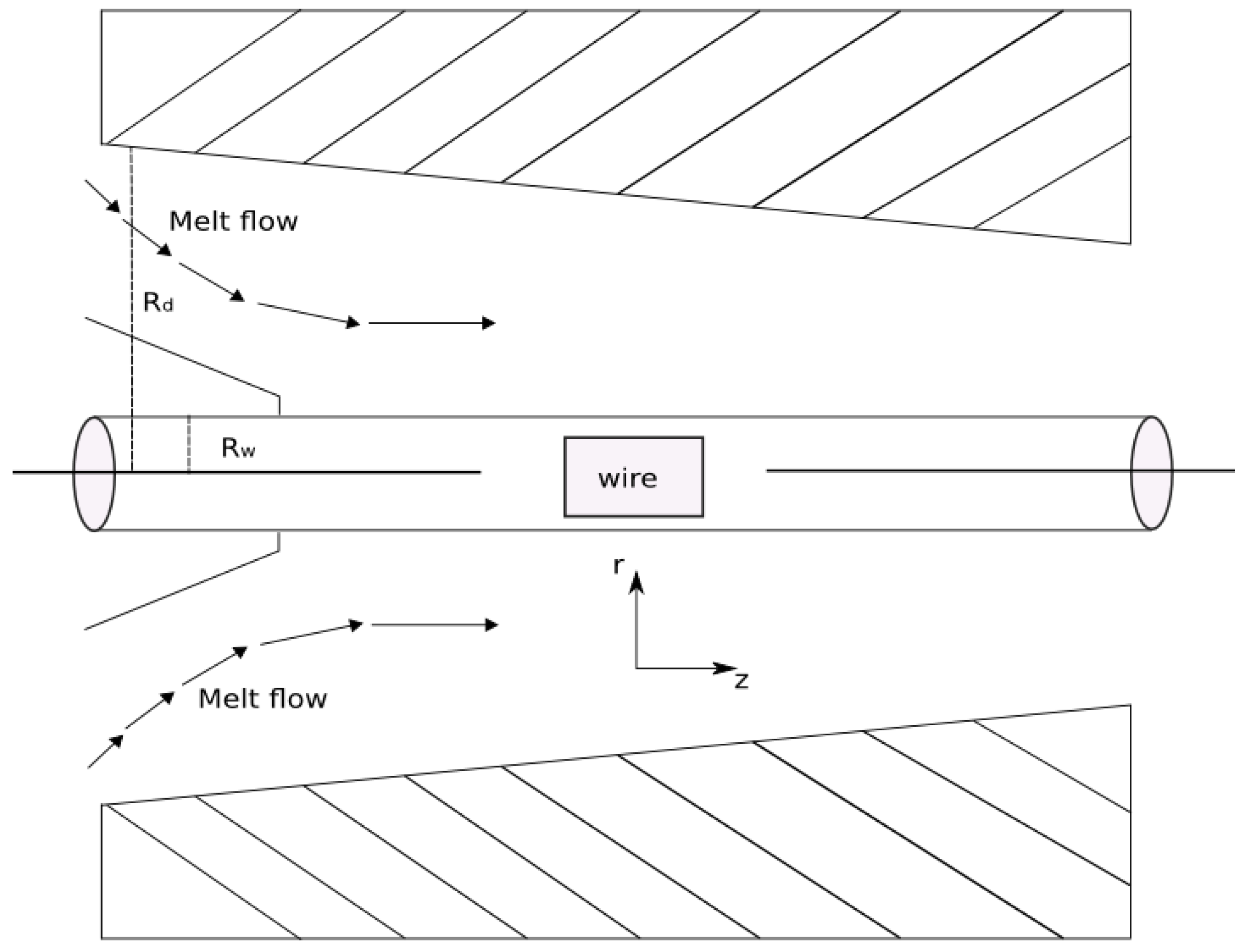
2. Modeling the Problem

The principle of flow geometry is schematically shown in Figure 1. A wire of radius R_w is dragged with velocity v through a pressure-type coating die of length L and radius R_d. The coordinate system is taken at the center of the wire, in which r is taken perpendicular to the flow direction and the z-axis is along the flow. Here Θ_w and Θ_d represents the wire and die temperature, respectively. A constant pressure gradient acts upon the fluid direction and the magnetic field of strength transversely along the axial direction.Due to a small magnetic Reynolds number, the induced magnetic field is negligible, which is also a valid assumption on a laboratory scale.

The design of the coating die is more important because it affects the final product quality. In the current study, a pressurized coating die is considered. The impact of the surrounding temperature is considered for optimal performance.

The coating die is filled with an elastic-viscous fluid. The flow is considered incompressible, laminar, axisymmetric, and steady.

With the assumptions mentioned above, the velocity of the fluid, stress tensor, and temperature field are taken as:

u = [0, 0, w(r)], S = S(r), Θ = Θ(r)

(1)

Subject to the boundary conditions,

w = v at r =R_w and w = 0 at r = R_d

(2)

Θ = Θ_w at r =R_w and Θ = Θ_d at r = R_d

(3)

For an elastic-viscous fluid, the stress tensor is:

$$\mathit{S}+{\mathsf{\gamma }}_1\frac{\mathrm{D}\mathit{S}}{\mathrm{D}t}+\frac{{\mathsf{\gamma }}_3}{2}\left({\mathit{A}}_1\mathit{S}+\mathit{S}{\mathit{A}}_1\right)+\frac{{\mathsf{\gamma }}_5}{2}\left(\mathrm{tr}\mathit{S}\right){\mathit{A}}_1+\frac{{\mathsf{\gamma }}_6}{2}\left(\mathrm{tr}\mathit{S}{\mathit{A}}_1\right)\mathit{I}=\mathsf{\eta }\left({\mathit{A}}_1+{\mathsf{\gamma }}_2\frac{\mathrm{D}{\mathit{A}}_1}{\mathrm{D}t}+{\mathsf{\gamma }}_4{\mathit{A}}_1^2+\frac{{\mathsf{\gamma }}_7}{2}\left(\mathrm{tr}{\mathit{A}}_1^2\right)\mathit{I}\right)$$

(4)

In the above, η is the viscosity of the fluid, D/Dt is the material derivative, S is the extra stress tensor, A₁ is the Rivlin–Ericksen tensor, and γ_i (i = 1–7) are the material constants.

$${\mathit{A}}_1={\mathit{L}}_{\mathrm{T}}=\mathit{L},\mathit{L}=\nabla u$$

(5)

A_n = A_{n − 1}L^T + LA_{n – 1} +DA_{n – 1}/Dt, n = 2, 3,…

(6)

In the above equation,T denotes the transpose of the matrix.

It should be noted that Equation (4) contains several other models: γ₁−γ₇ = 0.

• For the Newtonian fluid model, all γ₁ − γ₇ = 0.
• For the second-grade fluid model, all γ₁ = γ₃ = γ₅ = γ₆ = γ₇ = 0.
• For the Oldroyd-B model, all γ₃ − γ₇ = 0.
• For the Maxwell model, all γ₂ − γ₇ = 0.
• For the Johnson–Segalman model, all γ₅ = γ₆ = γ₇ = 0.
• For the Oldroyd-6model, all γ₆ = γ₇ = 0.

The basic governing equations for incompressible flow are the continuity, momentum, and energy equations given by:

$$\nabla u=0$$

(7)

$$\mathsf{\rho }\frac{\mathrm{D}u}{\mathrm{D}t}=\nabla T+\mathit{J}·\mathit{B}$$

(8)

$$\mathsf{\rho }{c}_p\frac{\mathrm{D}\mathsf{\Theta }}{\mathrm{D}t}=k{\nabla }^2\mathsf{\Theta }+TL$$

(9)

In the above equations u, ρ, T, c_p, D/Dt, k, Θ, are the velocity of the fluid, density of the fluid, shear stress, specific heat, material derivative, thermal conductivity, temperature, and velocity gradient, respectively.

The interaction of current and magnetic field produces a body force J·B as given in Equation (8). The electrostatic force produced due to charge density is negligible and we only consider the applied magnetic field B₀ normal to the flow direction.

In the above frame of reference the body force becomes:

$$\mathit{J}·\mathit{B}=-\sigma {\mathit{B}}_0^{2}w$$

(10)

From Equations (1) and (8)–(10) the velocity and temperature fields become:

$$\begin{array}{l}r\frac{{\mathrm{d}}^{2}w}{\mathrm{d}{r}^2}+\frac{\mathrm{d}w}{\mathrm{d}r}+\left(\mathsf{\alpha }+\mathsf{\beta }\right){\left(\frac{\mathrm{d}w}{\mathrm{d}r}\right)}^3-\mathsf{\beta }r{\left(\frac{\mathrm{d}w}{\mathrm{d}r}\right)}^2\frac{{\mathrm{d}}^{2}w}{\mathrm{d}{r}^2}+\mathsf{\alpha }\mathsf{\beta }r{\left(\frac{\mathrm{d}w}{\mathrm{d}r}\right)}^4\frac{{\mathrm{d}}^{2}w}{\mathrm{d}{r}^2}+3\mathsf{\alpha }r{\left(\frac{\mathrm{d}w}{\mathrm{d}r}\right)}^2\frac{{\mathrm{d}}^{2}w}{\mathrm{d}{r}^2}+\\ \mathsf{\alpha }\mathsf{\beta }{\left(\frac{\mathrm{d}w}{\mathrm{d}r}\right)}^5-\frac{\mathsf{\sigma }{\mathit{B}}_0^2}{\mathsf{\eta }}{\left(1+\mathsf{\beta }{\left(\frac{\mathrm{d}w}{\mathrm{d}r}\right)}^2\right)}^{2}w=0\end{array}$$

(11)

$$k\left(\frac{1}{r}\frac{\mathrm{d}}{\mathrm{d}r}\left(r\frac{\mathrm{d}\mathsf{\Theta }}{\mathrm{d}r}\right)\right)+{\mathit{S}}_{rz}\left(\frac{\mathrm{d}w}{\mathrm{d}r}\right)=0$$

(12)

where

$$\mathsf{\alpha }={\mathsf{\gamma }}_1\left({\mathsf{\gamma }}_4+{\mathsf{\gamma }}_7\right)-\left({\mathsf{\gamma }}_3+{\mathsf{\gamma }}_5\right)\left({\gamma }_4+{\mathsf{\gamma }}_7-{\mathsf{\gamma }}_2\right)-\frac{{\mathsf{\gamma }}_5{\mathsf{\gamma }}_7}{2},\mathsf{\beta }={\mathsf{\gamma }}_1\left({\mathsf{\gamma }}_3+{\mathsf{\gamma }}_6\right)-\left({\mathsf{\gamma }}_3+{\mathsf{\gamma }}_5\right){\mathsf{\gamma }}_1\left({\mathsf{\gamma }}_3+{\mathsf{\gamma }}_6-{\mathsf{\gamma }}_1\right)-\frac{{\mathsf{\gamma }}_5{\mathsf{\gamma }}_6}{2}$$

Introducing the dimensionless parameters:

$$r^{*}=\frac{r}{R_w},w^{*}=\frac{w}{V},{\mathsf{\alpha }}^{*}=\frac{\mathsf{\alpha }{V}^2}{R_w^2},{\mathsf{\beta }}^{*}=\frac{\mathsf{\beta }{V}^2}{R_w^2},M^2=\frac{\mathsf{\sigma }{\mathit{B}}_0^2}{\left(\raisebox{1ex}{$\mathsf{\eta }$}\!\left/ \!\raisebox{-1ex}{$R_w^2$}\right.\right)},\mathsf{\delta }=\frac{R_d}{R_w}>1,\mathsf{\Theta }=\frac{\mathsf{\Theta }-{\mathsf{\Theta }}_w}{{\mathsf{\Theta }}_d-{\mathsf{\Theta }}_w},Br=\frac{\mathsf{\eta }{V}^2}{k({\mathsf{\Theta }}_d-{\mathsf{\Theta }}_w)}$$

(13)

In the above equation α, β are the material parameters, M is the magnetic parameter, δ is the radii ratio, and Br is the Brinkman number.

The system of Equations (2), (3), (11), and (12)in dimensionless form becomes:

$$\begin{array}{c}r\frac{{\mathrm{d}}^{2}w}{\mathrm{d}{r}^2}+\frac{\mathrm{d}w}{\mathrm{d}r}+\left(\mathsf{\alpha }+\mathsf{\beta }\right){\left(\frac{\mathrm{d}w}{\mathrm{d}r}\right)}^3-\mathsf{\beta }r{\left(\frac{\mathrm{d}w}{\mathrm{d}r}\right)}^2\frac{{\mathrm{d}}^{2}w}{\mathrm{d}{r}^2}+\mathsf{\alpha }\mathsf{\beta }r{\left(\frac{\mathrm{d}w}{\mathrm{d}r}\right)}^4\frac{{\mathrm{d}}^{2}w}{\mathrm{d}{r}^2}+3\mathsf{\alpha }r{\left(\frac{\mathrm{d}w}{\mathrm{d}r}\right)}^2\frac{{\mathrm{d}}^{2}w}{\mathrm{d}{r}^2}+\\ \mathsf{\alpha }\mathsf{\beta }{\left(\frac{\mathrm{d}w}{\mathrm{d}r}\right)}^5-M^2\left[1+\mathsf{\beta }{\left(\frac{\mathrm{d}w}{\mathrm{d}r}\right)}^4+2\mathsf{\beta }{\left(\frac{\mathrm{d}w}{dr}\right)}^2\right]=0\end{array}$$

(14)

$$w\left(1\right)=1,w\left(\mathsf{\delta }\right)=0$$

(15)

$$\frac{1}{r}\frac{\mathrm{d}}{\mathrm{d}r}\left(r\frac{\mathrm{d}\mathsf{\Theta }}{\mathrm{d}r}\right)\left(1+\mathsf{\beta }{\left(\frac{\mathrm{d}u}{\mathrm{d}r}\right)}^2\right)+Br\left(1+\mathsf{\alpha }{\left(\frac{\mathrm{d}u}{\mathrm{d}r}\right)}^2\right){\left(\frac{\mathrm{d}u}{\mathrm{d}r}\right)}^2$$

(16)

$$\mathsf{\Theta }\left(1\right)=0,\mathsf{\Theta }\left(\mathsf{\delta }\right)=1$$

(17)

3. Solution of the Modeled Problem

To solve Equations (14)–(17), we apply the Adomian decomposition method [38,39,40,41,42]. The detail of the method is given in the appendix, while the zero and first-order solutions for the velocity field and temperature distributions are:

$$w_0=\frac{-r+\mathsf{\delta }}{-1+\mathsf{\delta }}$$

(18)

$${\mathsf{\Theta }}_0=\frac{-1+r}{-1+\mathsf{\delta }}$$

(19)

$$w_1=\frac{1}{6{\left(-1+\mathsf{\delta }\right)}^5}\left(\begin{array}{l}-M^{2}r+M^2{r}^3+3r\mathsf{\alpha }-3r^2\mathsf{\alpha }+3r\mathsf{\beta }-9M^{2}r\mathsf{\beta }-3r^2\mathsf{\beta }+9M^2{r}^2\mathsf{\beta }-3r\mathsf{\alpha }\mathsf{\beta }+3r^2\mathsf{\alpha }\mathsf{\beta }+\\ M^2\mathsf{\delta }+6M^{2}r\mathsf{\delta }-3M^2{r}^2\mathsf{\delta }-4M^2{r}^3\mathsf{\delta }-3\mathsf{\alpha }\mathsf{\delta }-3r\mathsf{\alpha }\mathsf{\delta }+6r^2\mathsf{\alpha }\mathsf{\delta }-3\mathsf{\beta }\mathsf{\delta }+9M^2\mathsf{\beta }\mathsf{\delta }-\\ 3r\mathsf{\beta }\mathsf{\delta }+6M^{2}r\mathsf{\beta }\mathsf{\delta }+6r^2\mathsf{\beta }\mathsf{\delta }-15M^2{r}^2\mathsf{\beta }\mathsf{\delta }+3\mathsf{\alpha }\mathsf{\beta }\mathsf{\delta }-3r\mathsf{\alpha }\mathsf{\beta }\mathsf{\delta }-6M^2{\mathsf{\delta }}^2-12M^{2}r{\mathsf{\delta }}^2+\\ 12M^2{r}^2{\mathsf{\delta }}^2+6M^2{r}^3{\mathsf{\delta }}^2+6\mathsf{\alpha }{\mathsf{\delta }}^2-3r\mathsf{\alpha }{\mathsf{\delta }}^2-3r^2\mathsf{\alpha }{\mathsf{\delta }}^2+6\mathsf{\beta }{\mathsf{\delta }}^2-15M^2\mathsf{\beta }{\mathsf{\delta }}^2-3r\mathsf{\beta }{\mathsf{\delta }}^2+\\ 9M^{2}r\mathsf{\beta }{\mathsf{\delta }}^2-3r^2\mathsf{\beta }{\mathsf{\delta }}^2+6M^2{r}^2\mathsf{\beta }{\mathsf{\delta }}^2+14M^2{\mathsf{\delta }}^3+8M^{2}r{\mathsf{\delta }}^3-18M^2{r}^2{\mathsf{\delta }}^3-4M^2{r}^3{\mathsf{\delta }}^3\\ -3\mathsf{\alpha }{\mathsf{\delta }}^3+3r\mathsf{\alpha }{\mathsf{\delta }}^3-3\mathsf{\beta }{\mathsf{\delta }}^3+6M^2\mathsf{\beta }{\mathsf{\delta }}^3+3r\mathsf{\beta }{\mathsf{\delta }}^3-6M^{2}r\mathsf{\beta }{\mathsf{\delta }}^3-16M^2{\mathsf{\delta }}^4+3M^{2}r{\mathsf{\delta }}^4+\\ 12M^2{r}^2{\mathsf{\delta }}^4+M^2{r}^3{\mathsf{\delta }}^4+9M^2{\mathsf{\delta }}^5-6M^{2}r{\mathsf{\delta }}^5-3M^2{r}^2{\mathsf{\delta }}^5-2M^2{\mathsf{\delta }}^6+2M^{2}r{\mathsf{\delta }}^6\end{array}\right)$$

(20)

$${\mathsf{\Theta }}_1=\frac{1}{2{\left(-1+\mathsf{\delta }\right)}^4}\left(\begin{array}{l}-rR+r^{2}R-rR\mathsf{\alpha }+r^{2}R\mathsf{\alpha }+R\mathsf{\delta }+rR\mathsf{\delta }-2r^{2}R\mathsf{\delta }+R\mathsf{\alpha }\mathsf{\delta }-rR\mathsf{\alpha }\mathsf{\delta }-2R{\mathsf{\delta }}^2+rR{\mathsf{\delta }}^2\\ +r^{2}R{\mathsf{\delta }}^2+R{\mathsf{\delta }}^3-rR{\mathsf{\delta }}^3-2r\ln r-2r\mathsf{\beta }\ln r+6r\mathsf{\delta }\ln r+2r\mathsf{\beta }\mathsf{\delta }\ln r-\\ 6r{\mathsf{\delta }}^2\ln r+2r{\mathsf{\delta }}^3\ln r+2\mathsf{\delta }\ln \delta -2r\mathsf{\delta }\ln \mathsf{\delta }+2\mathsf{\beta }\mathsf{\delta }\ln \mathsf{\delta }-\\ 2r\mathsf{\beta }\mathsf{\delta }\ln \mathsf{\delta }-4{\mathsf{\delta }}^2\ln \mathsf{\delta }+4r{\mathsf{\delta }}^2\ln \mathsf{\delta }+2{\mathsf{\delta }}^3\ln \mathsf{\delta }-2r{\mathsf{\delta }}^3\ln \mathsf{\delta }\end{array}\right)$$

(21)

The second component is too large, so we only give the graphical representation upto the second-order approximation.

Collecting the results, we have the velocity field and temperature distribution up to a first-order approximation obtained by ADM as follows:

$$w=\frac{-r+\mathsf{\delta }}{-1+\mathsf{\delta }}+\frac{1}{6{\left(-1+\mathsf{\delta }\right)}^5}\left(\begin{array}{l}-M^{2}r+M^2{r}^3+3r\mathsf{\alpha }-3r^2\mathsf{\alpha }+3r\mathsf{\beta }-9M^{2}r\mathsf{\beta }-3r^2\mathsf{\beta }+9M^2{r}^2\mathsf{\beta }-3r\mathsf{\alpha }\mathsf{\beta }+3r^2\mathsf{\alpha }\mathsf{\beta }+\\ M^2\mathsf{\delta }+6M^{2}r\mathsf{\delta }-3M^2{r}^2\mathsf{\delta }-4M^2{r}^3\mathsf{\delta }-3\mathsf{\alpha }\mathsf{\delta }-3r\mathsf{\alpha }\mathsf{\delta }+6r^2\mathsf{\alpha }\mathsf{\delta }-3\mathsf{\beta }\mathsf{\delta }+9M^2\mathsf{\beta }\mathsf{\delta }-\\ 3r\mathsf{\beta }\mathsf{\delta }+6M^{2}r\mathsf{\beta }\mathsf{\delta }+6r^2\mathsf{\beta }\mathsf{\delta }-15M^2{r}^2\mathsf{\beta }\mathsf{\delta }+3\mathsf{\alpha }\mathsf{\beta }\mathsf{\delta }-3r\mathsf{\alpha }\mathsf{\beta }\mathsf{\delta }-6M^2{\mathsf{\delta }}^2-12M^{2}r{\mathsf{\delta }}^2+\\ 12M^2{r}^2{\mathsf{\delta }}^2+6M^2{r}^3{\mathsf{\delta }}^2+6\mathsf{\alpha }{\mathsf{\delta }}^2-3r\mathsf{\alpha }{\mathsf{\delta }}^2-3r^2\mathsf{\alpha }{\mathsf{\delta }}^2+6\mathsf{\beta }{\mathsf{\delta }}^2-15M^2\mathsf{\beta }{\mathsf{\delta }}^2-3r\mathsf{\beta }{\mathsf{\delta }}^2+\\ 9M^{2}r\mathsf{\beta }{\mathsf{\delta }}^2-3r^2\mathsf{\beta }{\mathsf{\delta }}^2+6M^2{r}^2\mathsf{\beta }{\mathsf{\delta }}^2+14M^2{\mathsf{\delta }}^3+8M^{2}r{\mathsf{\delta }}^3-18M^2{r}^2{\mathsf{\delta }}^3-4M^2{r}^3{\mathsf{\delta }}^3\\ -3\mathsf{\alpha }{\mathsf{\delta }}^3+3r\mathsf{\alpha }{\mathsf{\delta }}^3-3\mathsf{\beta }{\mathsf{\delta }}^3+6M^2\mathsf{\beta }{\mathsf{\delta }}^3+3r\mathsf{\beta }{\mathsf{\delta }}^3-6M^{2}r\mathsf{\beta }{\mathsf{\delta }}^3-16M^2{\mathsf{\delta }}^4+3M^{2}r{\mathsf{\delta }}^4+\\ 12M^2{r}^2{\mathsf{\delta }}^4+M^2{r}^3{\mathsf{\delta }}^4+9M^2{\mathsf{\delta }}^5-6M^{2}r{\mathsf{\delta }}^5-3M^2{r}^2{\mathsf{\delta }}^5-2M^2{\mathsf{\delta }}^6+2M^{2}r{\mathsf{\delta }}^6\end{array}\right)$$

(22)

$$\mathsf{\Theta }=\frac{-r+\mathsf{\delta }}{-1+\mathsf{\delta }}+\frac{1}{2{\left(-1+\mathsf{\delta }\right)}^4}\left(\begin{array}{l}-rR+r^{2}R-rR\mathsf{\alpha }+r^{2}R\mathsf{\alpha }+R\mathsf{\delta }+rR\mathsf{\delta }-2r^{2}R\mathsf{\delta }+R\mathsf{\alpha }\mathsf{\delta }-rR\mathsf{\alpha }\mathsf{\delta }-2R{\mathsf{\delta }}^2+rR{\mathsf{\delta }}^2\\ +r^{2}R{\mathsf{\delta }}^2+R{\mathsf{\delta }}^3-rR{\mathsf{\delta }}^3-2r\ln r-2r\mathsf{\beta }\ln r+6r\mathsf{\delta }\ln r+2r\mathsf{\beta }\mathsf{\delta }\ln r-\\ 6r{\mathsf{\delta }}^2\ln r+2r{\mathsf{\delta }}^3\ln r+2\mathsf{\delta }\ln \mathsf{\delta }-2r\mathsf{\delta }\ln \mathsf{\delta }+2\mathsf{\beta }\mathsf{\delta }\ln \mathsf{\delta }-\\ 2r\mathsf{\beta }\mathsf{\delta }\ln \mathsf{\delta }-4{\mathsf{\delta }}^2\ln \mathsf{\delta }+4r{\mathsf{\delta }}^2\ln \mathsf{\delta }+2{\mathsf{\delta }}^3\ln \mathsf{\delta }-2r{\mathsf{\delta }}^3\ln \mathsf{\delta }\end{array}\right)$$

(23)

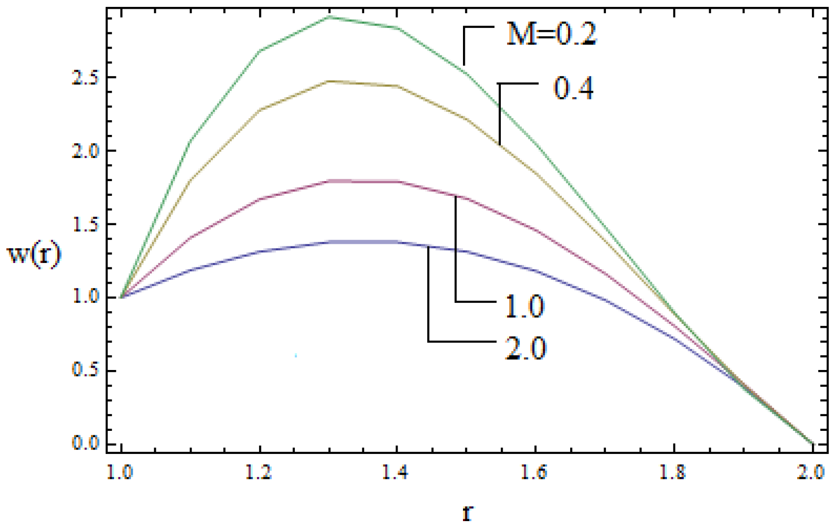
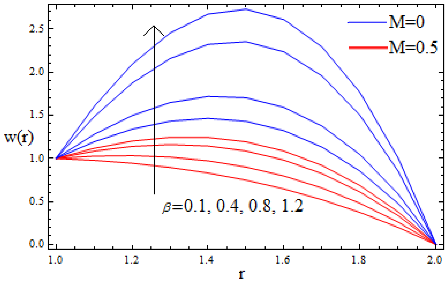
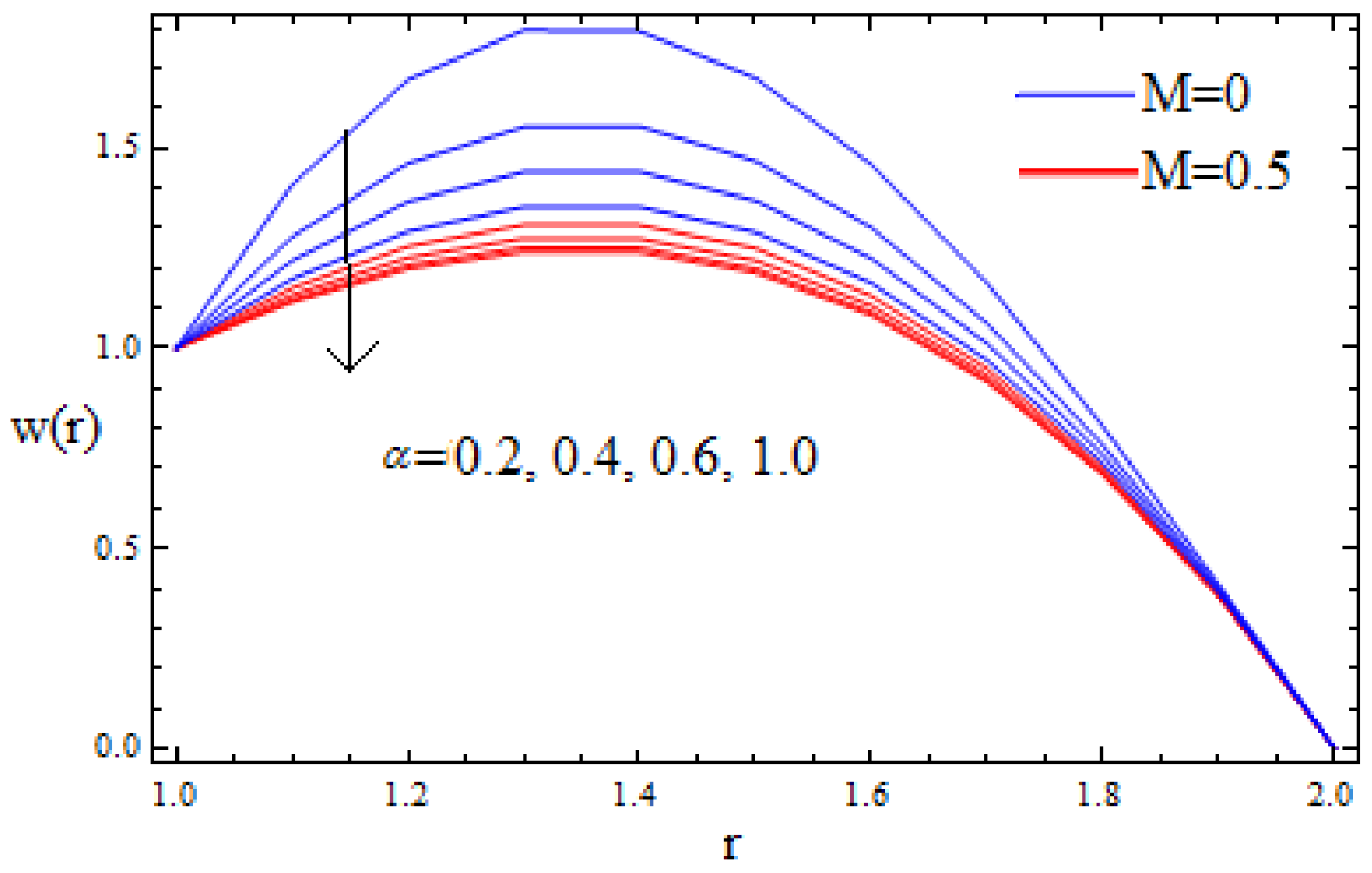
4. Analysis of the Results

The subject of this section is to explore the effect of different emerging parameters such as non-Newtonian parameters α and β magnetic parameter M, and Brinkman number Br on solutions (velocity and temperature profiles), as discussed through several graphs. The convergence of the method and a comparison with the published results are also established in this section.

The convergence of the method is also necessary to check the reliability of the methodology. The convergence of the method is given in

Table B1. Convergence of the method for α = 0.2, β = 0.1, M_i = 0.01, δ = 2.

r	First Order	Second Order
1	0	0
1.1	3.90 × 10−9	2.0 × 10−10
1.2	8.44 × 10−9	3.0 × 10−10
1.3	3.74 × 10−10	9.2 × 10−10
1.4	6.70 × 10−10	1.4 × 10−12
1.5	8.22 × 10−10	1.0 × 10−12
1.6	8.58 × 10−11	2.0 × 10−12
1.7	8.22 × 10−11	1.2 × 10−13
1.8	6.70 × 10−11	7.0 × 10−13
1.9	3.74 × 10−11	2.0 × 10−15
2	8.44 × 10−14	−5.0 × 10−17

,

Table B2. Convergence of the method for α = 0.3, β = 0.2, M_i = 0.1, δ = 2.

r	First Order	Second Order
1	0	0
1.1	7.51 × 10−14	7.93 × 10−16
1.2	2.77 × 10−12	2.21 × 10−14
1.3	1.73 × 10−11	1.11 × 10−13
1.4	5.02 × 10−11	2.46 × 10−13
1.5	9.34 × 10−11	3.12 × 10−13
1.6	1.28 × 10−10	2.43 × 10−13
1.7	1.39 × 10−10	1.15 × 10−13
1.8	1.23 × 10−10	1.40 × 10−14
1.9	–7.50 × 10−11	1.97 × 10−14
2	1.95 × 10−11	2.26 × 10−13

and

Table B3. Convergence of the method for α = 0.4, β = 0.3, M_i= 0.2, δ = 2.

r	First Order	Second Order
1	0	0
1.1	3 × 10−11	2.64 × 10−09
1.2	0	5.03 × 10−09
1.3	–1 × 10−10	6.92 × 10−09
1.4	2 × 10−10	8.14 × 10−09
1.5	1.1 × 10−09	8.55 × 10−09
1.6	4.4 × 10−09	8.14 × 10−09
1.7	1.35 × 10−08	6.92 × 10−08
1.8	3.68 × 10−08	5.03 × 10−10
1.9	9.01 × 10−08	2.64 × 10−11
2	2.027 × 10−07	–9.53 × 10−13

by assigning numerical values to the physical parameters of interest given in Appendix B. From this we conclude that for different values of material parameters we get the convergence of the series solutions. The convergence of method can also be observed from the relative error of OHAM and ADM as given in

Table B4. Numerical comparison of OHAM and ADM when β = 0.2, α = 0.3, δ = 2, M = 0.1, C₁ = −0.001652328, C₂ = −0.00173421, C₃ = 0.0010243621, C₄ = 0.0001825341.

r	OHAM	ADM	Absolute Error
1	1	1	0
1.1	0.001524394	0.001524371	0.0125 × 10−5
1.2	0.001352091	0.001352171	0.004 × 10−5
1.3	0.006210390	0.006230392	0.872 × 10−5
1.4	0.011607241	0.011606221	0.101 × 10−5
1.5	0.010442045	0.010442141	0.712 × 10−5
1.6	0.001520519	0.001522512	0.101 × 10−5
1.7	0.006014981	0.007214980	0.106 × 10−5
1.8	0.000304513	0.000304511	0.103 × 10−5
1.9	0.0000114221	0.0000114221	0.001 × 10−5
2.0	0.00001 × 10−18	0.00013 × 10−19	0.001 × 10−18

. Further,

Table B5. Velocity comparison of the present work with published work [20] when α = 0.2, β = 0.1, M= 0, δ = 2.

r	OHAM	Reference [20]	Absolute Error
1	1	1	0
1.1	0.0011703	0.0011712	0.0000009
1.2	0.0002104	0.0002125	0.0000021
1.3	0.0300722	0.0300710	0.0000012
1.4	0.0216071	0.0216012	0.0000059
1.5	0.0104212	0.0104221	0.0000009
1.6	0.0015412	0.0054533	0.0039121
1.7	0.0071200	0.0071401	0.0000201
1.8	0.0035020	0.0035013	0.0000007
1.9	0.0137500	0.0137521	0.0000021
2	0	0	0

also shows a comparison of present and published work and good agreement is found between the present and published work.

To give a clear overview of the physical problem, Figure 2, Figure 3, Figure 4, Figure 5, Figure 6, Figure 7 and Figure 8 are sketched.

The impact of magnetic parameter M on the velocity profile is displayed in Figure 2. It is observed that the velocity profile decreases via larger M. Physically, by increasing the magnetic parameter the Lorentz force increases. Much resistance is occurring in the motion of the fluid, which reduces the velocity of the fluid. The effect of magnetic parameters Mand the material parameter β on the velocity profile is shown in Figure 3. Larger values of the magnetic parameter increase the Lorentz force, which resists the motion of the fluid and thus the velocity of the fluid is reduced. Figure 4 depicts the impact of α on the velocity profile. It is remarkable to note that parameter α has an accelerated effect on the velocity profiles. Physically increasing α would lead to a reduction in the friction forces and thus the fluid would move with greater velocity.

Thus, it is concluded that the magnetic field and the material parameter helps to slow down the speed of the fluid at any point of the flow domain, while the non-Newtonian parameter β accelerates it. Thus, these parameters can be applied as a controlling device for the required quality. The effect of M on the temperature profile is visualized in Figure 5. From this figure it is clear that the temperature profile increases with increasing values of M. It is also interesting to note that the thermal boundary thickness is an increasing function of magnetic parameter. The effect of Brinkman number Brin the presence and absence of the magnetic parameter on the temperature profile is sketched in Figure 6. It is clear that the temperature profile increases as the Brinkman number increases. This is due to the increase in Lorentz force, which is a resistive force and consequently enhances the temperature profile in the middle of the annular zone.

The effect of material parameter αand the non-Newtonian parameter β on the temperature profiles is shown in Figure 7 and Figure 8 in the presence and absence of a magnetic field, respectively. It is observed that the material parameter αdecreases the temperature profile while the non-Newtonian parameter β accelerates the temperature profile significantly, both in the presence and absence of a magnetic field, at all the points of the melt polymer so as to make the process faster.

5. Conclusions

In this work, the wire coating analysis and the heat transport phenomena corresponding to the steady flow has been studied. The fluid is electrically conducted in the presence of an applied magnetic field. The problem is first modeled and then solved by utilizing ADM. The result is also verified by OHAM. Additionally, the convergence of the method is also verified. The effect of different emerging parameters on the solution is discussed. The material parameter α and the magnetic parameter M have a decelerated effect on the velocity profile. The velocity profile increases with increasing β. The temperature profile increases with increases in the magnetic parameter M, Brinkman number Br, and the material parameter β, and decreases with increasing α. At the end, the present results are also compared with results already available in the literature and a good agreement is found.

References

1. Han, C.D.; Rao, D. The rheology of wire coating extrusion. Polym. Eng. Sci. 1978, 18, 1019–1029. [Google Scholar] [CrossRef]
2. Nayak, M.K. Wire Coating Analysis, 2nd ed.; India Tech: New Delhi, India, 2015. [Google Scholar]
3. Caswell, B.; Tanner, R.J. Wire coating die using finite element methods. Polym. Eng. Sci. 1978, 18, 417–421. [Google Scholar] [CrossRef]
4. Tucker, C.L. Computer Modeling for Polymer Processing; Hanser: Munich, Germany, 1989; pp. 311–317. [Google Scholar]
5. Akter, S.; Hashmi, M.S.J. Analysis of polymer flow in a canonical coating unit: Power law approach. Prog. Org. Coat. 1999, 37, 15–22. [Google Scholar] [CrossRef]
6. Akter, S.; Hashmi, M.S.J. Plasto-hydrodynamic pressure distribution in a tepered geometry wire coating unit. In Sustainable Technology in Manufacturing Industries, Proceedings of the fourteenth Conference of the Irish Manufacturing Committee, 3–5 September 1997; Monaghan, J., Lyons, C.G., Eds.; Trinity College: Dublin, Ireland, 1997; pp. 331–340. [Google Scholar]
7. Siddiqui, A.M.; Haroon, T.; Khan, H. Wire coating extrusion in a pressure-type die in the flow of a third grade fluid. Int. J. Non-Linear Sci. Numeric. Simul. 2009, 10, 247–257. [Google Scholar]
8. Fenner, R.T.; Williams, J.G. Analytical methods of wire coating die design. Trans. Plast. Inst. (London) 1967, 35, 701–706. [Google Scholar]
9. Shah, R.A.; Islam, S.; Siddiqui, A.M.; Haroon, T. Optimal homotopy asymptotic method solution of unsteady second grade fluid in wire coating analysis. J. Ksiam 2011, 15, 201–222. [Google Scholar]
10. Shah, R.A.; Islam, S.; Siddiqui, A.M.; Haroon, T. Exact solution of differential equation arising in the wire coating analysis of an unsteady second grad fluid. Math. Comp. Mod. 2013, 57, 1284–1288. [Google Scholar] [CrossRef]
11. Shah, R.A.; Islam, S.; Ellahi, M.; Haroon, T.; Siddiqui, A.M. Analytical solutions for heat transfer flows of a third Grade fluid in case of post-treatment of wire coating. Int. J. Phys. Sci. 2011, 6, 4213–4223. [Google Scholar]
12. Shah, R.A.; Islam, S.; Siddiqui, A.M.; Haroon, T. Heat transfer by laminar flow of an elastico-viscous fluid in post treatment analysis of wire coating with linearly varying temperature along the coated wire. J. Heat Mass Transfer 2012, 48, 903–914. [Google Scholar] [CrossRef]
13. Mitsoulis, E. Fluid flow and heat transfer in wire coating: A review. Adv. Polym. Technol. 1986, 6, 467–487. [Google Scholar] [CrossRef]
14. Oliveira, P.J.; Pinho, F.T. Analytical solution for fully developed channel and pipe flow of Phan-Thien, Tanner fluids. J. Fluid Mech. 1999, 387, 271–280. [Google Scholar] [CrossRef]
15. Thien, N.P.; Tanner, R.I. A new constitutive equation derived from network theory. J. Non-Newto. Fluid Mech. 1977, 2, 353–365. [Google Scholar] [CrossRef]
16. Kasajima, M.; Ito, K. Post-treatment of polymer extrudate in wire coating. Appl. Polym. Symp. 1973, 20, 221–235. [Google Scholar]
17. Wagner, R.; Mitsoulis, E. Effect of die design on the analysis of wire coating. Adv. Polym. Technol. 1985, 5, 305–325. [Google Scholar] [CrossRef]
18. Bagley, E.B.; Storey, S.H. Wire Wire Prod. 1963, 38, 1104–1122.
19. Pinho, F.T.; Oliveira, P.J. Analysis of forced convection in pipes and channels with simplified Phan-Thien-Tanner fluid. Int. J. Heat Mass Transfer 2000, 43, 2273–2287. [Google Scholar] [CrossRef]
20. Shah, R.A.; Islam, S.; Siddiqui, A.M.; Haroon, T. Wire coating analysis with Oldroyd 8-constant fluid by optimal homotopy asymptotic method. Comput. Math. Appl. 2012, 63, 695–707. [Google Scholar] [CrossRef]
21. Abel, S.; Prasad, K.V.; Mahaboob, A. Buoyancy force and thermal radiation effects in MHD boundary layer viscoelastic fluid flow over continuously moving stretching surface. Int. J. Thermal Sci. 2005, 44, 465–476. [Google Scholar] [CrossRef]
22. Sarpakaya, T. Flow of non-Newtonian fluids in a magnetic field. AIChE J. 1961, 7, 324–328. [Google Scholar] [CrossRef]
23. Abel, M.S.; Shinde, J.V.; Shinde, J.N. The effects of MHD flow and heat transfer for the UCM fluid over a stretching surface in presence of thermal radiation. Adv. Math. Phys. 2012, 702681. [Google Scholar] [CrossRef]
24. Chen, V.C. On the analytical solution of MHD flow and heat transfer for two types of viscoelastic fluid over a stretching sheet with energy dissipation, internal heat source and thermal radiation. Int. J. Heat Mass Transfer 2010, 19, 4264–4273. [Google Scholar] [CrossRef]
25. Akbar, N.S.; Ebaid, A.; Khan, Z.H. Numerical analysis of magnetic field effects on Eyring-Powell fluid flow towards a stretching sheet. J. Magn. Magn. Mater. 2015, 382, 355–358. [Google Scholar] [CrossRef]
26. Mabood, F.; Khan, W.A.; Ismail, A.I.M. MHD boundary layer flow and heat transfer of nanofluids over a nonlinear stretching sheet. J. Magn. Magn. Mater. 2015, 374, 569–576. [Google Scholar] [CrossRef]
27. Singh, V.; Agarwal, S. MHD flow and heat transfer for Maxwell fluid over an exponentially stretching sheet with variable thermal conductivity in porous medium. Int. J. Non-Linear Mech. 2005, 40, 1220–1228. [Google Scholar] [CrossRef]
28. Hayat, T.; Sajid, M. Homotopy analysis of MHD boundary layer flow of an upper-convected Maxwell fluid. Int. J. Eng. Sci. 2007, 45, 393–401. [Google Scholar] [CrossRef]
29. Wang, Y.; Hayat, T. Fluctuating flow of a Maxwell fluid past a porous plate with variable suction. Nonlinear Anal. Real World Appl. 2008, 9, 1269–1282. [Google Scholar] [CrossRef]
30. Rashidi, S.; Dehghan, M. Study of stream wise transverse magnetic fluid flow with heat transfer around an obstacle embedded in a porous medium. J. Magn. Magn. Mater. 2015, 378, 128–137. [Google Scholar] [CrossRef]
31. Ellahi, R.; Rahman, S.U.; Nadeem, S.; Vafai, K. The blood flow of Prandtl fluid through a tapered stenosed arteries in permeable walls with magnetic field. Commun. Theor. Phys. 2015, 63, 353–358. [Google Scholar] [CrossRef]
32. Kandelousi, M.S.; Ellahi, R. Simulation of ferrofluid flow for magnetic drug targeting using the lattice Boltzmann method. Zeitschrift für Naturforschung A 2015, 70, 115–124. [Google Scholar] [CrossRef]
33. Hayat, T.; Khan, M.; Asghar, S. Homotopy analysis of MHD flows of an Oldroyd 8-contant fluid. Acta Mech. 2004, 168, 213–232. [Google Scholar] [CrossRef]
34. Ellahi, R.; Hayat, T.; Mahmood, F.M.; Zeeshan, A. Exact solutions for flow of an oldroyd 8-contant fluid with non-linear slip conditions. Commun. Non-Linear Scie. Numer. Simul. 2009, 15, 322–330. [Google Scholar] [CrossRef]
35. Bari, S. Flow of an Oldroyd 8-constant fluid in a convergent channel. Acta Mech. 2001, 148, 117–127. [Google Scholar] [CrossRef]
36. Ellahi, R.; Hayat, T.; Javed, T.; Asghar, S. On the analytic solution of non-linear flow problem involving Oldroyd 8-constant fluid. Math. Comp. Model. 2008, 48, 1191–1200. [Google Scholar] [CrossRef]
37. Zhu, T.; Ye, W. Theoretical and Numerical Studies of Noncontinuum Gas-Phase Heat Conduction in Micro/Nano Devices. Numer. Heat Transfer Part B 2010, 57, 203–226. [Google Scholar] [CrossRef]
38. Liu, H.; Xu, K.; Zhu, T.; Ye, W. Multiple temperature kinetic model and its applications to micro-scale gas flows. Comp. Fluids 2012, 67, 115–122. [Google Scholar] [CrossRef]
39. Adomian, G.A. Review of the decomposition method and some recent results for non-linear equations. Math Comput. Model. 1992, 13, 287–299. [Google Scholar]
40. Wazwaz, A.M. Adomiandecomposition method for a reliable treatment of the Bratu-type equations. Appl. Math. Comput. 2005, 166, 652–663. [Google Scholar]
41. Wazwaz, A.M. Adomian decomposition method for a reliable treatment of the Emden–Fowler equation. Appl. Math. Comput. 2005, 161, 543–560. [Google Scholar] [CrossRef]
42. Zeeshan; Islam, S.; Shah, R.A.; Khan, I.; Gul, T.; Gaskel, P. Double-layer Optical Fiber Coating Analysis by Withdrawal from a Bath of Oldroyd 8-constant Fluid. J. Appl. Environ. Biol. Sci. 2015, 5, 36–51. [Google Scholar]
43. Gul, T.; Shah, R.A.; Islam, S.; Arif, M. MHD thin film flows of a third grade fluid on a vertical belt with slip boundary conditions. J. Appl. Math. 2013, 707286. [Google Scholar]
44. Marinca, V.; Herisanu, N.; Nemes, I. Optimal homotopy asymptotic method with application to thin film flow. Cent. Eur. J. Phys. 2008, 6, 648–653. [Google Scholar] [CrossRef]
45. Marinca, V.; Herişanu, N. Application of Optimal Homotopy Asymptotic Method for solving non-linear equations arising in heat transfer. Int. Commun. Heat Mass Transfer 2008, 35, 710–715. [Google Scholar] [CrossRef]
46. Marinca, V.; Herişanu, N.; Bota, C.; Marinca, B. An Optimal HomotopyAsymptotic Method applied to the steady flow of a fourth grade fluid past a porous plate. Appl. Math. Lett. 2009, 22, 245–251. [Google Scholar] [CrossRef]
Figure 1. Pressure-type coating die for wire coating analysis.
Coatings 07 00015 g001
Figure 2. Velocity profile for various values of M when α = 0.3, β = 0.2, δ = 2.
Coatings 07 00015 g002
Figure 3. Velocity profile for various values of β when α = 0.3, β = 2, M = 0.1.
Coatings 07 00015 g003
Figure 4. Velocity profile for various values of α when β = 0.3, δ = 2, M = 0.1.
Coatings 07 00015 g004
Figure 5. Temperature profile for various of M when α = 0.3, β = 0.2, δ = 2.
Coatings 07 00015 g005
Figure 6. Temperature profile for various of Br when α = 0.4, β = 0.2, M = 0.2, δ = 2.
Coatings 07 00015 g006
Figure 7. Temperature profile for various of α when β = 0.2, M = 0.2, δ = 2.
Coatings 07 00015 g007
Figure 8. Temperature profile for various of β when α = 0.3, M = 0.2, δ = 2.
Coatings 07 00015 g008