Abstract
In recent years, detecting anomalies in real-world computer networks has become a more and more challenging task due to the steady increase of high-volume, high-speed and high-dimensional streaming data, for which ground truth information is not available. Efficient detection schemes applied on networked embedded devices need to be fast and memory-constrained, and must be capable of dealing with concept drifts when they occur. Different approaches for unsupervised online outlier detection have been designed to deal with these circumstances in order to reliably detect malicious activity. In this paper, we introduce a novel framework called PCB-iForest, which generalized, is able to incorporate any ensemble-based online OD method to function on streaming data. Carefully engineered requirements are compared to the most popular state-of-the-art online methods with an in-depth focus on variants based on the widely accepted isolation forest algorithm, thereby highlighting the lack of a flexible and efficient solution which is satisfied by PCB-iForest. Therefore, we integrate two variants into PCB-iForest—an isolation forest improvement called extended isolation forest and a classic isolation forest variant equipped with the functionality to score features according to their contributions to a sample’s anomalousness. Extensive experiments were performed on 23 different multi-disciplinary and security-related real-world datasets in order to comprehensively evaluate the performance of our implementation compared with off-the-shelf methods. The discussion of results, including , score and averaged execution time metric, shows that PCB-iForest clearly outperformed the state-of-the-art competitors in 61% of cases and even achieved more promising results in terms of the tradeoff between classification and computational costs.
1. Introduction
As the diversity and number of interconnected embedded devices steadily grow, energized by various trends, such as IoT, network monitoring, including traffic-based intrusion detection, will play a crucial role in future systems. Although being a fundamental part of computer network security, intrusion detection systems (IDSs) still face major challenges [1,2,3], e.g., the inability to handle massive amounts of throughput and process data in almost real-time due to inherent resource limitations. The permeating application of machine learning (ML) has favored the detection of novel sophisticated network-based attacks changing their behavior dynamically and autonomously. In particular, unsupervised outlier detection (OD) algorithms can help uncover policy violations or noisy instances as indicators of attacks by observing deviations in high-dimensional and high-volume data without requiring a priori knowledge. However, the ubiquity of massive continuously generated data streams across multiple domains in different applications poses an enormous challenge to state-of-the-art, offline, unsupervised OD algorithms that process data as a batches. Data streams in real-world applications are encountering evolving data which are enormous in number, potentially infinite; data are continuously streaming from many places in almost real-time. Therefore, efficient and optimized schemes, in terms of processing time and memory usage, in intelligently designed IDSs are required. These should be able to process the time-varying and rapid data streams one-pass at a time, while only a limited number of data records can be accessed. Furthermore, legitimate changes in data can occur over time, called concept drift, which require updates to a model in order to counteract less accurate predictions as time passes.
Recently, many OD solutions have been developed that are able to compute anomaly scores while dealing with data streams. Data streams can be subdivided into streaming data (SD) and streaming features. In this work, we do not focus on the latter case in which the amount of features changes over time. Furthermore, we do not focus on SD in the context of time-series data, as it is the object of many other research papers, such as [4,5]. In this paper, we first highlight the most popular OD solutions for SD with an in-depth view of promising online variants of one of the most widely accepted (offline) OD algorithms called isolation forest (iForest) [6]. Moreover, substantial requirements are derived to compare the existing state-of-the-art solutions. As the main contribution of this article, we propose the so-called Performance Counter-Based iForest, denoted as PCB-iForest, a generic and flexible framework that is able to incorporate almost any ensemble-based OD algorithm. However, in this work, we focus on two iForest-based variants, an improvement of classical iForest applied in a streaming setting and a variant of classical iForest able to score features according to their contributions to a data record’s anomalousness in a completely unsupervised way. PCB-iForest is able to deal with concept drifts with a dedicated drift detection method, as we take advantage of the recently proposed NDKSWIN algorithm [7]. Our solution is hyperparameter-sparse, meaning that one does not have to deal with complex hyperparameter settings, which often demands a priori knowledge. In extensive experiments involving various multi-disciplinary but also security-related datasets with different characteristics, we show that the proposed PCB-iForest variants outperform off-the-shelf, state-of-the-art competitors in the majority of cases. This work offers the following contributions and mainly differs from others presented in Section 2 in said ways:
- Carefully engineered and specified requirements for an agile, future-oriented, online OD algorithm design are derived, which are compared with state-of-the-art solutions, thereby pointing out the need for a more flexible solution which, consequently, is presented in this article.
- Contrary to other adaptions of iForest for SD, a flexible framework called PCB-iForest is proposed that "wraps around" any iForest-based learner (it might even be generalized to other ensemble-based approaches) and regularly updates the model in cases of concept drift by only discarding outdated ensemble components.
- Two iForest-centric base learners are integrated into PCB-iForest providing (i) the first application of the improved iForest solution—extended isolation forest—on SD denoted as PCB-iForestEIF, and (ii) online feature importance scoring by utilizing a recent iForest-based feature selection method for static data—isolation-based feature selection (IBFS)—in our online proposal, denoted as PCB-iForestIBFS.
- Extensive evaluations were conducted for PCB-iForest and off-the-shelf online OD algorithms on numerous, multi-disciplinary datasets with diversity in the numbers of dimensions and instances which no other iForest-based competitor for SD has dealt with yet.
The remainder of this work is organized as follows—Section 2 first provides relevant background for the reader for unsupervised OD on SD and provides related work with the most popular state-of-the-art solutions, especially existing iForest adaptions for SD. Substantial requirements for online OD algorithms are derived in Section 3 and compared with the related work. In Section 4, details on the conceptualization and operating principle of PCB-iForest can be found. It is able to satisfy all requirements stated in Section 3. In Section 5, the test environment is presented, and details on the extensive evaluation are presented together with the discussion of results (Section 6), which reveals the superiority of PCB-iForest among the state-of-the-art by most the measurements. The conclusions are drawn in Section 7, alongside glances at future work.
2. Related Work
Outlier detection, also referred to as anomaly or novelty detection, is an important issue for many real-world application domains, especially detecting indicators of malicious activity in computer networks. Outlier detection identifies atypical patterns or observations that significantly deviate from the norm based on some measure by assuming that (i) the majority of data are normal and there is only a small portion of outliers (imbalance); (ii) outliers are statistically different from the normal data (distinction) and (iii) they do not occur frequently (rarity). Numerous techniques have been introduced for OD, such as statistical, distance, clustering or density-based ones [8]. An OD algorithm assigns a class label or a score value , describing the strengths of anomalousness, for each data object in X. This divides X into a set of outliers and inliers (). In the streaming setting, is a continuous transmission of data records which arrive sequentially at each time step t. The count of features is denoted as d (dimension) and the -th d-dimensional, most recent incoming data instance at time t.
To concentrate on supervised or semi-supervised learning, widely accepted online anomaly detection algorithms such as Hoeffding trees [9] and online random forests [10] achieve good accuracy and robustness in data streams [11]. However, the main focus of this work lies on unsupervised approaches, since the amount of unlabeled data with missing ground truth generated across many scientific disciplines, especially intrusion detection, has steadily increased. In recent years, many methods have been proposed for unsupervised online OD, such as [12,13,14], but only a few of them apart from iForest, namely, HS-Trees [15], RS-Hash [16] and Loda [17] have been shown to outperform numerous standard detectors and hence are considered the state-of-the-art [18,19]. Since xStream proposed in [18] is as competitive as those detectors, particularly effective in high-dimensions and revolutionized online OD algorithms by being able to deal with streaming features, we count it on the list of the state-of-the-art.
RS-Hash samples axis-parallel, subspace grid regions of varying size and dimensionality to score data points by utilizing the concept of randomized hashing. Its adaption, RS-Stream, is able to operate on SD by computing the log-likelihood density model using time-decayed scores. Thus, compared to other work that applies sliding windows, for example, it uses continuous counting where points are down-weighted by their up-to-dateness. Compared to RS-Hash, the streaming variant requires greater sophistication in the hash-table design and maintenance, although the overall approach is quite similar [20].
Loda, a lightweight online detector of anomalies, is an ensemble approach consisting of a collection of h one-dimensional histograms; each histogram approximates the probability density of the input data projected onto a single projection vector. Projection vectors diversify individual histograms, which is a necessary condition to improve the performance of individual classifiers in high-dimensional data. The features used must only be of approximately the same order of magnitude, which is an improvement over other methods, such as HS-Trees. Loda’s output on a sample x is the averaged logarithm of the probabilities estimated on a single projection vector. It is especially useful in domains where large numbers of samples have to be processed, because its design facilitates very good balance between accuracy and complexity. The algorithm exists in different variants for batch and online learning. For online processing, a subdivision can be made. Similarly to HS-Trees, two alternating histograms can be used in Loda, denoted as LodaTwo Hist., where the older set of histograms is used for classification and the newer one is built in the current window. If the new set is built, it replaces the currently used histogram set. A floating window approach, LodaCont., denotes an implementation of continuously updated histograms based on [21].
xStream is able to deal with data streams that are characterized by SD in terms of instances (rows), and evolving, newly-emerging features can be processed while xStream remains constant in space and time. Due to a fixed number of bins for the one-dimensional histograms, growing feature space cannot be handled by Loda. The authors of xStream overcame this limitation by so-called half-space chains where the data, independently of streaming features, are projected via sparse random projection into recursively constructed partitions with splits into small, flexible bins. This density-based ensemble handles non-stationarity, similarly to HS-Trees and LodaTwo Hist., by a pair of alternating windows.
The random forest is one of the most successful models used in classification and is known to outperform the majority of classifiers in a variety of problem domains [20,22]. Due to their intuitive similarity, iForest is an unsupervised approach that has been established as one of the most important methods in the field of OD. Much work has been done to improve iForest, e.g., [23,24], and to adapt it to other application scenarios, such as feature selection [25]. Even if it was initially not designed to work as an online algorithm, over the last few years, manifold variants of online algorithms have been proposed that are either based on iForest’s concept or adapt it to operate in a streaming fashion.
HS-Trees, a collection of random half-space-trees, is based on a similar tree ensemble concept as iForest. HS-Trees has a different node splitting criterion and calculates the anomaly scores based on the sample counts and densities of the nodes. Furthermore, the trees have a fixed depth (height), whereas iForest uses adaptive depths with smaller subspaces. For SD with concept drifts, HS-Trees utilizes two windows (batches) of equal size, and as in the learning of HS-Trees in the current window, the HS-Trees trained in the previous one replace the old.
One of the first approaches adopting iForest for SD was iForestASD proposed in [26]. It utilizes a sliding window with a fixed length to sample data with which the ensemble of trees is built. Based on a predefined threshold value, changes within the window can be detected. In the case of an occurring concept drift, this leads to a re-training of the whole ensemble based on the information of the current sliding window content. The authors themselves proposed significant improvements for future work. For instance, that the predefined threshold relying on a priori knowledge should be replaced alongside partial re-training of only some trees was suggested, rather than discarding the complete model. A detailed description of the differences between HS-Trees and iForestASD can be found in [7].
Recently, iForestASD has been implemented in an open source ML framework for data streams scikit-multiflow [27] and improved in [7] to better handle concept drifts by extending it using various drift detection methods. Therefore, the authors extended ADWIN [28] and KSWIN [29] drift detectors and denoted them SADWIN/PADWIN and NDKSWIN. Their OD solutions in this article are denoted as IFA(S/P)ADWIN and IFANDKSWIN. However, some major disadvantages of their proposals, such as partially updating the model rather than discarding the complete forest, have still been present in subsequent work.
More recently, the work of [30] improved LSHiForest, a classifier based on iForest to handle high-dimensional data while detecting special anomalies, e.g., axis-parallel ones, to handle SD and produce time-efficient results when processing large, high-dimensional datasets. Their improvement, denoted as LSHiForestStream in this article, consists of a combination of streaming pre-processing based on dimensionality reduction with principal component analysis (PCA) and a weighted Page–Hinckley test to find suspicious data points. Furthermore, locality sensitive hashing is applied that hashes similar input items into the same branches with high probability, and dynamic iForest is applied with efficient updating strategies. Thus, rather than exchanging the whole model as with iForestASD, this approach repeatedly checks if new suspicious data points exist and updates them in the tree structure.
Another hybrid method called iMondrian forest, denoted as iMForest, was proposed in [31]. Mondrian forest is a method based on the Mondrian processes for classification and regression on SD. The authors embedded the concept of isolation from iForest by using the depth of a node within a tree and the data structure used in Mondrian forest to operate for OD on SD.
The concept of growing random trees or GR-Trees was proposed in [11], which is also capable of partially updating the ensemble of random binary trees. The GR-Trees approach is quite like the iForest with respect to the training process, as is the approach for anomaly score assignment to the data instances. In an initial stage using the first sliding window content, the ensemble is built without explicit training data. Incremental learning is achieved by combining an update trigger deciding when to update the ensemble. Online tree growth and mass weighting ensure that the model can be adapted in time and is able to handle concept drifts.
Referring to Section 4, most related to our PCB-iForest approach—in order to only partially update the ensemble-based model rather than completely discarding it (as present in iForestASD and IFA variants)—are the solutions presented within LSHiForestStream, iMForest and GR-Trees. Both LSHiForestStream and iMForest do not fulfill the requirement of algorithm agility because of being tailored to dedicated data structures for online learning and classification, rather complexly in the case of LSHiForest. Since LSHiForestStream is designed to deal with multi-dimensional multi-stream data, it is seemingly more computationally intensive than multi-dimensional, single-stream solutions, and considering the inclusion of k-means clustering for anomaly detection in online mode, the same applies for iMForest. GR-Trees is similar to iForest in its training and classification process, and in its framework for SD. During online detection of an initially created ensemble, the classified normal instances are stored in a buffer and are used for the streaming updates, leading to tree growth and updating the trees in the ensemble. The trees are discarded based on the mass weights of the results evaluated by each tree for the sliding window. The tree online growth and mass weighting mechanisms ensure that the detection model can be adjusted in time as the data distribution changes to avoid misjudgments caused by concept drift. Apart from the sliding window, our approach does not need an additional buffer which preserves memory. Additional hyperparameters, such as update rate and discard rate, rather than the ensemble size and subsample size, could require some adjustments to suit the actual needs to obtain better results. Furthermore, apart from the replacement of discarded trees with trees obtained from a building window, existing trees are updated based on an update window. Both mechanisms use the buffered normal instances, which could pose a slight performance issue, as stated in [6]; refer to the section “Training using normal instances only”.
3. Requirement Specification and Validation
In this section, we specify the requirements OD algorithms for SD have to satisfy to be applied in real-world, future-oriented scenarios. Additionally, some requirements are added that help with a holistic incident handling process—for example, providing functionality to assist with identifying the root causes of incidents rooted in outliers. We structure the requirements into operation, data, performance and functionality-related ones.
As already pointed out in the introduction, the missing ground truth values in evolving (theoretically infinite) data that require real or almost near real-time processing, taking the evolution and speed of data feeding into account, demands unsupervised methods, leading to the requirement we will denote as (R-OD01). In addition, those must be capable of dealing with SD (R-OD02). Both requirements are categorized into the operation-related ones.
We can see additional requirements, as follows, that shall play a major role in future systems. Another operation-related requirement is that the settings of hyperparameters should be of low complexity, and in particular, no information of ground truth should be mandatory for the settings, or even better, no hyperparameters should be set at all (R-OD03). This requirement is important since, nowadays, domain experts are expected to have a high level of multi-disciplinary expertise from data science, e.g., extensive knowledge in statistics, in order to properly set up a machine learning pipeline. Even if recent developments in the field of automated machine learning [32] have tried to aid domain experts, they require extensive offline supervised training and testing for each hyperparameter value, and thus do not operate in the unsupervised online cases. Hence, aiding the domain experts by not burdening them with setting parameters seems important for manageable systems. Furthermore, the time-varying nature of SD, especially in highly dynamic networks, is subject to the phenomenon called concept drift. This means the data stream distribution changes over time. With the different types of concept drifts (sudden, gradual, incremental, recurring and blips) [33], algorithms must be able to efficiently adapt to these changes and continuously re-train or update their models (R-OD04) to prevent being outdated, which would lead to performance degradation. Dedicated drift detection methods might come to the rescue for OD algorithms to deal with data’s varying nature.
From a data-related perspective, in the field of network-based OD, data flow from a single source (single-view) and do not necessarily have to be normalized (R-OD05)—e.g., as a raw network interface, as statistics from network switching elements or in the form of log-files from devices. Features can be defined in advance by an expert since incorporating domain knowledge can help select relevant features to improve learning performance greatly. Thus, the cardinality of the feature set (meaning the number of dimensions) is fixed (R-OD06), thereby not demanding algorithms that are able to deal with streaming features. For network-based features, one may distinguish between basic features (derived from raw packet headers (meta data) without inspecting the payload, e.g., ports, and MAC or IP addresses), content-based features (derived from payload assessment having domain knowledge, e.g., protocol specification), time-based features (temporal features obtained from, e.g., message transmission frequency and sliding window approaches) and connection-based features (obtained from a historical window incorporating the last n packets) [34]. However, with the technological advancements and the increasing of potential features, the algorithms must efficiently operate on high-dimensional and high-volumes of data (R-OD07) and must cope with missing variables that might occur due to unreliable data sources (R-OD08).
Performance-related requirements can be subdivided into computational and classification performance requirements. The former demands lightweight algorithms (R-OD09), in terms of time and space complexity, for both model-updating and classification, to be implementable in embedded software. SD is potentially infinite, and algorithms must temporarily store as little data as possible and process the data as fast as possible due to the time constraint of observing incoming data in a limited amount of time. The classification performance needs to be sufficiently good (R-OD10), i.e., producing decent area under the curve (), in which is the receiver operating characteristic, or score metric, in order to detect malicious activity in a reliable way. It should be noted that stream methods, compared to their batch competitors, typically perform worse in terms of classification. However, under the assumption of applying a subsequent root cause analysis, we strongly support the justification in [27] that when considering critical SD applications, an efficient method, even with less accuracy, is preferred.
Functionality-related requirements can be subdivided as follows. One still unresolved issue for IDS is the lack of finding the actual root cause of incidents. Instead of yielding simple binary values (normal or abnormal), requirement (R-OD11) demands algorithms that provide outlier score values. Those carry more information and could help a subsequent root cause analysis, for instance, by dealing with false negatives. In addition, the importance of features can play an important role, thereby demanding functionality to score or rank features according to their outlier score contributions (R-OD12), and so providing information about which feature (mainly) caused the outlier. Reducing the data’s dimensionality can help deal with the curse of dimensionality, referring to the phenomenon that data becomes sparser in high-dimensional space and can still be represented accurately with less dimensions. This adversely affects both the storage requirements and computational cost of the algorithms. Reduction by methods such as PCA maps higher-order matrices into ones with lower dimensions with a certain probability. However, the physical meaning of the features is no longer retained by this projection and impedes root cause analysis (feature interpretability). Feature selection methods reduce the dimensions by only selecting the most relevant features, and hence, preserve their physical meanings. Applying feature selection on SD would possibly lead to changing top-performing-features as time passes and thus demand for OD algorithms that are capable of changing feature sets during runtime (R-OD13). Considering the multitude of recent work that is tailored to attack machine learning, e.g., [35,36], we can see, similarly to cryptographic agility, the flexibility to exchange the actual algorithm as a forward-looking requirement (R-OD14) in the case where the currently used algorithm (poisoning) or its model (evasion) gets compromised. More likely it is the former, since an evasion of the model seems, due to the continuous updating, more irrelevant.
Over the past few years, much attention has been paid to establishing OD algorithms for SD in the field of network security, and is increasingly facing trends of massive amounts of data generated with high velocity and afflicted with the phenomenon of concept drift. Many existing works have tried to improve the algorithm settings in terms of performance-related requirements by competing on the same (often outdated) benchmark dataset. For real-world applications, in which most of the algorithms might perform insufficiently, we expect that designing algorithms and finding a tradeoff between the stated requirements is more crucial. Thus, assuming the application of a subsequent root cause analysis enabled by, e.g., (R-OD12), certain numbers of false positives and false negatives are acceptable when referring to (R-OD10). In particular, considering critical application domains, it might be preferred to quickly and efficiently detect outliers, even with less accuracy. Table 1 validates state-of-the-art algorithms presented in Section 2 using the specified requirements. It can clearly be seen that none of the existing methods have good results across the majority of requirements.

Table 1.
Comparison of existing OD work for SD from Section 2 with the requirements specified (✓ and ✗ denote the requirement is either fulfilled or not, respectively; ⌀ denotes missing information to analyze the respective requirement; (+/++/+++) denotes—as objectively as possible—how well the requirement is fulfilled).
4. Generic PCB-iForest Framework
In this section we focus on the design of an intelligent OD solution that is able to satisfy all of the aforementioned requirements. Thus, we carefully reviewed related work and combined the merits of the most promising approaches while alleviating their shortcomings. Our focus lies on the iForest-based approaches, since iForest is (i) a state-of-the-art algorithm for OD, (ii) widely used by the community, (iii) efficient in terms of computational and classification performance and (iv) can easily be adapted for the SD application [7]. The wide acceptance in research is reflected in numerous improvements and extensions—for instance, extended isolation forest (EIF) [23], functional isolation forest [24], entropy iForest [37], LSHiForest [38] and SA-iForest [39]—for different application domains or focusing on special problems, such as dealing with categorical and missing data [40]. However, those adaptions are mainly tailored for static datasets rather than the application on SD. Thus, our aim was to provide a framework that is able to exchange the iForest-based classifier in cases of compromising data or if the application domain, with its specific task, demands another base learner. Moreover, the framework can be generalized to basically incorporate any ensemble-based algorithm consisting of a set of components such as trees. The workflow of our so-called Performance Counter-Based iForest framework, denoted as PCB-iForest, is shown in Figure 1.
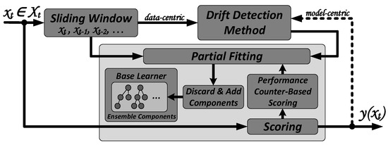
Figure 1.
The workflow of PCB-iForest’s incremental learning framework.
Data instance (data point) with dimensions d of the data stream will be captured as the latest instance at each time step t in the count-based sliding window W and in parallel will be evaluated in the Scoring module, which provides an outlier score y for each . The sliding window is composed of the latest w instances such that . A dedicated drift detection method is applied that triggers the partial fitting process to discard and add components, denoted as C, of the ensemble E. The core of PCB-iForest is the Performance Counter-Based Scoring module, which is able to identify well and badly performing components of an ensemble. Partial fitting will then discard only the poorly-performing data and replaces them with newly created ones from the most recent instances contained in the sliding window. In the following, we provide more details on the main parts of our framework.
4.1. Drift Detection Method
Detecting changes in multi-dimensional SD is a challenging problem, especially when considering scaling with the number of dimensions. A sometimes applied solution is to reduce the number of dimensions by either performing PCA (cf. LSHiForestStream) or random projections. Furthermore, one might even reduce the number to one (or more) uni-dimensional statistics and apply a well-known drift detection method, such as DDM [41] or ADWIN [28,42]. For IFA(S/P)ADWIN, drift detection will be performed on the one-dimensional statistic of either the binary prediction value (PADWIN) or the actual score value (SADWIN). Reduction is achieved by the learning model. Thus, it is referred to as a model-centric approach. However, generic approaches, such as [43,44], exist that deal with multi-dimensional changes performed specifically on the SD, referred to as data-centric.
We can see that model-centric approaches (indicated by the dotted line in Figure 1) might be prone to a phenomenon called positive feedback. This means that drift detection causing partial fitting will be negatively influenced by the actual classification results in such a way that the ensemble results tend to be the same by discarding “badly” performing components from the model point of view. Positive feedback is also present within iForestASD, since drift detection depends on the anomaly rate computed by the model’s scoring results. Furthermore, iForestASD’s anomaly rate is dependent on a priori knowledge, which is hardly feasible in real-world applications. Therefore, we recommend the usage of data-centric solutions, which are unbiased of the applied model only relying on the SD characteristics. Since NDKSWIN in [7] has, as of now, proven to be a reliable drift detection method, we are applying it to PCB-iForest, but our approach is open to any data-centric or model-centric solution. NDKSWIN adapts a relatively new one-dimensional method called KSWIN [29] based on the Kolmogorov–Smirnov (KS) statistical test, which does not require any assumption of the underlying data distribution to be capable of detecting concept drifts in multi-dimensional data.
In KSWIN, the sliding window W is divided into two parts. The first sub-window, called R, contains the latest data instances where concept drift might have taken place. The length of R is predefined by the parameter r. The second sub-window, called L, contains uniformly selected data instances that are a sampled representation of the old data. The concept drift is detected by comparing the distances of the two empirical cumulative distributions from R and L according to , in which is the probability for the statistical KS test. NDKSWIN extends this test by declaring concept drift if drift is detected in at least one of the d dimensions. However, contrary to IFANDKSWIN, the application of NDKSWIN in PCB-iForest differs. We do not apply drift detection inline before scoring. Our parallel setting, that newly arriving data instances are immediately forwarded to the scoring function, allows us to detect anomalies in near real-time without losing time when performing upstream applied drift detection. Although possible concept drift might already afflict the new instance, thereby legitimizing the approach to first update the model before scoring, we again state that for network-based anomaly detection, an accelerated but less precise model is favored. PCB-iForest’s design seems obviously more performant, especially if a high throughput is demanded. Our approach further improves the computational benefit with NDKSWIN since, contrary to iForestASD or IFANDKSWIN, we do not discard the whole model in cases of detected drift, but are able to only partially update it. Consequently, even if NDKSWIN detects slightly more drift, our approach is a good tradeoff between a resource-saving model up-to-dateness and a continuously updating model, e.g., HS-Trees or LodaCont., which continuously fit their models with each arriving instance even if there is no need.
4.2. Performance Counter-Based Scoring
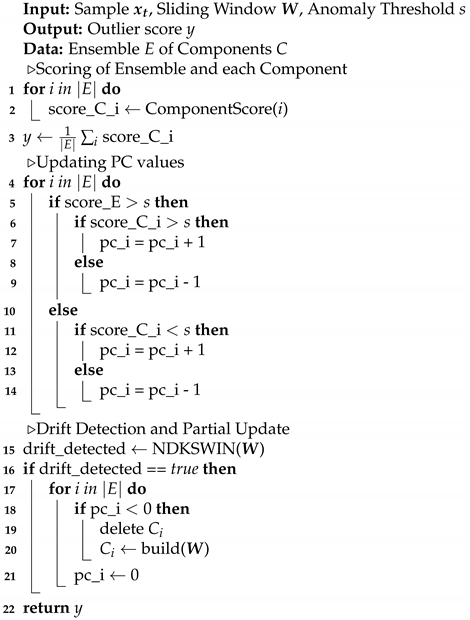
Performance Counter-Based Scoring monitors the performance of each component C (herein an iTree) in the ensemble E (herein the iForest) by assigning it with a performance counter (PC). In general, the approach favors or penalizes individual ensemble components at runtime by referring to their contributions to the ensemble’s overall scoring result. Thus, the PC-value is changed for each data instance, i.e., increased or decreased depending on the component’s scoring quality in the ensemble’s anomaly score. The PC-values increase or decrease by 1 for well and poorly performing components, depending on whether each individual score is above or under the anomaly threshold s (herein 0.5 for iForest-based learners, as discussed in [6]). For example, the ensemble scores a sample with , which indicates an anomalous sample. Each individual component’s score contribution is verified such that if the score of the i-th component is greater than s, , the PC-value of , increases. In turn, if , is penalized by decreasing . However, one might even increase or decrease the PC-values in an even more granular fashion, e.g., , depending on the confidence level of the ensemble score and each individual component’s score contribution. For instance, if , the confidence level of the ensemble is high, so the sample is anomalous. Thus, if any , component might be penalized to a larger extent by decreasing with a higher value. For the sake of simplicity in this article, we apply the more simple binary approach in which each individual PC is increased/decreased by 1 if its score value is greater/less than the ensemble’s score value. The counting goes until a drift is detected. Once this happens, the weaker performing components, as indicated by their negative PC values, are replaced with new ones built on data instances present in the current window W. The PC values of all trees are set to zero after the partial update is finished; hence, even resetting the values for previously well performing trees clears the old bias (effect of previous scoring). Referring to Figure 1, Algorithm 1 shows the working principle, including the core of the Performance Counter-Based Scoring. Additionally, we neglected the initialization phase in which, once the sliding window is filled, the components are initially built and the PC values are set to zero.
| Algorithm 1: The working principle of PCB-iForest. |
 |
4.3. Base Learner
The PCB-iForest framework is designed to allow exchanges of the base learner. Although being initially intended for iForest-based approaches, the conceptualization can easily be generalized for any ensemble method with its components, such as trees, histograms and chains. With the partial updating, unlike iForestASD and the IFA-approaches, higher throughput is possible since the complete model does not need to be updated. Rather, only a certain number of penalized trees are updated, allowing it to not completely and abruptly forget previously learned information by flushing the whole model, similarly to catastrophic interference known from the field of neural networks. Thus, with respect to non-iForest-based approaches, we see the potential of our framework to replace, e.g., the alternating windows of HS-Trees or LodaTwo Hist. in which new ensembles are built and continuously replace those currently used-even if there is no necessity. Our approach would be more resource-preserving while keeping a set of ensemble components as long as there is no need to replace them, e.g., due to a concept drift. However, in this article we focus on iForest-based approaches for the reasons stated in the beginning of this section. In particular, we want to present two application scenarios underlining the fulfillment of crucial requirements from Section 3.
4.3.1. Algorithm Agility
SD is afflicted with a theoretically infinite flow of data. Thus, in some cases, it might be necessary to exchange the base learner as time passes. A possible application scenario would be if the currently used base learner has been compromised. This means it is vulnerable to, e.g., poisoning of the algorithm, and an adversary might bypass the detection of its malicious activity. Another non-malicious use case would be a major change of data due to the long term running time that is beyond a concept drift which requires a different type of base learner. Some iForest improvements might then need tailoring for specific application scenarios. In this article, apart from classic iForest, we prove the algorithm’s agility by incorporating EIF. It addresses the drawbacks of iForest’s branching using random horizontal and vertical cuts by substituting them with non-axis-parallel hyperplanes with random slopes. Thus, to the best of our knowledge, PCB-iForest is the first work that applies the improved version of iForest on SD. Since the PCB-iForest framework only "wraps around" EIF, no other specific adaptions are necessary except for adding the Performance Counter-Based Scoring. We denote this variant as PCB-iForestEIF. However, it should be remarked that feature interpretability is irretrievably lost with the improvement of branching in EIF. Therefore, in addition, we are taking on the topic of feature importance measurement for OD on SD by a second variant explained in the next section.
4.3.2. Feature Scoring
Apart from popular dimensionality reduction algorithms such as PCA, feature selection for OD aims to only select relevant features for the classification task by discarding irrelevant and redundant features, which reduce dimensionality. This leads to more computationally efficient OD, all the while preserving feature interpretability. Especially in a consecutively applied root cause analysis, feature interpretability plays a crucial role for future forensics use cases. While some feature selection approaches only provide a subset of relevant features, others are able to score and rank features according to their contribution to a sample’s anomalousness. Therefore, one is able to select the best performing features as indicated by their score values. In particular, since iForest is inferior to projection-based methods on high-dimensional noisy datasets [18], feature selection would significantly aid in reducing dimensions, and thus, amplify iForest’s classification performance in lower dimensions. This coincides very well with the suggestion from Togbe et al. in [7], mentioning that feature selection could mitigate the effect of choosing the most important dimensions for drift detection.
Much work has been done in the field of feature selection but, to the best of our knowledge, existing approaches either focus on feature selection for SD (but not with the focus on imbalanced data classification), e.g., [45,46,47], or focus on feature selection for OD, e.g., [25,48,49], (but mainly in a supervised and offline fashion). Thus, we see it as crucial to contribute with feature scoring solutions to SD that focus on OD which might be exploited for feature selection. Pevný, in [17], proposed a one-tailed, two-sample test for Loda to achieve feature scoring without increasing its overall complexity. This approach seems most related to the intention of scoring relevant features (for the task of OD) in a streaming fashion, which one might use to rank and select the top-performing features.
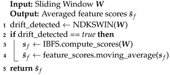
In order to achieve feature scoring, we take advantage of the unsupervised isolation-based feature selection (IBFS) method recently proposed in [25] tailored for OD. The method exploits the training phase of the classical iForest, in particular, the random selection of feature values, and computes score values for each feature by calculating imbalance scores using an entropy measure. Although this method is designed for offline iForest, it can easily be adapted to our PCB-iForest in a streaming fashion, denoted as PCB-iForestIBFS. Since it is designed for the training phase, we only obtain feature scores after each partial update (training). In order to receive representative feature scores as time passes, we will continuously update the score values with each partial update as shown in Algorithm 2. Once a partial update is triggered, we let IBFS compute feature scores for the i-th feature based on the data instances in W resulting in a one-dimensional array of d feature scores. With each partial update we continuously update the feature scores by incremental averaging. For the sake of simplicity, we apply the incremental average with a continuous counter value k for each partial update, in order to obtain the averaged array of feature scores . It must be noted that other methods exist—e.g., those discussed in [5]—that might be superior when concept drifts occur within the feature scores. While only preserving d values for the current average scores and one value for the continuous counter k and performing d updates of the scores, both the space and time complexity for each feature score averaging yields when applying the well-known Welford’s algorithm [50]. This does not significantly increase the overall complexity of PCB-iForestIBFS since d is fixed. A summary of the feature scoring functionality is shown in Algorithm 2. As time passes and feature scores are continuously computed, one might rank the feature scores and identify the top-performing ones. Thus, it might be necessary to change the feature set or reduce the number of features from the original set. PCB-iForestIBFS is able to change the feature set during runtime. Once a partial update is triggered, instead of discarding only poorly performing components, the whole model can be discarded and the new ensemble can be built using the newly proposed feature set.
| Algorithm 2: Feature scoring in PCB-iForest utilizing IBFS. |
 |
5. Experimental Evaluation
This section gives a glance at the experimental setup used for evaluation. First, the methodology is explained, followed by information on the dataset collection used and descriptions of the metrics as evaluation criteria.
5.1. Methodology and Settings
Drift detection plays a crucial role when in it comes to detecting changes that require partial updating. Thus, we (i) performed measurements to check whether NDKSWIN works within our model using dedicated datasets for drift detection. Since the most related work historically used the same set or subset of four specific datasets, we aggregated their results from the original work and (ii) performed measurements on those datasets utilizing both, PCB-iForestEIF (referring to Section 4.3.1) and PCB-iForestIBFS (referring to Section 4.3.2). A major drawback of the aforementioned is the insignificant number of multi-disciplinary datasets with an outdated, small number of dimensions in terms of today’s real-world applications. Furthermore, most of the related work from Section 2 ignores the existence of some competitors, since they included rather insignificant algorithms in their evaluations (cf. [31]). Therefore, (iii) a selection of state-of-the-art, off-the-shelf ensemble OD algorithms is compared with PCB-iForestEIF and PCB-iForestIBFS using a large collection of multi-disciplinary datasets with various dimensions. PCB-iForestIBFS performed online feature (importance) scoring. The scored features were then used in a second run on a selection of algorithms to evaluate the effects when utilizing a feature subset. Lastly, since the main application domain is network security, we (iv) evaluated our PCB-iForest variants and a selection of performant algorithms on an up-to-date dataset for network intrusion detection. It should be remarked that LSHiForestStream was not included in any of our evaluations, since it is designed for multi-dimensional multi-stream data; thus, a fair comparison is not possible within the focus of this article.
Experiments were conducted on a virtualized Ubuntu 20.04.1 LTS equipped with 12 × Intel(R) Xeon(R) CPU E5-2430 at 2.20 GHz and 32 GB memory running on a Proxmox server environment. Overall, nine off-the-shelf ensemble algorithms, including five iForest-based competitors, took part in the experiments. For equal conditions, all algorithms are coded in Python 3.7. Unless otherwise stated, the default hyperparameters of the algorithms were used and outlier thresholds fixed for all measurements. In particular, the latter seemed legitimate since one important requirement is to not burden human domain experts with complex hyperparameter settings, especially to simulate the appliance in real-world applications. For PCB-iForest we used the default parameters for NDKSWIN, as discussed in Section 6.1, and in terms of iForest, we stuck to the default parameter of an ensemble size with 100 trees and an outlier threshold of 0.5. For EIF, the fully extended version was used by setting the extension level to 1. Thus, PCB-iForest is hyperparameter-sparse and mainly affected by hyperparameter window size. However, except for Section 6.2, the window size was set to 200 for all window-using or window-based algorithms. All results (except in Section 6.1 and Section 6.4) were averaged across 10 independent runs, since most of the methods are non-deterministic, e.g., negatively affected by random projection. The UNSW-NB15 measurements in Section 6.4 were averaged across three independent runs due to the large number of instances accompanied with an enormous evaluation-runtime for some inefficient classifiers.
5.2. Data Sources
To achieve high quality in our evaluation, we utilized four different dataset sources. In order to measure the performance of NDKSWIN, we utilized the recently proposed ensemble of synthetic datasets for concept drift detection purposes from the Harvard Dataverse [51]. It contains 10 abrupt and 10 gradual datasets, each consisting of approximately 40,000 instances and the same three locations where abrupt and gradual drifts were injected. In particular, rt_2563789698568873_abrupto and rt_2563789698568873_gradual were used in our evaluation.
Since some of the iForest-related work performed measurements on four of the datasets used in [26], we stuck to this approach and performed measurements using PCB-iForest on HTTP, SMTP (from security-related KDD Cup 99 (http://kdd.ics.uci.edu/databases/kddcup99/kddcup99.html, accessed on 12 May 2021)), ForestCover and Shuttle (from UCI Machine Learning Repository [52]) datasets. We truncated the datasets varying in number of samples while keeping their outlier percentages as in the original sets (HTTP—0.39%, SMTP—0.03%, ForestCover—0.96%, Shuttle—7.15%) in order to reduce processing runtime. In the following, the four datasets are denoted as HSFS.
In recent years, the majority of state-of-the-art IDS datasets, including KDD Cup 99 and its improved successor NSL-KDD (https://www.unb.ca/cic/datasets/nsl.html, accessed on 12 May 2021), have been criticized by many researchers since their data are out of date or do not represent the threat landscape of today [53,54]. Therefore, we have chosen two improvements compared to the aforementioned evaluation datasets. First, we have selected fifteen real-world candidate datasets from the Outlier Detection DataSets (ODDS) Library (http://odds.cs.stonybrook.edu/about-odds/, accessed on 12 May 2021) [55] tailored for the purpose of OD. Those will serve to benchmark PCB-iForest in terms of a variety of different amounts of features, contrasting outlier percentages and the application across multi-disciplinary domains. In particular, we included the ensemble of datasets from ODDS shown in Table 2 with their characteristics. To reduce the processing runtime of each OD algorithm, mnist, musk, optdigits, pendigits, satellite, satimage-2 and shuttle were truncated while mostly maintaining their original outlier percentages.
Table 2.
Characteristics of the partially truncated datasets from ODDS [55].
Even though CSE-CIC-IDS2018 (https://registry.opendata.aws/cse-cic-ids2018/, accessed on 12 May 2021) overcomes most of the aforementioned criticism and is said to be well designed and maintained [54], in terms of a network security related dataset, we have selected its competitor UNSW-NB15 [56] for the following reasons. It is also well structured, and labeled, and more complex than many other security-related datasets, making it a useful benchmark for evaluation [54]. However, apart from the proneness to the issue of high-class imbalance for CSE-CIC-IDS2018 mentioned in a recent publication [57], the main reason for choosing UNSW-NB15 is that the aggregated datasets contain the IP address (source and destination), and the respective port features, which we deem essential for a consecutively applied root cause analysis. Especially, similarity-based alert analysis approaches such as [58] cannot be utilized when those features are missing, since they mainly operate on this information.
UNSW-NB15 incorporates nine types of attacks, namely, fuzzers, analysis attacks, backdoor attacks, DoSs, exploits, generic attacks, reconnaissance, shellcode and worms created by the IXIA PerfectStorm tool. In terms of feature generation, Argus and Bro-IDS tools, among others, were utilized to generate 49 features which can be divided into five feature sets: flow, basic, content, time and additional. Since the four CSV files available only contain the raw features, further data preparation steps had to be performed, including handling inconsistent values, dropping irrelevant features and dealing with categorical attributes. Sanitizing had to be performed for source and destination port features containing some values that did not conform with others. Hexadecimal values were converted to integers, and for ICMP-protocol-based features, some values containing the character “-” were set to zero. Empty string values were replaced by 0 and typecast according to their column types defined in [56]. We dropped the timestamp feature, since it has no added value for OD, albeit important for a consecutive root cause analysis. However, in real-world scenarios the timestamp will be added after the detection of outliers, since it is not contained in the incoming data.
Except for srcip, sport, dstip, dsport, proto, state and service (we do not count the actual binary prediction label and the attack category), the datasets contained only numerical and binary data, which could be processed by the applied OD algorithms. Various methods can be applied to handle IP-addresses, such as converting them into their binary or integer representations (one-to-one), splitting them into four numbers (one-to-four) or applying the widely-used one-hot encoding for categorical features (one-to-many). However, the latter is not feasible in the real-world online setting since (i) all possible IP-addresses that might occur must be known in advance and (ii) one-hot encoding leads to a significantly higher number of features. We chose to convert the IP-addresses into integers, since it is an acceptable option for network intrusion detection [59] and does not increase the number of dimensions. The port feature can easily be converted into an integer, and for proto, state and service, one-hot encoding was used such that the number of features did not grow too large and could be utilized on SD. Other than, e.g., proto, only TCP and UDP have the largest proportions; categories have been limited to only the most important ones in terms of frequency by merging the least occurring values into one category (beneath 1% occurrence). A domain expert could also predefine those categories based on domain knowledge. By this method, the generated feature space of the whole dataset could be reduced from 207 to finally 57 features. The four sanitized CSV files with its characteristics are summarized in Table 3.
Table 3.
Characteristics of the four preprocessed CSV files from the UNSW-NB15 dataset [56].
5.3. Evaluation Criteria
The confusion matrix, consisting of the parameters true negatives (), false negatives (), false positives () and true positives (), is the most intuitive and widely-used performance measure for binary classification of machine learning algorithms. Further parameters can be derived, such as accuracy, precision, recall or specificity. The most widely used as the standard metric for the score-wise evaluation of outlier detectors is of the receiver operating characteristic () curve. is created by plotting the true positive rate (), meaning the recall against the false positive rate (), which corresponds to 1-specificity. is computed by and by . The metric is used for the sake of comparing related work results in Table 4. It is computed as as proposed in [60].
Table 4.
Classification performances of different iForest-based competitors aggregated from their respective original works with PCB-iForestEIF and PCB-iForestIBFS (* best setting with ; best performing values in bold).
The harmonic mean of precision and recall, denoted as score, is used for representation of the classification performance for all other measurements. It can be computed as . Compared to , we deem the score more appropriate for OD since, e.g., the used in the metric depends on the number of whose proportion in OD is typically quite large. Thus, the tends to be near 1 when classifying imbalanced data, and thus, is not the best measure for examining OD algorithms. A good indicates low and and is therefore a better choice to reliably identify malicious activity in the network security domain without being negatively impacted by false alarms.
Furthermore, we measured the average runtime per OD algorithm, denoted as , as a representative metric for the computational performance. Thus, we accumulated the elapsed time for individual steps necessary to perform, e.g., partial fitting or prediction, to derive the average runtime after multiple iterations for processing a particular dataset. Providing a tradeoff between the classification and computational performance, the last metric is the ratio of .
6. Discussion of Results
In this section we discuss some of the key results obtained by the comprehensive evaluation. It is structured in the following parts. We discuss the capability of PCB-iForest’s drift detection by examining NDKSWIN. Then, PCB-iForestEIF and PCB-iForestIBFS are extensively evaluated against related work in the following sections. This includes three different types of data sources and includes the evaluation of the feature importance scoring functionality by PCB-iForestIBFS.
6.1. NDKSWIN Drift Detection
NDKSWIN drift detection is mainly affected by the hyperparameters sliding window size w, the number of samples to be tested as a percentage value of the window size, sub-window size for the latest samples r, the number of dimensions to be evaluated and the -value of the KS-test. For the sake of low hyperparameter complexity, we will rely on the default values , , and used in [7]. Since the sliding window size is a crucial parameter, not only for NDKSWIN but also for PCB-iForest, this section examines possible effects of slightly varying hyperparameters of NDKSWIN and discusses potential impacts on PCB-iForest. Since marginal changes in did not remarkably influence the results, we varied parameters with the sets , , and .
Across all measurements, NDKSWIN was mostly able to detect the gradual and abrupt drifts but was afflicted to a high number of false detections as exemplary shown in Figure 2 with two different settings. The duration of a gradual drift lasted for 1000 samples, which is indicated by rectangles in gray. The sliding window size is indicated by rectangles in red which apply to gradual and abrupt drift detection. The actual detected drift location can only be pinpointed within the range of a window. Thus, detected gradual drifts were counted if either the gray or the red rectangle was intersecting, and the abrupt drift had to be detected near the red rectangle. In general, from the 24 measurements with the varying settings, NDKSWIN was able to detect 61 out of 72 gradual and 40 out of 72 abrupt drifts.
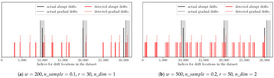
Figure 2.
Exemplary visualization of NDKSWIN gradual and abrupt drift detection with two different hyperparameter settings (rectangles in gray—duration of gradual drift; rectangles in red—sliding window size).
Generally, by increasing NDKSWIN’s hyperparameters, multiple tests performed for many dimensions led to increasing probability of falsely detected drifts for one dimension, although none was present. This phenomenon might be reasoned due to the widely known problem in statistics called multiple comparison or multiple testing. Independent of the window size, this problem is more distinct for higher values , r and , as shown in an exemplary way in Figure 2a,b. To strengthen our assumption, we have varied , r and each at a time while observing the change in false detections. Its number was higher every time we increased each value. In particular, increasing from 0.1 to 0.2 while keeping the other hyperparameters stable resulted in a doubling of false detections. In turn, increasing r (30 to 50) and (1 to 2) led to approximate increases of 40% in false detections. The problem can be alleviated by choosing small hyperparameter values. Thus, the default parameters proposed in [7] , , and achieved decent results and mostly mitigated the multiple comparisons problem for its small values and were therefore used in our further measurements.
Since the performed measurements are only non-deterministic snapshots without averaging the results over multiple runs, more intensive measurements for drift detection are necessary in future work. We deliberately chose to not average the results, since this would blur the results in terms of actual drift detection and would not show the effects in real-world applications. Future measurements will include the comparison to other data-centric drift detection methods and take into account higher dimensional datasets. Furthermore, we want to focus on improving the NDKSWIN method by tackling the proneness to the multiple comparisons problem. Although drift detection plays a crucial role in our model, it is not the main focus of our article. We conclude from the measurements that NDKSWIN is able to reliably detect actual drifts and regularly updates our model when triggered by falsely detected drifts. However, it should be remarked that the used datasets lack information regarding the drift characteristics, meaning how distinct drifts are to be detected. For the rest of our evaluation, we set the default parameters (except for the window size) to achieve a good tradeoff between updating our model in regular times and not demanding extensive resources by continuously updating it with every sample.
6.2. Competitor-Based HSFS
PCB-iForestEIF and PCB-iForestIBFS were evaluated on the HSFS datasets used by some of the iForest-based competitors: iForestASD, IFA(S/P)ADWIN and IFANDKSWIN and GR-Trees. Table 4 shows the results; the best-performing values from the competitors’ original work have been included together with the measurement results for the two PCB-iForest versions using different window sizes w. Although Togbe et al. in [7] used all four datasets to compare HS-Trees and iForestASD, they only performed measurements on Shuttle and SMTP utilizing IFA(S/P)ADWIN and IFANDKSWIN. What is more, contrary to iForestASD and GR-Trees, the authors chose the instead of metric. Since we included Shuttle in our ODDS measurements in the next section and also relied on the , only the results from iForestASD and GR-Trees are presented. It must be noted that the authors of GR-Trees constrained the abnormal proportion of each dataset to 10% in their evaluation. This step can be seen as critical since the datasets normally have outlier percentages between 0.03% and 7.15% so that classification results can be blurred by this step. Despite that, GR-Trees performed inferiorly to iForestASD and both PCB-iForest versions, as shown in Table 4. For this reason, GR-Trees was excluded from the rest of our measurements. As expected, with its showing an improvement over the outlier scoring of iForest, PCB-iForestEIF yielded the best results in most cases except for HTTP. PCB-iForestIBFS achieved very good results on HTTP across all window sizes. Though it was outperformed by both PCB-iForest variants on three datasets, iForestASD achieved decent results. However, it is firstly remarked that the predefined threshold parameter used to trigger concept drifts, and thus update the iForestASD model, depends on a priori knowledge, thereby limiting its applicability in real-world scenarios. Secondly, the measurements did not take into account computational performance, since we assumed that iForestASD performs much worse than our PCB-iForest, which is able to partially update its model. We discuss the results of our tradeoff measurements between classification and computational performance in the next section.
6.3. Multi-Disciplinary ODDS
Since in real-world applications, hyperparamater optimization is difficult, especially on SD afflicted with concept drifts, we compared the results of several off-the-shelf, state-of-the-art OD algorithms with our proposed PCB-iForest versions using the default parameters proposed in the respective original work and across multi-disciplinary datasets with varying characteristics.
6.3.1. Full Dimensions
First, we ran each classifier on full dimensions. Later, the effects of PCB-iForestIBFS’s feature importance scoring using a subset of the best-performing features applied on different algorithms were evaluated. The results of the metric are shown in Table 5. In approximately half of the datasets, PCB-iForestEIF outperformed the other online OD algorithms by achieving the best classification result, and hence achieved the first rank averaged over all datasets. Other than datasets with IDs 7, 10 and 11, PCB-iForestEIF performed at least comparably with the other datasets, and PCB-iForestIBFS only marginally performed worse, with an overall rank 3, being only slightly outperformed by iMForest. All iForest-based competitors achieved similar averaged outlier scores, taking the rankings 6–9.
Table 5.
results for different online OD algorithms on datasets with ID i (best performing values in bold; “-”, measurement aborted after 42 h runtime; denotes the average outlier score over all datasets; , from best (1) to worst (11) performance).
However, considering the slightly better average runtime, PCB-iForestIBFS outperformed PCB-iForestEIF in terms of in almost all measurements, as depicted on two exemplary datasets mnist and optdigits in Figure 3, thereby presenting itself as an OD algorithm with a good tradeoff between classification performance and computational costs. Except for those two datasets, LodaTwo Hist. achieved the best results across all online OD algorithms, as shown in Table 6, summarizing the results. Except for the efficiently performing LodaTwo Hist. on rank 1, our proposed PCB-iForestIBFS and PCB-iForestEIF showed consistently remarkable results with rank 2 and 3, even superior to the well performing iMForest with respect to its results. Table 6 also shows the inefficient processing of the iForest-based competitors; in particular, the IFA variants took ranks 7–9 evenly and iForestASD the last rank.
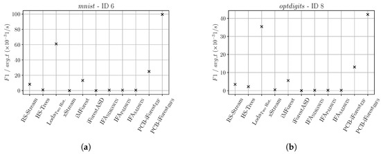
Table 6.
results for different online OD algorithms on datasets with ID i (best performing values in bold; “-”, measurement aborted after 42 h runtime; denotes the average outlier score over all datasets; , from best (1) to worst (11) performance; values are scaled by a factor of in units of 1/s).
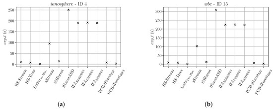
In most of the measurements, iForestASD yielded the longest value followed by IFANDKSWIN and IFA(S/P)ADWIN and xStream. The results for two exemplary datasets ionosphere and wbc are shown in Figure 4. It should be remarked that for datasets letter, satellite and shuttle the exceeded 4 hours per dataset iteration due to the extensive runtime of those four classifiers. Therefore, we excluded them from the remainder of our evaluation.
6.3.2. Feature Subsets
Due to the extensive runtime of some classifiers, we continued our evaluation using RS-Hash, HS-Trees, iMForest, LodaTwo Hist. and our two PCB-iForest variants to evaluate the online-capable feature importance scoring functionality of PCB-iForestIBFS. Thus, we used the scored feature values obtained by PCB-iForestIBFS, ranked them and supplied subsets of 25%, 50% and 75% to each online OD algorithm. Ideally, if feature scoring operates correctly, the subset of features on the one hand yields a more precise classification result, while on the other hand, the computational effort can be limited by minimizing the cardinality of the selected feature set. Thus, the metric should tend to achieve better results using a subset compared to the full dimension measurements with all features in average across all algorithms. This can also be seen from the results in Table 7. The full feature set is only top performing for 5 datasets while applied feature subsets yield the best result for 10 datasets. Since, to the best of our knowledge, (as of now) no other online unsupervised feature selection method for OD exists, we could not cross-check our results. In addition no ground truth information is available for ODDS revealing details on which features mainly cause outliers. Thus, with respect to the 5 badly-performing datasets (ID 10–13 and 15), outliers tend to occur in a wide range of dimensions leading to a higher degradation using a subset than benefiting from the reduction, thus, resulting in a worse . This effect is strengthened by Table 7 showing that higher numbers of features in a subset for the badly-performing datasets generally resulted higher . Likewise, without ground truth information, it cannot be shown that for the 67% well-performing datasets, subsets from 25–75% of the features caused the majority of outliers and thus resulted in good values. Nevertheless, the focus of the feature selection results should be set on the high-dimensional datasets, such as arrhythmia, mnist and musk with IDs 1, 6 and 7, since as stated and discussed in [18] most of the classifiers can efficiently handle lower dimensions. For those datasets all feature subsets achieved better results than full dimension.
Table 7.
results averaged for each online OD using different feature sets for datasets with ID i (full_dimension refers to using all features; *_25,50,75 refers to using the top scoring 25%, 50% and 75% features obtained by PCB-iForestIBFS; top performing values bold; values are scaled by a factor of in units of 1/s).
A better picture of the good performance shown in an exemplarily way for high-dimensional arrhythmia and musk, can be obtained by examining the feature scores , as shown in Figure 5. Having a high number of dimensions, feature selection can significantly aid to reduce them, which in turn increases a classifier’s classification performance while reducing its computational cost only processing relevant features for the purpose of OD. With regard to the score results for arrhythmia and musk, as shown in Figure 6, 50% of the 274 features from arrhythmia are already sufficient for achieving better results than utilizing the full feature set. For musk, the same applies at the 25% mark of the 166 features.
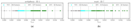
Figure 5.
Exemplary plots for feature scores on the high-dimensional arrhythmia (a) and musk (b), including 25%, 50% and 75% subsets, shown in different colors.
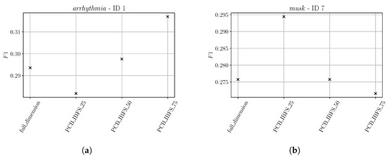
Figure 6.
results for the high-dimensional datasets arrhythmia (a) and musk (b) utilizing different feature sets (full_dimension refers to using all features. *_25,50,75 refers to using the top scoring 25%, 50% and 75% features obtained by PCB-iForestIBFS).
In order to show the influence of applying a feature set to each classifier, we refer to Table 8 showing the percentage increase/decrease of and when applying a feature subset compared to full dimension on the arrhythmia and musk dataset. Except for PCB-iForestIBFS on both datasets and HS-Trees on musk, the could be reduced for all classifiers. Generally, the average runtime could be reduced by approximately 6% on arrhythmia and 9% on musk. Contrary to PCB-iForestIBFS, as expected, PCB-iForestEIF significantly benefits by the dimensionality reduction for both datasets. In terms of , again we see a performance degradation for PCB-iForestIBFS but a significant increase for PCB-iForestEIF on both datasets, especially musk. Generally, the performance could be increased by approximately 11% on arrhythmia and 30% on musk. Excluding the high value achieved by PCB-iForestEIF on musk, the percentage increase is still notable with an increase of 5%. The poor performance of PCB-iForestIBFS utilizing a feature subset only takes place for those two datasets and wbc. On all other datasets, PCB-iForestIBFS could increase the while additionally reducing the with at least one of the subsets. Although being a projection-based method that is designed to operate on high-dimensional datasets, LodaTwo Hist. achieves performance boosts on both high-dimensional datasets, arrhythmia and musk, for and . In summary, it can be said that each individual method reacts differently to feature subsets and although the performance partially degrades for some of them, the overall benefit by a combination of classifiers is clearly evident.
Table 8.
Individual classifier performance in terms of the percentage increases/decreases of and when applying a feature subset compared to full dimensions on the arrhythmia and musk datasets.
6.4. Security-Related UNSW-NB15
The results of the time intensive processing-running approximately 38 h-of the four UNSW-NB15 CSV files for only 3 iterations utilizing 6 online OD methods are presented in Table 9. Again, LodaTwo Hist. achieves the best results across all measurements for the resulting in a notable 1.0 ms to process one data instance. This is faster by a factor of approximately 15 compared to the slowest algorithms, iMForest and RS-Stream, achieving approximately 15 ms. For HS-Trees it takes approximately 11.6 ms and for PCB-iForestEIF 5.6 ms to process one sample. Remarkably, PCB-iForestIBFS operates most competitively to LodaTwo Hist. with 1.6 ms. Albeit processing samples very efficiently, with respect to the metric, LodaTwo Hist. could only outperform our proposed PCB-iForestIBFS for CSV files #1 and #3.
Table 9.
and results for different online OD algorithms on the four preprocessed CSV files from the UNSW-NB15 dataset (best performing values in bold).
In terms of , our proposed PCB-iForest variants outperform the other classifiers on all four CSV files except for #1 where all algorithms performed poorly. The reason behind this poor performance on #1 might be the slightly different distribution of attack categories and the high imbalance of normal and abnormal data. The generic attack category has the highest proportion of all other classes, on all files. However, on file #2–#4 the proportion of the generic class is higher with approximately 4% on #2, 17% on #3 and 14% on #3 compared to only approximately 1% on #1. Furthermore, the higher proportion of normal data with approximately 97% on #1 compared to 92% on #2, 78% on #3, 80% on #4 leads, in general, to poorer values due to the extreme imbalance of positive and negative classes [61].
7. Conclusions and Future Work
Over the past few years, the continuous increase in high-volume, high-speed and high-dimensional unlabeled streaming data has pushed the development of anomaly detection schemes across multiple domains. Those require efficient unsupervised and online processing capable of dealing with challenges such as concept drift. The most popular state-of-the-art outlier detection methods for streaming data were discussed in this paper, with a focus on algorithms based on the widely known isolation forest (iForest), and they were compared against thoroughly engineered requirements pointing out the lack of a flexible, robust and future-oriented solution.
Thus, this article introduces and discusses a novel framework called PCB-iForest that “wraps around”, generically, any ensemble-based online OD method. However, due to its popularity, the main focus lies on the incorporation of iForest-based methods for which we present two variants. PCB-iForestEIF is (to the best of our knowledge) the first application of the iForest improvement called extended isolation forest on streaming data. PCB-iForestIBFS applies a recently proposed feature importance scoring functionality designed for static data, which is adapted to function in a streaming fashion. We provide details of PCB-iForest’s core functionality based on performance counters assigned to each ensemble component in order to favor or penalize well or poorly performing components. The latter will be replaced if concept drifts are detected by newly built ones based on samples within a sliding window. Since drift detection is crucial, in order to regularly update our model if required, we rely on a recently proposed method denoted as NDKSWIN, but are open to any multi-dimensional data-centric method.
Our extensive evaluation firstly evaluated the drift detection functionality, which showed that NDKSWIN is able to detect concept drifts, and even if afflicted by some additional detections, regularly updates PCB-iForest. Comprehensively comparing both PCB-iForest methods with state-of-the-art competitors pointed out the superiority of our method in most cases. In terms of area under the receiver operating characteristic () curve, we achieved the best results on four datasets used by online iForest-based competitors. On the multi-disciplinary ODDS, PCB-iForest clearly outperformed nine competitors in approximately 50% of the datasets and achieved comparable results in 80% with respect to the metric and its tradeoff with the average runtime. Utilizing the four most efficient competitors and our PCB-iForest variants on four security-related UNSW-NB15 datasets again proved the superiority of our approach. It achieved the highest (we do not include the poor performance of all classifiers on one dataset) while still being comparable in speed to the extremely fast Loda algorithm.
PCB-iForest’s current implementation faces two limitations which will be addressed as part of future work by taking advantage of the framework’s flexible design to incorporate other ensemble-based OD algorithms and replacing the drift detection method. Thus, firstly, we will focus on the integration of LodaTwo Hist. into PCB-iForest, given (i) its rapid processing and (ii) the fact that its classification results could be further improved by replacing the pair of alternating windows with our approach. Therefore, the set of histograms will only partially be replaced if concept drift is detected and will not completely be discarded after each window.
Secondly, drift detection is a crucial component of our approach, since it must reliably detects concept drifts and should not be prone to a high number of false detections, because this would degrade both the classification and computational performance. Therefore, our future work will (i) focus on the improvement of NDKSWIN, since it is possibly prone to the multiple comparisons problem, and (ii) evaluate the use of other multi-dimensional data-centric algorithms within PCB-iForest.
More research will also be part of PCB-iForestIBFS’s feature scoring functionality, since even if it is able to score and rank the best-performing features during runtime, determining the “optimum” number of features that should be used as a feature subset is still an open issue. Although the subsets with 25–75% of the whole feature set could achieve promising results, this is highly dependent on the data source and algorithm type. Thus, a method will be developed that determines the best feature subset based on the analysis of the feature scores.
Author Contributions
Conceptualization, M.H.; methodology, M.H. and K.A.A.; Software, M.H., K.A.A., A.U.; validation, M.H., D.F. and R.H.; writing—original draft, M.H.; visualization, M.H., K.A.A. and A.U.; writing—review and editing, M.H., D.F., M.S. and R.H.; supervision, D.F., M.S. and R.H.; funding acquisition, D.F. and M.S.; project administration, M.S. All authors have read and agreed to the published version of the manuscript.
Funding
This research work is partially supported by the research project 13FH645IB6 of the German Federal Ministry of Education and Research; and by the Ministry of Education, Youth and Sports of the Czech Republic under grant number LO1506.
Conflicts of Interest
The authors declare no conflict of interest.
References
- Liu, H.; Lang, B. Machine learning and deep learning methods for intrusion detection systems: A survey. Appl. Sci. 2019, 9, 4396. [Google Scholar] [CrossRef] [Green Version]
- Ramaki, A.A.; Rasoolzadegan, A.; Bafghi, A.G. A systematic mapping study on intrusion alert analysis in intrusion detection systems. ACM Comput. Surv. 2018, 51, 1–41. [Google Scholar] [CrossRef]
- Nespoli, P.; Papamartzivanos, D.; Gomez Marmol, F.; Kambourakis, G. Optimal countermeasures selection against cyber attacks: A comprehensive survey on reaction frameworks. IEEE Commun. Surv. Tutor. 2018, 20, 1361–1396. [Google Scholar] [CrossRef]
- Ahmad, S.; Lavin, A.; Purdy, S.; Agha, Z. Unsupervised real-time anomaly detection for streaming data. Neurocomputing 2017, 262, 134–147. [Google Scholar] [CrossRef]
- Reunanen, N.; Räty, T.; Jokinen, J.J.; Hoyt, T. Unsupervised online detection and prediction of outliers in streams of sensor data. Int. J. Data Sci. Anal. 2020, 9, 285–314. [Google Scholar] [CrossRef] [Green Version]
- Liu, F.T.; Ting, K.M.; Zhou, Z.-H. Isolation Forest. In Proceedings of the 2008 Eighth IEEE International Conference on Data Mining, Pisa, Italy, 15–19 December 2008; pp. 413–422. [Google Scholar] [CrossRef]
- Togbe, M.U.; Chabchoub, Y.; Boly, A.; Barry, M.; Chiky, R.; Bahri, M. Anomalies detection using isolation in concept-drifting data streams. Computers 2021, 10, 13. [Google Scholar] [CrossRef]
- Pang, G.; Cao, L.; Chen, L.; Liu, H. Unsupervised feature selection for outlier detection by modelling hierarchical value-feature couplings. In Proceedings of the 2016 IEEE 16th International Conference on Data Mining (ICDM), Barcelona, Spain, 12–15 December 2016; pp. 410–419. [Google Scholar] [CrossRef] [Green Version]
- Muallem, A.; Shetty, S.; Pan, J.W.; Zhao, J.; Biswal, B. Hoeffding tree algorithms for anomaly detection in streaming datasets: A survey. J. Inf. Secur. 2017, 8, 339–361. [Google Scholar] [CrossRef] [Green Version]
- Saffari, A.; Leistner, C.; Santner, J.; Godec, M.; Bischof, H. On-line random forests. In Proceedings of the 2009 IEEE 12th International Conference on Computer Vision Workshops, ICCV Workshops, Kyoto, Japan, 27 September–4 October 2009; pp. 1393–1400. [Google Scholar] [CrossRef]
- Liu, L.; Hu, M.; Kang, C.; Li, X. Unsupervised anomaly detection for network data streams in industrial control systems. Information 2020, 11, 105. [Google Scholar] [CrossRef] [Green Version]
- Yao, H.; Fu, X.; Yang, Y.; Postolache, O. An incremental local outlier detection method in the data stream. Appl. Sci. 2018, 8, 1248. [Google Scholar] [CrossRef] [Green Version]
- Mirsky, Y.; Doitshman, T.; Elovici, Y.; Shabtai, A. Kitsune: An ensemble of autoencoders for online network intrusion detection. In Proceedings of the Network and Distributed System Security Symposium 2018 (NDSS’18), San Diego, CA, USA, 18–21 February 2018. [Google Scholar]
- Yu, K.; Shi, W.; Santoro, N. Designing a streaming algorithm for outlier detection in data mining—An incremental approach. Sensors 2020, 20, 1261. [Google Scholar] [CrossRef] [Green Version]
- Tan, S.C.; Ting, K.M.; Liu, T.F. Fast anomaly detection for streaming data. In Proceedings of the Twenty-Second international joint conference on Artificial Intelligence-Volume Two, Barcelona, Catalonia, Spain, 16–22 July 2011; AAAI Press: Menlo Park, CA, USA, 2011; pp. 1511–1516. [Google Scholar] [CrossRef]
- Sathe, S.; Aggarwal, C.C. Subspace outlier detection in linear time with randomized hashing. In Proceedings of the 2016 IEEE 16th International Conference on Data Mining (ICDM), Barcelona, Spain, 12–15 December 2016; pp. 459–468. [Google Scholar] [CrossRef]
- Pevný, T. Loda: Lightweight on-line detector of anomalies. Mach. Learn. 2016, 102, 275–304. [Google Scholar] [CrossRef] [Green Version]
- Manzoor, E.; Lamba, H.; Akoglu, L. xStream: Outlier detection in feature-evolving data streams. In Proceedings of the Proceedings of the 24th ACM SIGKDD International Conference on Knowledge DiscoveryData Mining, London, UK, 19–23 August 2018; ACM: New York, NY, USA, 2018. [Google Scholar] [CrossRef]
- Aggarwal, C.C.; Sathe, S. Theoretical foundations and algorithms for outlier ensembles. SIGKDD Explor. 2015, 17, 24–47. [Google Scholar] [CrossRef]
- Aggarwal, C.C. High-dimensional outlier detection: The subspace method. In Outlier Analysis; Springer International Publishing: Cham, Switzerland, 2017; pp. 149–184. [Google Scholar] [CrossRef]
- Ben-Haim, Y.; Tom-Tov, E. A streaming parallel decision tree algorithm. J. Mach. Learn. Res. 2010, 11, 849–872. [Google Scholar]
- Fernández-Delgado, M.; Cernadas, E.; Barro, S.; Amorim, D. Do we need hundreds of classifiers to solve real world classification problems? J. Mach. Learn. Res. 2014, 15, 3133–3181. [Google Scholar]
- Hariri, S.; Carrasco Kind, M.; Brunner, R.J. Extended Isolation Forest. IEEE Trans. Knowl. Data Eng. 2019, 33, 1479–1489. [Google Scholar] [CrossRef] [Green Version]
- Staerman, G.; Mozharovskyi, P.; Clémençon, S.; d’Alché-Buc, F. Functional Isolation Forest. In Proceedings of the Eleventh Asian Conference on Machine Learning, Nagoya, Japan, 17–19 November 2019; pp. 332–347. [Google Scholar]
- Yang, Q.; Singh, J.; Lee, J. Isolation-based feature Selection for Unsupervised Outlier Detection. Proc. Annu. Conf. Progn. Health Manag. Soc. 2019, 11. [Google Scholar] [CrossRef]
- Ding, Z.; Fei, M. An anomaly detection approach based on isolation forest algorithm for streaming data using sliding window. IFAC Proc. 2013, 46, 12–17. [Google Scholar] [CrossRef]
- Togbe, M.U.; Barry, M.; Boly, A.; Chabchoub, Y.; Chiky, R.; Montiel, J.; Tran, V.-T. Anomaly detection for data streams based on isolation forest using scikit-multiflow. In Computational Science and Its Applications—ICCSA 2020; Springer International Publishing: Cham, Switzerland, 2020; pp. 15–30. [Google Scholar] [CrossRef]
- Bifet, A.; Gavaldà, R. Adaptive learning from evolving data streams. In Advances in Intelligent Data Analysis VIII; Springer: Berlin/Heidelberg, Germany, 2009; pp. 249–260. [Google Scholar] [CrossRef]
- Raab, C.; Heusinger, M.; Schleif, F.-M. Reactive soft prototype computing for concept drift streams. Neurocomputing 2020, 416, 340–351. [Google Scholar] [CrossRef]
- Sun, H.; He, Q.; Liao, K.; Sellis, T.; Guo, L.; Zhang, X.; Shen, J.; Chen, F. Fast anomaly detection in multiple multi-dimensional data streams. In Proceedings of the 2019 IEEE International Conference on Big Data (Big Data), Los Angeles, CA, USA, 9–12 December 2019; pp. 1218–1223. [Google Scholar] [CrossRef]
- Ma, H.; Ghojogh, B.; Samad, M.N.; Zheng, D.; Crowley, M. Isolation Mondrian forest for batch and online anomaly detection. In Proceedings of the 2020 IEEE International Conference on Systems, Man, and Cybernetics (SMC), Toronto, ON, Canada, 11–14 October 2020; pp. 3051–3058. [Google Scholar] [CrossRef]
- Zöller, M.-A.; Huber, M.F. Benchmark and survey of automated machine learning frameworks. J. Artif. Intell. Res. 2021, 70, 409–472. [Google Scholar] [CrossRef]
- Krawczyk, B.; Cano, A. Online ensemble learning with abstaining classifiers for drifting and noisy data streams. Appl. Soft Comput. 2018, 68, 677–692. [Google Scholar] [CrossRef]
- Iglesias, F.; Zseby, T. Analysis of network traffic features for anomaly detection. Mach. Learn. 2015, 101, 59–84. [Google Scholar] [CrossRef] [Green Version]
- Goodfellow, I.; McDaniel, P.; Papernot, N. Making machine learning robust against adversarial inputs. Commun. ACM 2018, 61, 56–66. [Google Scholar] [CrossRef]
- Kianpour, M.; Wen, S.-F. Timing attacks on machine learning: State of the art. In Advances in Intelligent Systems and Computing; Springer International Publishing: Cham, Switzerland, 2020; pp. 111–125. [Google Scholar] [CrossRef]
- Liao, L.; Luo, B. Entropy isolation forest based on dimension entropy for anomaly detection. InCommunications in Computer and Information Science; Springer: Singapore, 2019; pp. 365–376. [Google Scholar] [CrossRef]
- Zhang, X.; Dou, W.; He, Q.; Zhou, R.; Leckie, C.; Kotagiri, R.; Salcic, Z. LSHiForest: A generic framework for fast tree isolation based ensemble anomaly analysis. In Proceedings of the 2017 IEEE 33rd International Conference on Data Engineering (ICDE), San Diego, CA, USA, 19–22 April 2017; pp. 983–994. [Google Scholar] [CrossRef]
- Xu, D.; Wang, Y.; Meng, Y.; Zhang, Z. An improved data anomaly detection method based on isolation forest. In Proceedings of the 2017 10th International Symposium on Computational Intelligence and Design (ISCID), Hangzhou, China, 9–10 December 2017; Volume 2, pp. 287–291. [Google Scholar] [CrossRef]
- Cortes, D. Distance approximation using Isolation Forests. arXiv 2019, arXiv:1910.12362. [Google Scholar]
- Gama, J.; Medas, P.; Castillo, G.; Rodrigues, P. Learning with drift detection. In Advances in Artificial Intelligence—SBIA 2004; Springer: Berlin/Heidelberg, Germany, 2004; pp. 286–295. [Google Scholar] [CrossRef]
- Bifet, A.; Gavaldà, R. Learning from time-changing data with adaptive windowing. In Proceedings of the 2007 SIAM International Conference on Data Mining, Minneapolis, MN, USA, 26–28 April 2007; Society for Industrial and Applied Mathematics: Philadelphia, PA, USA; Volume 7, pp. 443–448. [Google Scholar] [CrossRef] [Green Version]
- Dasu, T.; Krishnan, S.; Lin, D.; Venkatasubramanian, S.; Yi, K. Change (detection) you can believe in: Finding distributional shifts in data streams. In Advances in Intelligent Data Analysis VIII; Springer: Berlin/Heidelberg, Germany, 2009; pp. 21–34. [Google Scholar] [CrossRef]
- Kuncheva, L.I. Change detection in streaming multivariate data using likelihood detectors. IEEE Trans. Knowl. Data Eng. 2013, 25, 1175–1180. [Google Scholar] [CrossRef]
- Shao, W.; He, L.; Lu, C.-T.; Wei, X.; Yu, P.S. Online Unsupervised Multi-view Feature Selection. In Proceedings of the 2016 IEEE 16th International Conference on Data Mining (ICDM), Barcelona, Spain, 12–15 December 2016; pp. 1203–1208. [Google Scholar] [CrossRef] [Green Version]
- Hammoodi, M.S.; Stahl, F.; Badii, A. Real-time feature selection technique with concept drift detection using adaptive micro-clusters for data stream mining. Knowl. Based Syst. 2018, 161, 205–239. [Google Scholar] [CrossRef] [Green Version]
- Renuka, D.; Sasikala, S. Online Feature Selection (OFS) with Accelerated Bat Algorithm (ABA) and Ensemble Incremental Deep Multiple Layer Perceptron (EIDMLP) for big data streams. J. Big Data 2019, 6, 103. [Google Scholar] [CrossRef] [Green Version]
- Zhang, H.; Nian, K.; Coleman, T.F.; Li, Y. Spectral ranking and unsupervised feature selection for point, collective, and contextual anomaly detection. Int. J. Data Sci. Anal. 2020, 9, 57–75. [Google Scholar] [CrossRef] [Green Version]
- Cheng, L.; Wang, Y.; Liu, X.; Li, B. Outlier detection ensemble with embedded feature selection. Proc. Conf. AAAI Artif. Intell. 2020, 34, 3503–3512. [Google Scholar] [CrossRef]
- Welford, B.P. Note on a method for calculating corrected sums of squares and products. Technometrics 1962, 4, 419–420. [Google Scholar] [CrossRef]
- López Lobo, J. Synthetic datasets for concept drift detection purposes. Harv. Dataverse 2020. [Google Scholar] [CrossRef]
- Dua, D.; Graff, C. UCI Machine Learning Repository; University of California, School of Information and Computer Science: Irvine, CA, USA, 2019; Available online: http://archive.ics.uci.edu/ml (accessed on 12 May 2021).
- Sharafaldin, I.; Lashkari, A.H.; Ghorbani, A.A. Toward generating a new intrusion detection dataset and intrusion traffic characterization. In Proceedings of the 4th International Conference on Information Systems Security and Privacy, Funchal, Madeira, Portugal, 9 December 2021; pp. 108–116. [Google Scholar] [CrossRef]
- Kenyon, A.; Deka, L.; Elizondo, D. Are public intrusion datasets fit for purpose characterising the state-of-the-art in intrusion event datasets. Comput. Secur. 2020, 99, 102022. [Google Scholar] [CrossRef]
- Rayana, S. ODDS Library; Department of Computer Sciences, Stony Brook University: Stony Brook, NY, USA, 2016; Available online: http://odds.cs.stonybrook.edu (accessed on 12 May 2021).
- Moustafa, N.; Slay, J. UNSW-NB15: A comprehensive data set for network intrusion detection systems (UNSW-NB15 network data set). In Proceedings of the 2015 Military Communications and Information Systems Conference (MilCIS), Canberra, ACT, Australia, 10–12 November 2015; pp. 1–6. [Google Scholar] [CrossRef]
- Thakkar, A.; Lohiya, R. A review of the advancement in intrusion detection datasets. Procedia Comput. Sci. 2020, 167, 636–645. [Google Scholar] [CrossRef]
- Haas, S.; Fischer, M. On the alert correlation process for the detection of multi-step attacks and a graph-based realization. ACM SIGAPP Appl. Comput. Rev. 2019, 19, 5–19. [Google Scholar] [CrossRef]
- Shao, E. Encoding IP Address as a Feature for Network Intrusion Detection. Master’s Thesis, Purdue University, West Lafayette, Indiana, 2019. [Google Scholar] [CrossRef]
- Galar, M.; Fernandez, A.; Barrenechea, E.; Bustince, H.; Herrera, F. A review on ensembles for the class imbalance problem: Bagging-, boosting-, and hybrid-based approaches. IEEE Trans. Syst. Man Cybern. C Appl. Rev. 2012, 42, 463–484. [Google Scholar] [CrossRef]
- Williams, C.K.I. The Effect of Class Imbalance on Precision-Recall Curves. Neural Comput. 2021, 33, 853–857. [Google Scholar] [CrossRef] [PubMed]
Publisher’s Note: MDPI stays neutral with regard to jurisdictional claims in published maps and institutional affiliations. |
© 2021 by the authors. Licensee MDPI, Basel, Switzerland. This article is an open access article distributed under the terms and conditions of the Creative Commons Attribution (CC BY) license (https://creativecommons.org/licenses/by/4.0/).