
Pole Feature Extraction of HF Radar Targets for the Large Complex Ship Based on SPSO and ARMA Model Algorithm

Electronic Information School, Wuhan University, Wuhan 430072, China
*
Author to whom correspondence should be addressed.
Electronics 2022, 11(10), 1644; https://doi.org/10.3390/electronics11101644
Submission received: 1 April 2022
/
Revised: 7 May 2022
/
Accepted: 16 May 2022
/
Published: 21 May 2022
(This article belongs to the Section Microwave and Wireless Communications)
Abstract
:Radar target characteristics need to be accurately extracted to enhance the role of high-frequency (HF) radar target recognition technology in modern radar, sea and air monitoring, and other applications. The pole characteristics of radar targets have become a mainstream research focus because of their inherent advantages for target recognition. However, existing pole extraction methods for complex targets generally have problems in early- and late-time responses aliasing and target information loss. To avoid this problem, this study proposes a new method to extract radar target poles based on the special particle swarm optimization algorithm (SPSO) and an autoregressive moving average (ARMA) model. This method, which does not involve the distinction between early-and late-time responses, is used to estimate an approximation of the entire scattering echo of the target. Then the parameters of the model are precisely optimized with the help of a particle swarm optimization algorithm combined with opposition-based learning and inertia weight decreasing. Strategy. Owing to the characteristics of the azimuth consistency of the target poles, a sliding window is used to calibrate the positions of multi-azimuth poles in the complex plane. The method was demonstrated to be feasible with good performance when it was applied to extract the pole features of ships at different azimuths in the high-frequency band.
1. Introduction
Pole features mainly represent the global electromagnetic resonance characteristics of the targets, they have become the most important basis for radar target recognition in resonance research areas [1]. The late-time response of a radar can be expanded in a series of attenuation exponents and forms so that it can be transformed into a linear system problem to analyze radar targets [2,3]. The description method of linear systems mainly includes a polynomial model and a state-space model [4]. The effective polynomial methods for pole extraction are the Prony and back-propagation linear prediction (KT) methods [5,6]. The earliest Prony method ignored the early responses and has poor robustness [7]. Furthermore, the derived KT method only extracts the amplitude data [8]. Among the state-space methods of pole extraction, the representative methods with improved research results are the functional beam and iterative methods [9,10]. The matrix beam prediction method uses the singular value decomposition method to process the data of the equivalent first-order approximation to the original data. It is a stable state-space algorithm, but it still lacks a theoretical analysis of the parameter selection method [11]. The subsequent iterative algorithm is a linear least-squares algorithm based on continuous modes [12,13].
The verification process of the aforementioned methods is mostly conducted with a simple geometric object, and the extraction and verification of poles for complex targets lack in-depth research studies. Many studies have estimated pole parameters. However, the poles extracted based on these traditional methods inevitably induce large errors caused by interception and aliasing. Aiming at the problem of early- and late-time responses aliasing in traditional methods, we propose to use the ARMA model to approximate the whole echo scattering. Because the model algorithm will inevitably introduce the new challenge of parameter dependence, and the common ARMA modelling methods such as the moment estimation method and least square method have the disadvantages of cumbersome calculation process and too many constraints, we propose the particle swarm optimization algorithm (PSO), which is applied to optimize the estimation of model parameters [14]. At the same time, the more advanced opposition-based learning and inertia weight decreasing strategy is used to strengthen the convergence speed and global optimization ability of the standard PSO algorithm. At this point, the initial pole distribution extracted from the model may have azimuth inconsistency, which needs further correction, and the sliding window multi-directional correction method is proposed. In summary, the core contributions of this study are to establish a set of processes that can accurately extract the pole features of complex radar targets in the HF band. The proposed ARMA model algorithm, the special PSO combined with opposition-based learning and inertia weight decreasing and the sliding window multi-directional correction method, not only overcomes the problem of early- and late-time responses aliasing, but also solves the problems of parameter dependence and direction inconsistency in the actual extraction process.
The remainder of this study is divided into four parts. Section 2 describes the new process of the extraction algorithm, including the following algorithms: the ARMA model approximation algorithm, the PSO combined with opposition-based learning and inertia weight decreasing strategy, and the algorithm for correcting multi-azimuth poles with sliding windows. In Section 3, the analysis process proposed in this study was used to extract the pole features of ships. The extraction results are then compared with the matrix beam prediction method. Conclusions and future developments are provided in Section 4.
2. Methods
In this section, we focus on the pole feature extraction process of model approximation, and we then accurately analyze the optimization of the model parameters and the correction method of the initial poles.
2.1. Preprocessing of the ARMA Model Algorithm
The discrete scattered field of a static conductor target illuminated by transient electromagnetic waves can usually be expressed as [15],
where is the sampling interval, and is the forced physical optical scattering field of the conductor related to the incident field. After the incident field has completely passed through the target, the physical optical field disappears, the time-varying field becomes a constant independent of time, and the late response of the target commences. Additionally, is the complex frequency of the target representing the overall attribute of the target, which is independent of the incident waveform, polarization, and target attitude angle [15]. According to the time limitation of the early response and the causality of the late response, the discrete sequence in Equation (1) can be expressed as
where is the unit step function, represents the coordinates of the poles on the complex plane, and is the starting- time of the late response of the target.
It can be observed in Equation (2) that the start time of the late response mainly depends on two factors: the projection distance of the target in the electromagnetic propagation direction and the pulse width of the incident excitation wave. However, owing to the shape of the target, the projection distance along the direction of the electromagnetic propagation changes with the attitude angle. At the same time, the filtering of the incident excitation pulse by the transmission antenna will make the forced physical optical scattering field and the late resonance overlap with each other, which inevitably leads to an error in the late response of the target. To solve the adverse effect of this error on pole extraction, this study used the ARMA model to approximate the entire scattering field of the target according to the viewpoint that the static or slow-moving conducting target in a transient electromagnetic field can be regarded as a linear time-invariant system with input. Because the actual excitation incident field is a short pulse signal with limited bandwidth and time width, it can only excite a finite number of main poles; thus, it can be described by the finite-order ARMA difference equation as follows,
where N and L are the orders of the AR and MA parts of the ARMA model, is the sampling value of the target scattering field echo, is the sampling value of the incident field, and and are the recursive coefficients of the ARMA model. The target transfer function corresponding to Equation (3) is
Thus, the poles of the target ; can be obtained from the zeros of the denominator polynomial in Equation (4), and the error in intercepting the late response of the target can be avoided by directly using the entire scattering echo response of the target. Among them, the accurate solution of model parameters about AR oder and MA oder is indispensable.
2.2. The Special Particle Swarm Optimization Algorithm (SPSO)
Most pole extraction algorithms based on the model have a significant dependence on the parameters. To reduce this parameter dependence and improve the estimation accuracy of the ARMA model, and overcome the shortcomings of the cumbersome calculation process and many restrictions of common ARMA modelling methods such as the moment estimation method and least square method, we use a special particle swarm optimization to optimize and estimate the model parameters, and the best parameters of the model are obtained through global search, based on this, the data model of echo scattering is established, and finally, the pole extraction of com-plex targets is completed.
First, the initial principle of the basic particle swarm optimization algorithm needs to be introduced. Particle swarm optimization is a parallel and efficient optimization algorithm based on swarm intelligence [16]. Because of its memory characteristics, the particle swarm optimization algorithm enables particles to dynamically track the current search situation and adjust the search direction without operations such as crossover and mutation. It has the virtues of high precision, simple process and fast convergence in parameter optimization, and is very suitable for model optimization. The individual position of the particle in the solution space is updated by the particle by tracking the individual best position and the group best position , to realize the evolution of the candidate solution. The velocity of the th particle is . Its individual best position is
, the group’s best position is .
In the next iteration, the particle updates its speed and position through and , and the update formula is as follows:
where, ,; ; is the current number of iterations; is the current particle velocity in the d-th dimension space; and are called learning factors, they are usually set to . which are Non-negative constant; and are uniform random numbers in the interval ; is the inertia weight.
The basic concept of opposition-based learning needs to be clearly understood. When the particle swarm optimization algorithm is initialized, the closer the randomly generated particles are to the optimal solution, the better the convergence of the algorithm. Due to the randomness of the initial particle population, it is impossible to predict the distance between the initial particle and the optimal solution, which often leads to an invalid search of the algorithm. The basic idea of opposition-based learning is that for a feasible solution of a particle, its inverse solution can be generated [17]. Since the probability that the inverse solution approaches the global optimum is 50% more than the probability of a feasible solution. Therefore, if the solution spaces constructed by the feasible solution and the inverse solution are combined, the ability of particles to obtain the global optimal solution will be greatly improved when searching in the constructed solution space.
The inverse solution of each particle is , where
The individual extreme value corresponding to an ordinary particle in the D-dimensional space is the elite particle, and the inverse solution of the elite particle is set as
where ; is the generalization coefficient, so that the particle can obtain a better inverse solution.
Combining SPSO with ARMA model: To improve the convergence speed of standard PSO algorithm and avoid falling into local optimization, the inertia weight decreasing strategy is introduced into opposition-based learning of PSO, and this special particle swarm optimization algorithm is applied to the parameter’s optimization of AR order and MA order.
The inertia weight represents the degree to which the current velocity of the particle is affected by the historical velocity. The formula for calculating of a linear inertia weight decreasing strategy is as follows:
where is the maximum value of inertia weight, is the minimum value of inertia weight, is the current number of iterations, and is the maximum number of iterations. Under the influence of the change of the inertia weight , the speed and searchability of the particle also change correspondingly: when the inertia weight is large, the flying speed of the particle is also large, and the global search ability of the particle is better; When the inertia weight decreases with the increase of the number of iterations, the flight speed of the particles also decreases accordingly, which is convenient for the rapid aggregation of the particle swarm, then, the local search ability of the particles is better.
In the ARMA model, the order of ARMA is determined by AIC (Akaike Information Criterion) The root mean square error is selected as the fitness function of the SPSO-ARMA model, as shown in formula (10)
where, is the actual value of the -th sample, is the predicted value of the -th sample, is the number of samples.
2.3. Calibrating Multidirectional Pole Positions
In the actual extraction process, it was found that the experimental extraction results of the poles at different azimuths had good consistency, but they were not identical. There is a significant difference, especially in the attenuation factors of some poles. To obtain poles with exactly the same azimuth, the extraction results need to be processed, and a set of poles is used to replace the pole results of all azimuths to ensure that the poles are completely independent of the azimuth. In this way, a multidirectional pole position adjustment method based on the sliding window function is proposed, which is used for transformation into a set of identical poles. At the same time, sporadic false poles distributed on the complex plane can be removed.
In the pole adjustment method, the poles of all azimuths distributed together in the complex plane can be assumed to be a single pole. Thus, a two-dimensional window function is constructed on the complex plane. When the counted poles falling in this window exceed a certain threshold, it is considered that real poles are falling in the window, and the position of the new pole is calculated. The window function is slid across the entire complex plane until it covers the region where poles may exist.
Considering the distribution characteristics of the poles at different azimuths in the second quadrant of the complex plane, a two-dimensional window function can be selected. The window length () is represented as the attenuation factor, and the width () is represented as the attenuation frequency. Because the maximum attenuation frequency cannot exceed the maximum frequency () that is achieved when calculating the scattering data, the minimum frequency is set to . For the poles of the real target, the absolute value of the maximum attenuation factor does not typically exceed the maximum attenuation frequency [18]. The minimum attenuation factor was chosen, and the maximum attenuation factor was zero. The values of , , and step length of the window movement must be designed according to the distribution of the poles. Because of the pole distribution characteristics of the ship targets, some empirical values can be obtained [19]. , , and the sliding step length was set as and . After setting all the parameters, the sliding window was used to search the complex plane. The search was conducted first along the direction of , and then along the direction of . If the number of poles in the window exceeds the threshold , the window function value corresponding to the position of the poles in the window needs to be calculated.
is calculated as the new pole position, where I is the pole number in the window. The above process was repeated until the entire complex plane area with possible poles was searched.
The main steps of the whole extraction process are shown in Figure 1.
3. Results and Analysis
A large complex ship was selected as the object of the radar target, and the main size was 153 m × 15 m. The experimental process is divided into three modules: the first involves creating an accurate model of the ship based on computer simulation technology microwave studio (CST MWS), as shown in Figure 2, the hexahedral meshing model of the destroyer is given. Second, the target echo data were obtained, and the calculation range of the frequency response ranged from 0.15 MHz to 30 MHz, 200 samples with a frequency step of 0.15 MHz. Accordingly, the radar echo scattering data were calculated in ten directions from 0° to 90° at 10° intervals. Figure 3 shows the scattering data of the ship in different azimuths. Third, this method was used to extract the pole features of the ship, and the extracted target poles were all normalized by ( is the length of the ship).
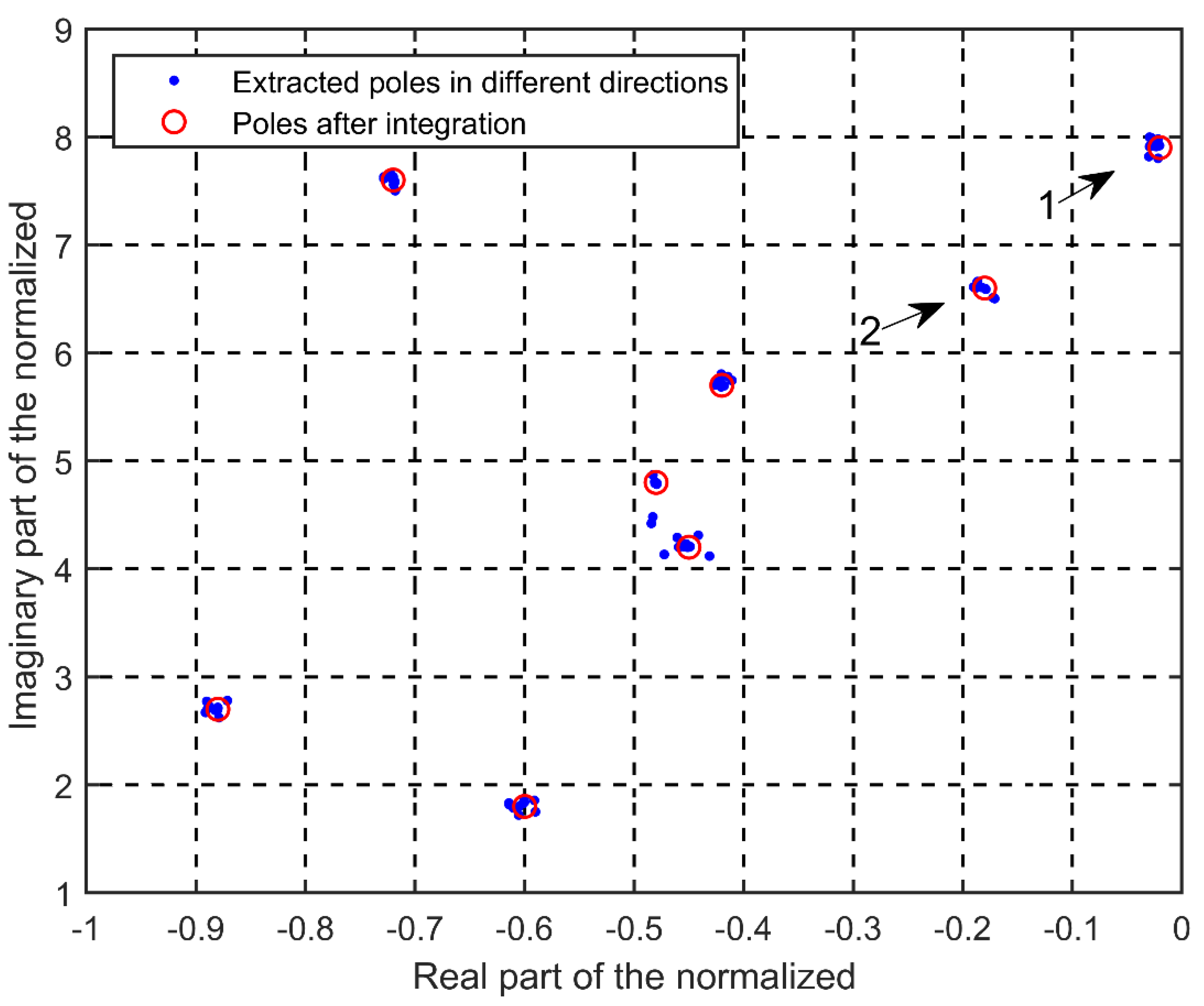
Figure 4 shows the pole results based on the matrix beam method. Figure 5 shows the extracted poles distribution of the ship in ten directions using the method described in this study. Compared with Figure 4 and Figure 5, it is obvious that the method presented herein has two advantages. In Figure 5, the pole locations extracted from different directions are more tightly grouped, which shows that the poles extracted by this method are true poles and exhibit a more distinct aggregation pattern than the poles in Figure 4. This indicates that the poles extraction method in this study has been greatly improved in precision. This is because the matrix beam method only intercepts the late response of the echo data for processing. It can neither avoid the aliasing influence of the early-and late-time responses, nor eliminate the truncation error caused by the late response, thus resulting in large deviations of the poles in different azimuths. Conversely, the poles extraction method proposed in this study was combined with the early-and late-time responses for approximation purposes. Thus, these two defects were overcome, and more efficient and accurate results can be obtained. Moreover, as shown in Figure 5, there are two more poles (poles 1 and 2) compared with those in Figure 4, which demonstrates that the poles extracted by this method are more comprehensive. The omission of true poles in the literature largely lies in the fact that the selected value of the parameters of poles in the matrix beam method is not accurate enough. The method in this study combines the model orders of the system with the specific particle swarm optimization algorithm, and the parameters are greatly optimized, which solves the error problem caused by parameter dependence and avoids the omission of true poles.
4. Conclusions
Feature extraction of complex radar targets plays an important role in applications such as sea and air detection, early warning and modern radar systems. In this study, a set of procedures was designed to accurately extract the pole feature distribution of complex radar targets in the HF band. First, the ARMA model is used to reasonably approximate the entire scattered echo of a complex radar target, it solves the problem of early-and late-time responses aliasing and eliminates the ambiguities generated in traditional late-time methods, to ensure that the possible pole feature information can be extracted effectively. The second, the special particle swarm optimization algorithm combining opposition-based learning and decreasing inertial weights is used to optimize the estimation of model parameters, it effectively solves the problem of parameter dependence in the model algorithm and greatly improves the accuracy of pole extraction. Finally, the sliding window multidirectional correction method is applied to process the initial pole distribution of the complex plane, which makes the corrected multi-directional pole distribution show more distinct aggregation characteristics and better comprehensiveness. This method was tested on the HF radar target of the large complex ship. After a lot of repeated qualitative research, our experiments confirm that the pole features extracted from the targets’ scattering echoes obtain absolute advantages in accuracy, effectiveness and integrity over the reference matrix beam method. It demonstrates the successful performance of the pole feature extraction technology and provides a theoretical basis for complex radar target recognition methods based on pole features in engineering practice.
To maximize the accuracy of pole extraction, the method in this paper selects as many transmission frequencies as possible. However, in the actual pole feature extraction process, the more frequencies are selected, it will take longer time to detect the targets. Therefore, the frequency of this pole extraction method should be optimized to improve its real-time efficiency in the following research.
Author Contributions
Conceptualization, S.Z.; Data curation, S.Z.; Formal analysis, F.R.; Funding acquisition, H.G.; Methodology, S.Z.; Project administration, H.G.; Writing—original draft, S.Z.; Writing—review & editing, H.G. and F.R. All authors have read and agreed to the published version of the manuscript.
Funding
This research was funded by the National Natural Science Foundation of China (No. 61671333), Natural Science Foundation of Hubei Province (No. 2014CFA093), the Fundamental Research Funds for the Central Universities (No. 2042019K50264, No. 2042019GF0013 and No. 2042020gf0003) and the Fundamental Research Funds for the Wuhan Maritime Communication Research Institute (No. 2017J-13 and No. KCJJ2019-05).
Conflicts of Interest
The authors declare no conflict of interest.
References
- Moffatt, D.; Young, J.; Ksienski, A.; Lin, H.; Rhoads, C. Transient response characteristics in identification and imaging. IEEE Trans. Antennas Propag. 1981, 29, 192–205. [Google Scholar] [CrossRef]
- Yang, J.; Sarkar, T.K. Interpolation/extrapolation of radar cross-section (RCS) data in the frequency domain using the Cauchy method. IEEE Trans. Antennas Propag. 2007, 55, 2844–2851. [Google Scholar] [CrossRef]
- Guo, L.; Lin, Y.; Xue, Z.; Zhang, H. A Two Steps Fast Monostatic Radar Cross Section Simulation Scheme Based on Adaptive Cross Approximation and Singular Value Decomposition. In Proceedings of the IEEE International Symposium on Microwave, Antenna, Propagation, and EMC Technologies (MAPE), Xi’an, China, 24–27 October 2017; pp. 369–373. [Google Scholar]
- Bennett, C.L.; Toomey, J.P. Target Classification with Multiple Frequency Illumination. IEEE Trans. Antennas Propag. 1981, 29, 352–358. [Google Scholar] [CrossRef]
- Li, J.; Jen, L. Extraction of natural frequencies of radar target by L/sup 2/ space optimisation. Electron. Lett. 1994, 30, 2072–2073. [Google Scholar] [CrossRef]
- Trueman, C.W.; Kubina, S.J.; Mishra, S.R.; Larose, C.L. RCS of Small Aircraft at HF Frequencies, Proceedings of the Symposium on Antenna Technology and Applied Electromagnetics [ANTEM 1994], Ottawa, ON, Canada, 3–5 August 1994; IEEE: Piscataway, NJ, USA, 1994; pp. 151–157.
- David, A.; Brousseau, C.; Bourdillon, A. Simulations and measurements of a radar cross section of a Boeing 747–200 in the 20–60 MHz frequency band. Radio Sci 2003, 38, 1–3. [Google Scholar] [CrossRef]
- Chan, Y.T.; Ho, K.C.; Wong, S.K. Aircraft identification from RCS measurement using an orthogonal transform. IEE Proc.—Radar Sonar Navig. 2002, 147, 93–102. [Google Scholar] [CrossRef]
- Barès, C.; Brousseau, C.; Bourdillon, A. in A Multifrequency HF—VHF Radar System for Aircraft identification. In Proceedings of the IEEE International Radar Conference, Arlington, VA, USA, 9–12 May 2006. [Google Scholar]
- Gustavsen, B.; Semlyen, A. A robust approach for system identification in the frequency domain. Power Deliv. IEEE Trans. 2004, 19, 1167–1173. [Google Scholar] [CrossRef] [Green Version]
- Deschrijver, D.; Haegeman, B.; Dhaene, T. Orthonormal Vector Fitting: A Robust Macromodeling Tool for Rational Approximation of Frequency Domain Responses. IEEE Trans. Adv. Packag. 2007, 30, 216–225. [Google Scholar] [CrossRef]
- Kennaugh, E.; Moffatt, D.L.; Wang, N. The K-pulse and response waveforms for nonuniform transmission lines. Antennas Propag. IEEE Trans. 1986, 34, 78–83. [Google Scholar] [CrossRef]
- Fiscante, N.; Addabbo, P.; Clemente, C.; Biondi, F.; Giunta, G.; Orlando, D. A Track-Before-Detect Strategy Based on Sparse Data Processing for Air Surveillance Radar Applications. Remote Sens. 2021, 13, 662. [Google Scholar] [CrossRef]
- Wang, R.; Tian, J.; Wu, F.; Zhang, Z.; Liu, H. PSO/GA Combined with Charge Simulation Method for the Electric Field Under Transmission Lines in 3D Calculation Model. Electronics 2019, 8, 1140. [Google Scholar] [CrossRef] [Green Version]
- Morgan, M.A. Singularity expansion representations of fields and currents in transient scattering. IEEE Trans. Antennas Propag. 1984, 32, 466–473. [Google Scholar] [CrossRef]
- Anand, B.; Aakash, I.; Varrun, V.; Reddy, M.K.; Sathyasai, T.; Devi, M.N. Improvisation of Particle Swarm Optimization Algorithm. In Proceedings of the 2014 International Conference on Signal Processing and Integrated Networks (SPIN), Delhi, India, 20–21 February 2014; pp. 20–24. [Google Scholar]
- Tizhoosh, H.R. Opposition-based learning: A new scheme for machine intelligence. In Proceedings of the International Conference on Computational Intelligence for Modelling, Control and Automation and International Conference on Intelligent Agents, Web Technologies and Internet Commerce (CIMCA-IAWTIC’06), Vienna, Austria, 28–30 November 2005; pp. 695–701. [Google Scholar]
- Kumaresan, R.; Tufts, D.W. Estimating the parameters of exponentially damped sinusoids and pole-zero modeling in noise. IEEE Trans. Acoust. Speech Signal Process. 1982, 30, 833–840. [Google Scholar] [CrossRef] [Green Version]
- Jiao, D.; Xu, S.J.; Wu, X.L. New method for natural frequency extraction. Prog. Natual Sci. 1999, 9, 545–552. [Google Scholar]
Figure 1.
Main experimental process of poles extraction.
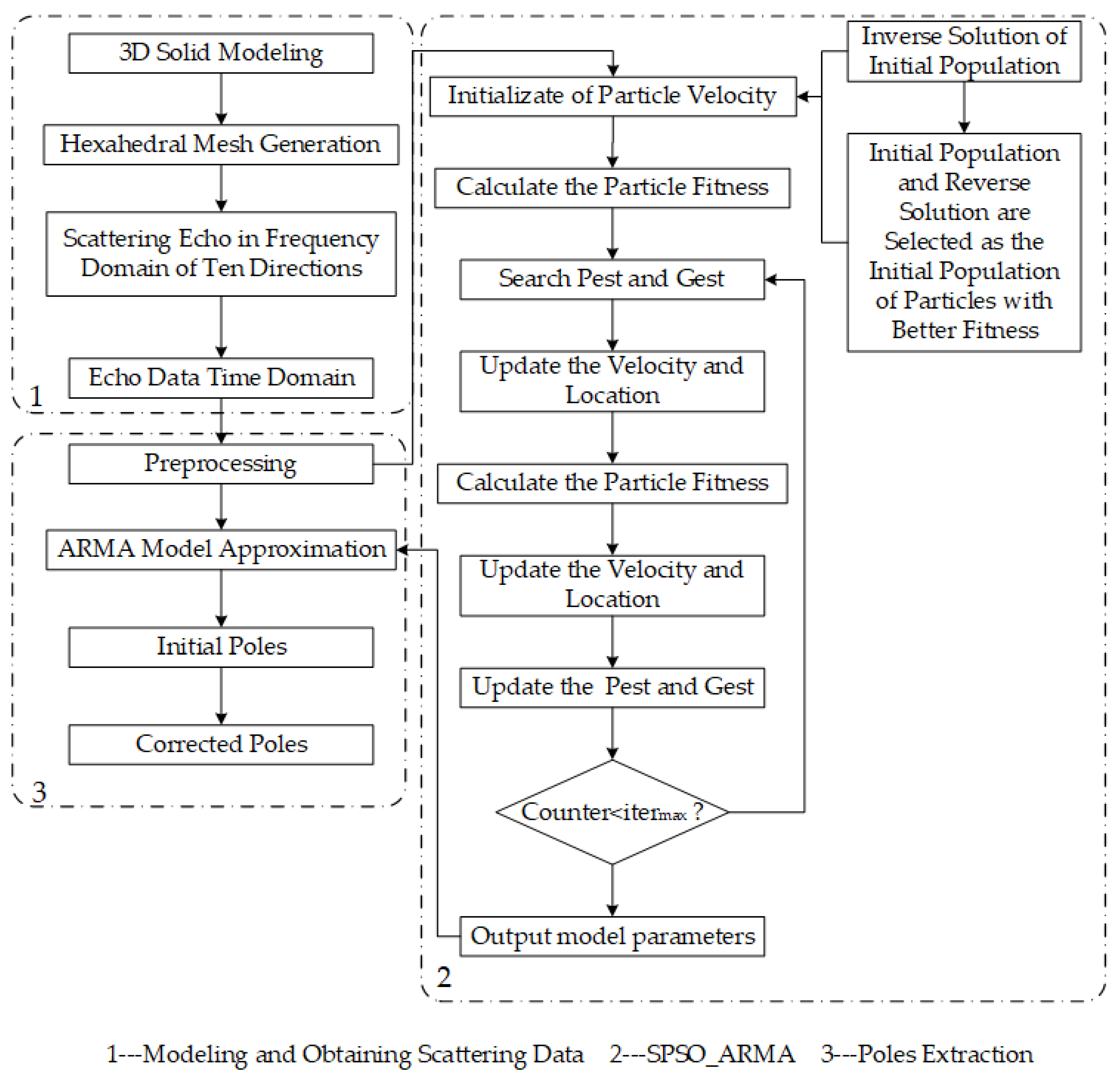
Figure 2.
Hexahedron meshing model of a ship.
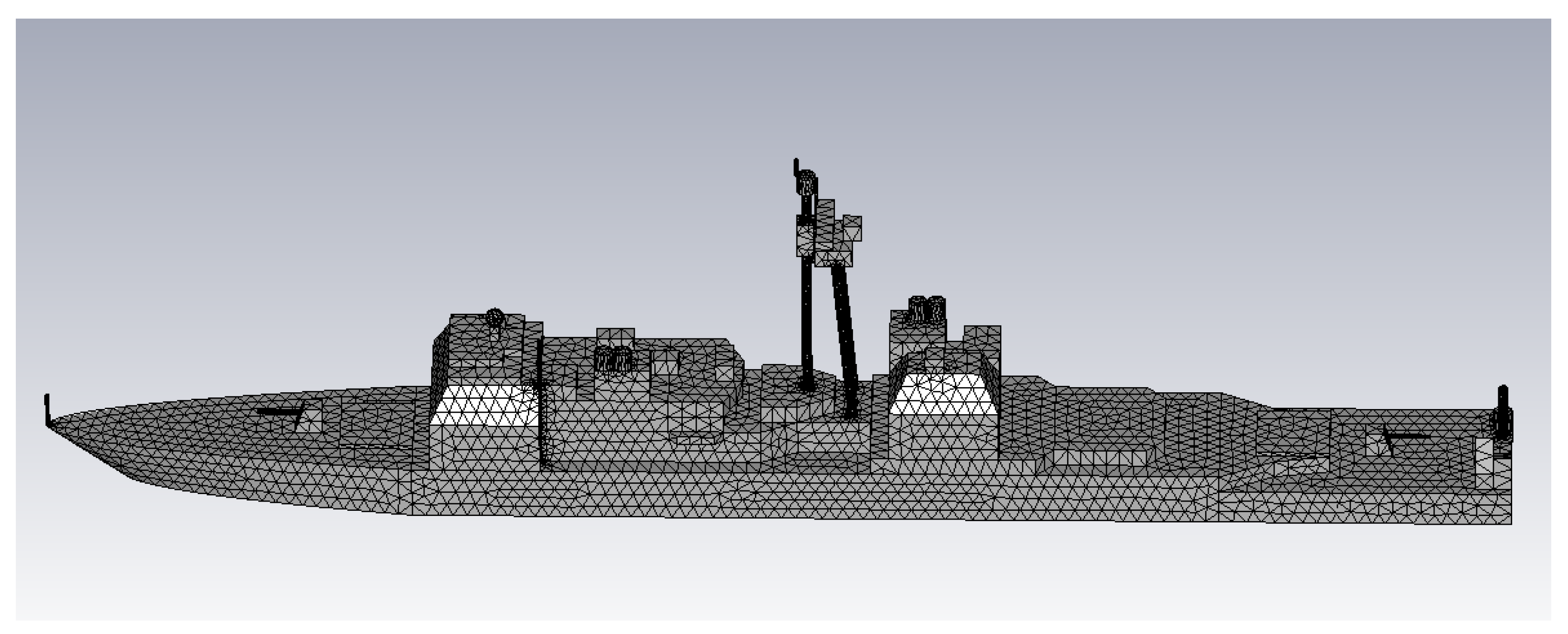
Figure 3.
Scattering data in the frequency domain of the ship target at ten azimuths.
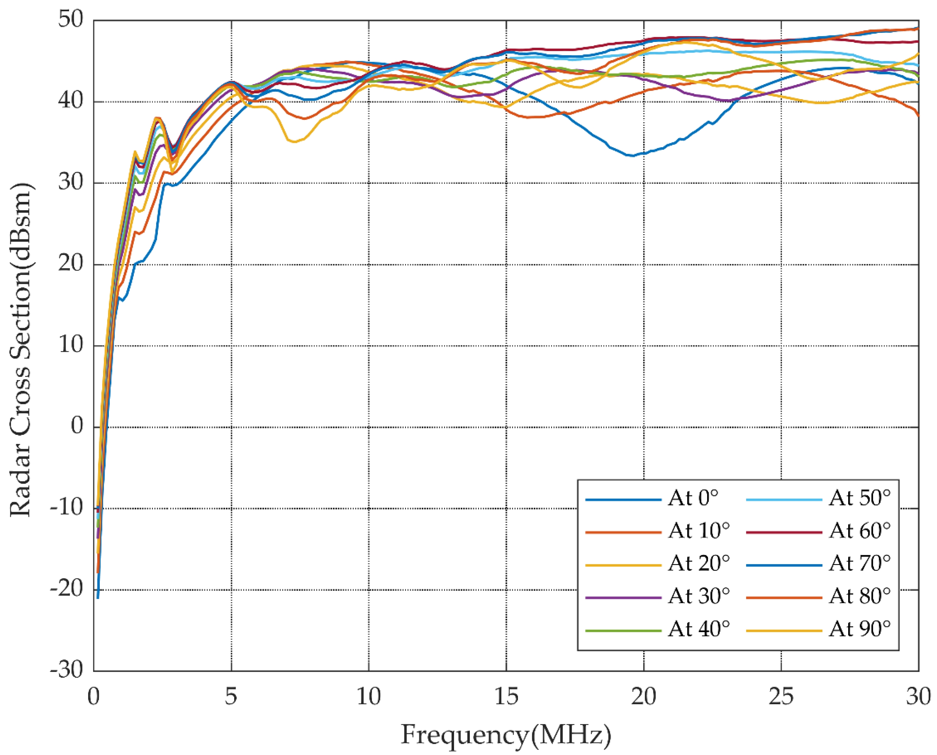
Figure 4.
Extracted poles distribution of the matrix beam method. The blue marks are the original poles extracted in ten directions and the red marks are the poles obtained after correction.
Figure 4.
Extracted poles distribution of the matrix beam method. The blue marks are the original poles extracted in ten directions and the red marks are the poles obtained after correction.
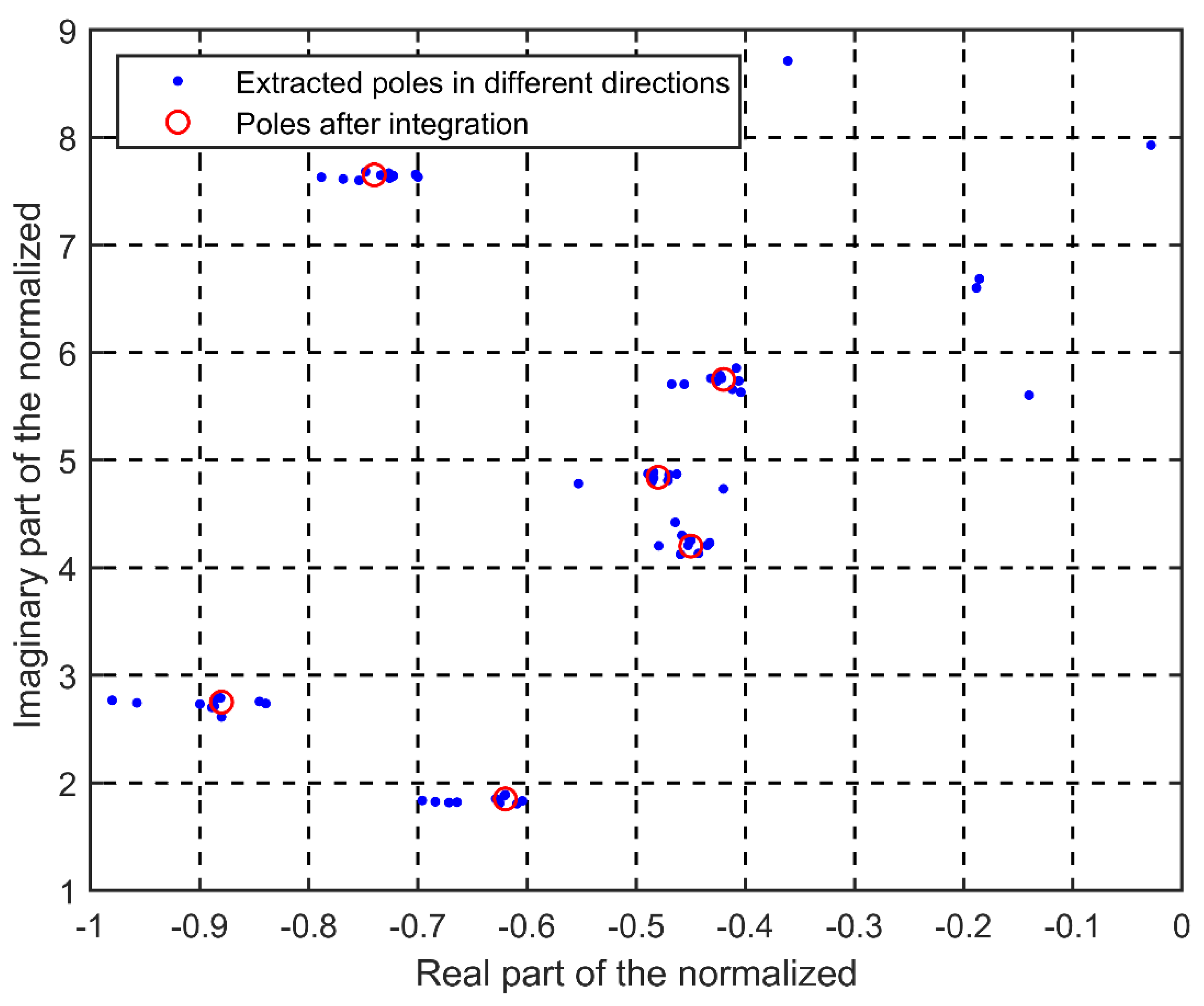
Figure 5.
Extracted poles distribution along ten directions using the method proposed in this study. The blue marks are the original poles extracted in ten directions and the red marks are the poles obtained after correction.
Figure 5.
Extracted poles distribution along ten directions using the method proposed in this study. The blue marks are the original poles extracted in ten directions and the red marks are the poles obtained after correction.
Publisher’s Note: MDPI stays neutral with regard to jurisdictional claims in published maps and institutional affiliations. |
© 2022 by the authors. Licensee MDPI, Basel, Switzerland. This article is an open access article distributed under the terms and conditions of the Creative Commons Attribution (CC BY) license (https://creativecommons.org/licenses/by/4.0/).
Share and Cite
MDPI and ACS Style
Zhou, S.; Gao, H.; Ren, F. Pole Feature Extraction of HF Radar Targets for the Large Complex Ship Based on SPSO and ARMA Model Algorithm. Electronics 2022, 11, 1644. https://doi.org/10.3390/electronics11101644
AMA Style
Zhou S, Gao H, Ren F. Pole Feature Extraction of HF Radar Targets for the Large Complex Ship Based on SPSO and ARMA Model Algorithm. Electronics. 2022; 11(10):1644. https://doi.org/10.3390/electronics11101644
Chicago/Turabian StyleZhou, Sang, Huotao Gao, and Fangyu Ren. 2022. "Pole Feature Extraction of HF Radar Targets for the Large Complex Ship Based on SPSO and ARMA Model Algorithm" Electronics 11, no. 10: 1644. https://doi.org/10.3390/electronics11101644
Note that from the first issue of 2016, this journal uses article numbers instead of page numbers. See further details here.