
Probabilistic Analysis of an RL Circuit Transient Response under Inductor Failure Conditions


Abstract
:1. Introduction
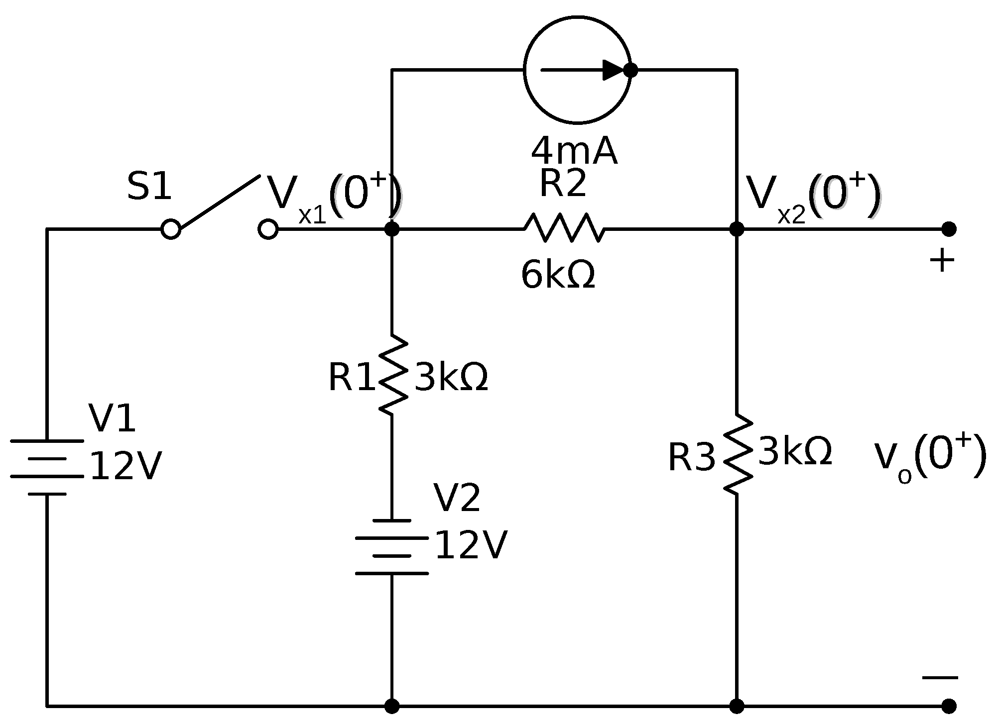
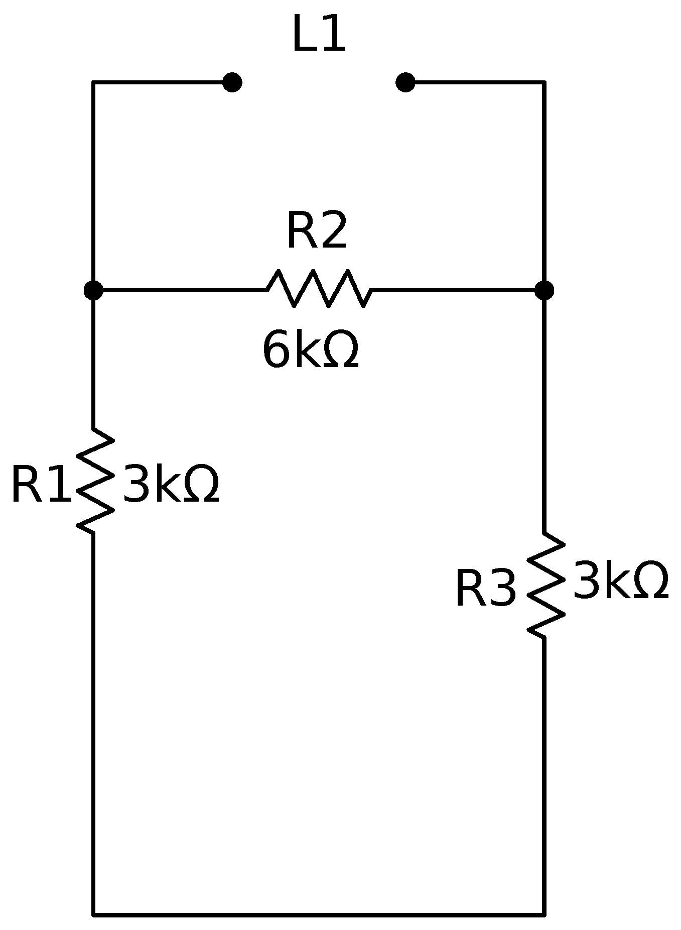
2. RL Circuit Response
2.1. Initial Current through the Inductor
2.2. Initial Voltage at
2.3. Steady State Voltage at
2.4. Time Constant
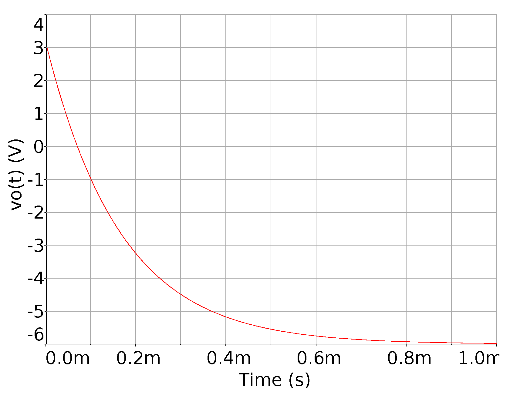
2.5. Circuit Voltage Response
3. Probability Distribution
3.1. Probability Model of
3.1.1.
3.1.2.
3.1.3.
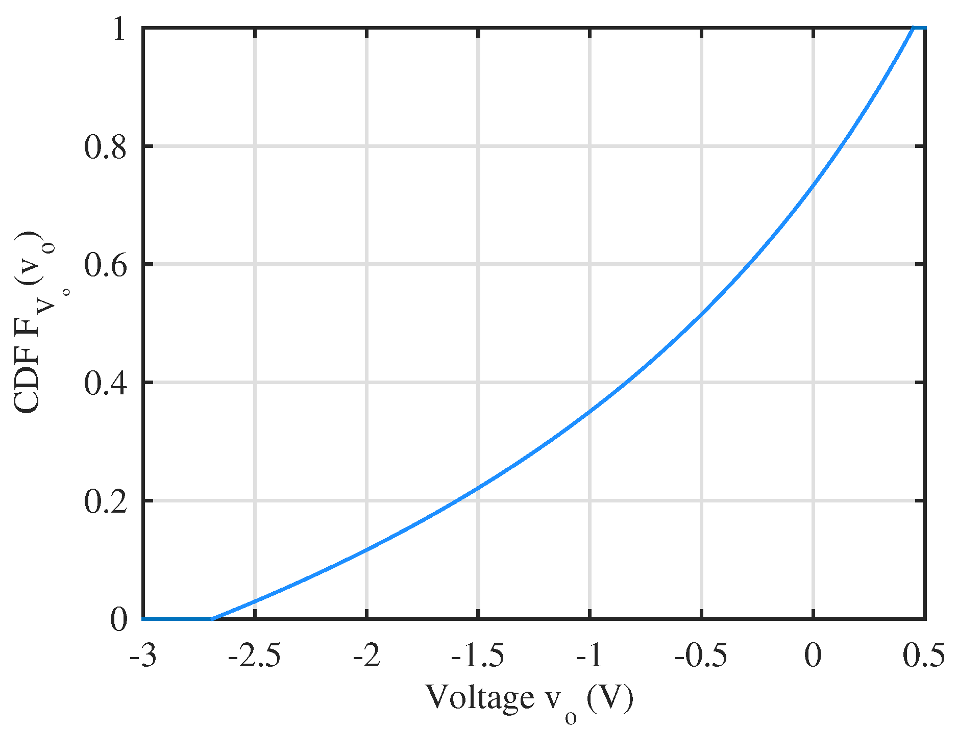
3.1.4. The CDF
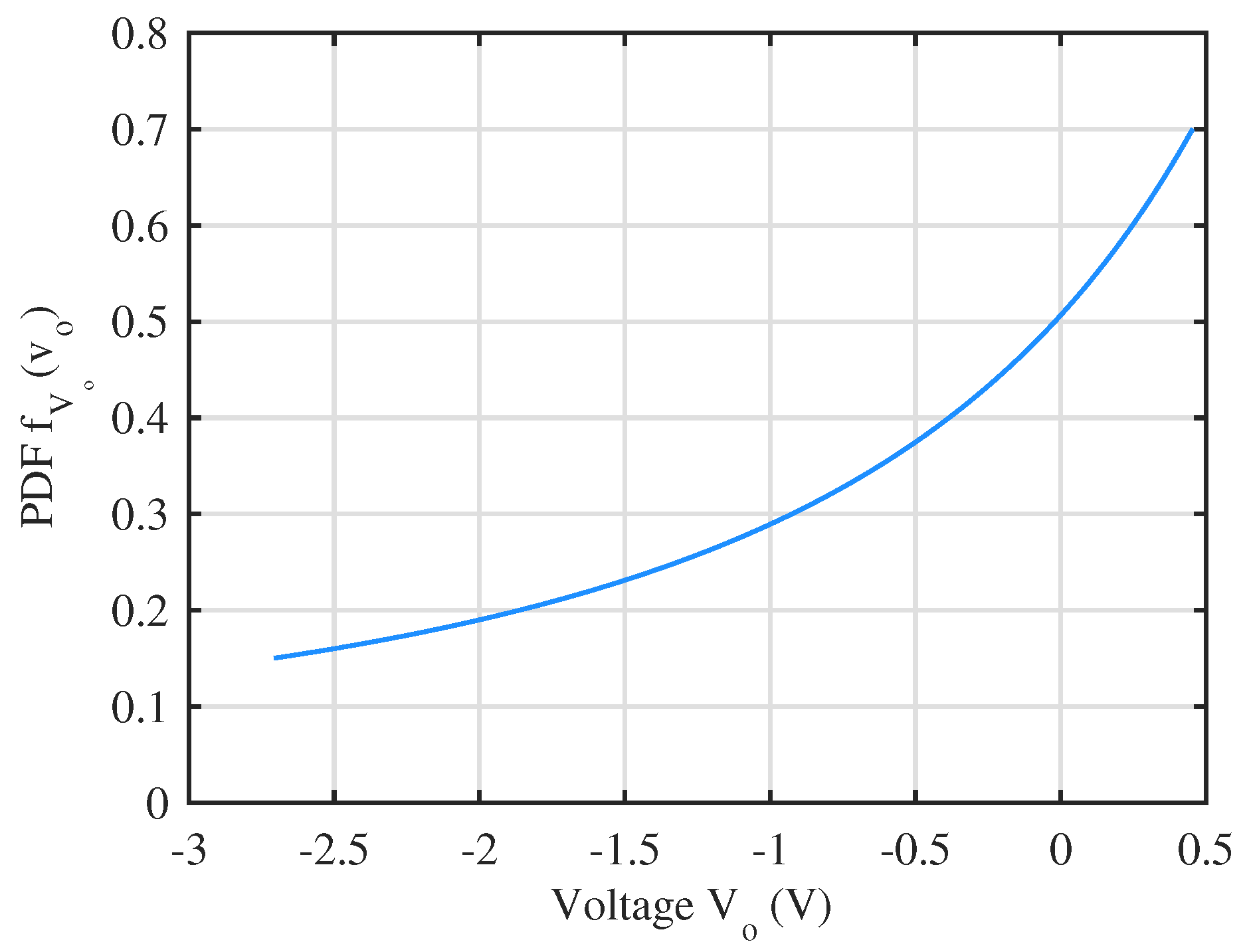
3.1.5. The PDF
3.2. Validity of the Model
3.3. Expected Value
4. Application of the Probability Model
4.1. Examples
4.2. Other Circuit Parameters
4.3. Example for
5. Conclusions
Author Contributions
Funding
Institutional Review Board Statement
Informed Consent Statement
Data Availability Statement
Conflicts of Interest
References
- Gu, Y.; Feng, X.; Chi, R.; Wu, J.; Chen, Y. A Digital Bang-Bang Clock and Data Recovery Circuit Combined with ADC-Based Wireline Receiver. Electronics 2022, 11, 3489. [Google Scholar] [CrossRef]
- Mu, Y.; Hou, N.; Wang, C.; Zhao, Y.; Chen, K.; Chi, Y. An Optoelectronic Detector with High Precision for Compact Grating Encoder Application. Electronics 2022, 11, 3486. [Google Scholar] [CrossRef]
- Ketata, I.; Ouerghemmi, S.; Fakhfakh, A.; Derbel, F. Design and Implementation of Low Noise Amplifier Operating at 868 MHz for Duty Cycled Wake-Up Receiver Front-End. Electronics 2022, 11, 3235. [Google Scholar] [CrossRef]
- Jin, X.Z.; Che, W.W.; Wu, Z.G.; Wang, H. Analog Control Circuit Designs for a Class of Continuous-Time Adaptive Fault-Tolerant Control Systems. IEEE Trans. Cybern. 2020, 52, 4209–4220. [Google Scholar] [CrossRef]
- Sun, J.; Han, G.; Zeng, Z.; Wang, Y. Memristor-Based Neural Network Circuit of Full-Function Pavlov Associative Memory with Time Delay and Variable Learning Rate. IEEE Trans. Cybern. 2020, 50, 2935–2945. [Google Scholar] [CrossRef]
- Liu, L.; Liu, Y.J.; Li, D.; Tong, S.; Wang, Z. Barrier Lyapunov Function-Based Adaptive Fuzzy FTC for Switched Systems and Its Applications to Resistance–Inductance–Capacitance Circuit System. IEEE Trans. Cybern. 2020, 50, 3491–3502. [Google Scholar] [CrossRef]
- Wan, F.; Li, N.; Ravelo, B.; Ji, Q.; Li, B.; Ge, J. The Design Method of the Active Negative Group Delay Circuits Based on a Microwave Amplifier and an RL-Series Network. IEEE Access 2018, 6, 33849–33858. [Google Scholar] [CrossRef]
- Xu, D.; Zhang, W.; Shi, P.; Jiang, B. Model-Free Cooperative Adaptive Sliding-Mode-Constrained-Control for Multiple Linear Induction Traction Systems. IEEE Trans. Cybern. 2020, 50, 4076–4086. [Google Scholar] [CrossRef]
- Lin, Y.S.; Wang, Y.E. Design and Analysis of a 94-GHz CMOS Down-Conversion Mixer With CCPT-RL-Based IF Load. IEEE Trans. Circuits Syst. I Regul. Pap. 2019, 66, 3148–3161. [Google Scholar] [CrossRef]
- Kondo, J.; Tanzawa, T. Pre-Emphasis Pulse Design for Reducing Bit-Line Access Time in NAND Flash Memory. Electronics 2022, 11, 1926. [Google Scholar] [CrossRef]
- Gagliardi, F.; Manfredini, G.; Ria, A.; Piotto, M.; Bruschi, P. Low-Phase-Noise CMOS Relaxation Oscillators for On-Chip Timing of IoT Sensing Platforms. Electronics 2022, 11, 1794. [Google Scholar] [CrossRef]
- Ahmed, O.; Khan, Y.; Butt, M.A.; Kazanskiy, N.L.; Khonina, S.N. Performance Comparison of Silicon- and Gallium-Nitride-Based MOSFETs for a Power-Efficient, DC-to-DC Flyback Converter. Electronics 2022, 11, 1222. [Google Scholar] [CrossRef]
- Sobhan Bhuiyan, M.A.; Hossain, M.R.; Minhad, K.N.; Haque, F.; Hemel, M.S.K.; Md Dawi, O.; Ibne Reaz, M.B.; Ooi, K.J.A. CMOS Low-Dropout Voltage Regulator Design Trends: An Overview. Electronics 2022, 11, 193. [Google Scholar] [CrossRef]
- Ko, J.; Lee, M. A 1.8 V 18.13 MHz Inverter-Based On-Chip RC Oscillator with Flicker Noise Suppression Using Logic Transition Voltage Feedback. Electronics 2019, 8, 1353. [Google Scholar] [CrossRef] [Green Version]
- Wang, Y.; Yu, M.; Ma, K. A Compact Low-Pass Filter Using Dielectric-Filled Capacitor on SISL Platform. IEEE Microw. Wirel. Components Lett. 2021, 31, 21–24. [Google Scholar] [CrossRef]
- Wang, S.F.; Chen, H.P.; Ku, Y.; Zhong, M.X. Analytical Synthesis of High-Pass, Band-Pass and Low-Pass Biquadratic Filters and its Quadrature Oscillator Application Using Current-Feedback Operational Amplifiers. IEEE Access 2021, 9, 13330–13343. [Google Scholar] [CrossRef]
- Yang, M.; Wang, H.; Yang, T.; Hu, B.; Li, H.; Zhou, Y.; Li, T. Design of wide Stopband for Waveguide low-pass Filter Based on Circuit and Field Combined Analysis. IEEE Microw. Wirel. Components Lett. 2021, 31, 1199–1202. [Google Scholar] [CrossRef]
- Şengül, M.; Çakmak, G.; Özdemir, R. Phase Shifting Properties of High-Pass and Low-Pass Mixed-Element Two-Ports. IEEE Trans. Circuits Syst. II Express Briefs 2021, 68, 1208–1212. [Google Scholar] [CrossRef]
- Yutthagowith, P.; Kitcharoen, P.; Kunakorn, A. Systematic Design and Circuit Analysis of Lightning Impulse Voltage Generation on Low-Inductance Loads. Energies 2021, 14, 8010. [Google Scholar] [CrossRef]
- Tuethong, P.; Kitwattana, K.; Yutthagowith, P.; Kunakorn, A. An Algorithm for Circuit Parameter Identification in Lightning Impulse Voltage Generation for Low-Inductance Loads. Energies 2020, 13, 3913. [Google Scholar] [CrossRef]
- Nian, H.; Jin, X. Modeling and Analysis of Transient Reactive Power Characteristics of DFIG Considering Crowbar Circuit under Ultra HVDC Commutation Failure. Energies 2021, 14, 2743. [Google Scholar] [CrossRef]
- Liu, Y.; Zhou, L. Modeling RL Electrical Circuit by Multifactor Uncertain Differential Equation. Symmetry 2021, 13, 2103. [Google Scholar] [CrossRef]
- Xie, L.; Huang, J.; Tan, E.; He, F.; Liu, Z. The Stability Criterion and Stability Analysis of Three-Phase Grid-Connected Rectifier System Based on Gerschgorin Circle Theorem. Electronics 2022, 11, 3270. [Google Scholar] [CrossRef]
- Reverter, F.; Gasulla, M. A Novel General-Purpose Theorem for the Analysis of Linear Circuits. IEEE Trans. Circuits Syst. II Express Briefs 2021, 68, 63–66. [Google Scholar] [CrossRef]
- Barbi, I. A Theorem on Power Superposition in Resistive Networks. IEEE Trans. Circuits Syst. II Express Briefs 2021, 68, 2362–2363. [Google Scholar] [CrossRef]
- Li, Z.; Tang, L.; Liu, J. A Memetic Algorithm Based on Probability Learning for Solving the Multidimensional Knapsack Problem. IEEE Trans. Cybern. 2020, 52, 2284–2299. [Google Scholar] [CrossRef]
- Song, S.; Cheng, M.; He, J.; Zhou, X.; Matsumoto, T. Outage Probability of One-Source-With-One- Helper Sensor Systems in Block Rayleigh Fading Multiple Access Channels. IEEE Sensors J. 2021, 21, 2140–2148. [Google Scholar] [CrossRef]
- Nguyen Duc, H.; Nguyen Hong, N. Optimal Reserve and Energy Scheduling for a Virtual Power Plant Considering Reserve Activation Probability. Appl. Sci. 2021, 11, 9717. [Google Scholar] [CrossRef]
- Li, L.; Huang, Z.; Zhou, J. A Two-Stage Maximum a Posterior Probability Method for Blind Identification of LDPC Codes. IEEE Signal Process. Lett. 2021, 28, 111–115. [Google Scholar] [CrossRef]
- Tan, Y.; Liu, Q.; Liu, J.; Xie, X.; Fei, S. Observer-Based Security Control for Interconnected Semi-Markovian Jump Systems With Unknown Transition Probabilities. IEEE Trans. Cybern. 2021, 52, 9013–9025. [Google Scholar] [CrossRef]
- Hareli, S.; Nave, O.; Gol’dshtein, V. The Evolutions in Time of Probability Density Functions of Polydispersed Fuel Spray—The Continuous Mathematical Model. Appl. Sci. 2021, 11, 9739. [Google Scholar] [CrossRef]
- Sun, L.; Deng, Z. A Fast and Robust Rotation Search and Point Cloud Registration Method for 2D Stitching and 3D Object Localization. Appl. Sci. 2021, 11, 9775. [Google Scholar] [CrossRef]
- Okoth, M.A.; Shang, R.; Jiao, L.; Arshad, J.; Rehman, A.U.; Hamam, H. A Large Scale Evolutionary Algorithm Based on Determinantal Point Processes for Large Scale Multi-Objective Optimization Problems. Electronics 2022, 11, 3317. [Google Scholar] [CrossRef]
- Odeyemi, K.O.; Owolawi, P.A.; Olakanmi, O.O. On Secrecy Performance of a Dual-Hop UAV-Assisted Relaying Network with Randomly Distributed Non-Colluding Eavesdroppers: A Stochastic Geometry Approach. Electronics 2022, 11, 3302. [Google Scholar] [CrossRef]
- Al Mutairi, A. Advanced Approach for Estimating Failure Rate Using Saddlepoint Approximation. Symmetry 2021, 13, 2041. [Google Scholar] [CrossRef]
- Ghahramani, Z. Probabilistic machine learning and artificial intelligence. Nature 2015, 521, 452–459. [Google Scholar] [CrossRef]
- Abdul Majid, A. Forecasting Monthly Wind Energy Using an Alternative Machine Training Method with Curve Fitting and Temporal Error Extraction Algorithm. Energies 2022, 15, 8596. [Google Scholar] [CrossRef]
- Ranftl, S. A Connection between Probability, Physics and Neural Networks. Phys. Sci. Forum 2022, 5, 11. [Google Scholar] [CrossRef]
- Anthony, M. Probability Theory in Machine Learning. In Encyclopedia of the Sciences of Learning; Seel, N.M., Ed.; Springer: Boston, MA, USA, 2012; pp. 2677–2680. [Google Scholar] [CrossRef]


| Symbol | Description |
|---|---|
| a | Minimum value of L |
| b | Maximum value of L |
| Expected value of X | |
| CDF of random variable X | |
| PDF of random variable X | |
| H | Henry |
| Current random variable | |
| Inductor current at | |
| Inductor current just before | |
| Inductor current just after | |
| First constant in circuit response | |
| Second constant in circuit response | |
| L | Inductance random variable |
| l | Arbitrary value of L |
| mA | Milli ampere |
| n | Constant multiplier of |
| Probability of the event | |
| R | Resistance |
| Thevenin equivalent resistance | |
| Set of real numbers | |
| t | Time |
| Time constant | |
| u | Substitution variable |
| V | Volt |
| Voltage random variable | |
| Arbitrary value of random variable | |
| Instantaneous voltage | |
| Voltage at | |
| Voltage at | |
| Voltage at node x |
Publisher’s Note: MDPI stays neutral with regard to jurisdictional claims in published maps and institutional affiliations. |
© 2022 by the authors. Licensee MDPI, Basel, Switzerland. This article is an open access article distributed under the terms and conditions of the Creative Commons Attribution (CC BY) license (https://creativecommons.org/licenses/by/4.0/).
Share and Cite
Farooq-i-Azam, M.; Khan, Z.H.; Hassan, S.R.; Asif, R. Probabilistic Analysis of an RL Circuit Transient Response under Inductor Failure Conditions. Electronics 2022, 11, 4051. https://doi.org/10.3390/electronics11234051
Farooq-i-Azam M, Khan ZH, Hassan SR, Asif R. Probabilistic Analysis of an RL Circuit Transient Response under Inductor Failure Conditions. Electronics. 2022; 11(23):4051. https://doi.org/10.3390/electronics11234051
Chicago/Turabian StyleFarooq-i-Azam, Muhammad, Zeashan Hameed Khan, Syed Raheel Hassan, and Rameez Asif. 2022. "Probabilistic Analysis of an RL Circuit Transient Response under Inductor Failure Conditions" Electronics 11, no. 23: 4051. https://doi.org/10.3390/electronics11234051
APA StyleFarooq-i-Azam, M., Khan, Z. H., Hassan, S. R., & Asif, R. (2022). Probabilistic Analysis of an RL Circuit Transient Response under Inductor Failure Conditions. Electronics, 11(23), 4051. https://doi.org/10.3390/electronics11234051