
Electromagnetic–Thermal Co-Simulation of Planar Monopole Antenna Based on HIE-FDTD Method
1
School of Information and Communications Engineering, Xi’an Jiaotong University, Xi’an 710049, China
2
Shenzhen Research School, Xi’an Jiaotong University, Shenzhen 518057, China
3
National Key Laboratory of Electromagnetic Environment, Qingdao 266107, China
*
Author to whom correspondence should be addressed.
Electronics 2022, 11(24), 4167; https://doi.org/10.3390/electronics11244167
Submission received: 29 October 2022
/
Revised: 5 December 2022
/
Accepted: 12 December 2022
/
Published: 13 December 2022
(This article belongs to the Special Issue Recent Advancements and Applications of Computational Electromagnetics)
Abstract
:This paper presents an efficient approach to implement electromagnetic-thermal (EM-T) co-simulation of a planar monopole antenna based on hybrid implicit-explicit finite-difference time-domain method (HIE-FDTD-M). First, the EM simulation is carried out by solving Maxwell’s curl equation. Once the EM field reaches steady state, the EM power loss is computed according to the electric conductivity of the material. Finally, the thermal field is simulated by taking the EM power loss as the heat source in the heat transfer equation (HTE). For comparison, HIE-FDTD-M and FDTD-M are adopted respectively in the computation of the EM field. The simulated EM parameters of the planar monopole antenna, including S11 and radiation pattern, are consistent with those obtained by using CST software. The thermal field distribution on the surface of the antenna computed by the proposed method in this paper is approximately similar to that obtained using COMSOL software. However, the EM-T co-simulation of the antenna using HIE-FDTD-M takes only 1/11 of the time required using FDTD-M.
1. Introduction
In microwave applications, electromagnetic-thermal (EM-T) co-design has been a significant problem. On the one hand, EM-T co-simulation can avoid mechanical damage of microwave devices caused by electromagnetic (EM) heat. On the other hand, EM-T co-simulation can positively apply EM heat to some scenarios that require environmentally friendly heating. The current research on EM-T coupling in EM field is mainly focused on antenna, metamaterial, and microwave heating. For metamaterials, their EM and thermal performance in a high-power microwave (HPM) environment have gained much attention. Seviour et al. explored the EM-T performance of a metamaterial which was composed of Split Ring Resonators (SRRs) printed on FR-4 in [1]. The research pointed out that when the EM wave with frequency of 10 GHz and power of 1 W irradiated the SRRs for 15 s, part of the SRRs burned down. A detailed EM-T coupling analysis of the cross-slot frequency selective surface (FSS) was performed by Lu et al. in [2]. They found that the temperature rise of the wide-slot FSS was significantly lower than that of the narrow-slot FSS under the same experimental conditions, and the temperature distributions of the FSS changed with the incidence angle of the EM waves. In addition, the investigation of EM-T effects of metamaterial absorber (MA) has also been paid more attention recently. The finite-difference time-domain method (FDTD-M) was utilized to analyze the thermal effect and absorption performance of a radio-wave absorber by Suga et al. in [3]. It was found that the frequency and amplitude of the absorption peak of the absorber varied with temperature. In et al. researched the influences of Joule heat on the absorbing efficiency of MA in [4]. Lv et al. proposed that the frequency of incident EM wave and the sheet resistance of graphene were both factors affecting the EM-T effects of graphene-based MA [5]. In addition, thermally tunable and thermally stable water-based absorbers have become a hot research topic in recent years [6,7,8,9]. For microwave heating, it has a wide range of applications in the fields of biomedical therapy, preparation of chemical materials, industrial sintering, etc. For example, microwave ablation technique can heat the tumor cells to coagulate and necrotize by using antenna probes without affecting the surrounding healthy tissue [10,11,12], and microwave thermotherapy is effective in improving microenvironment, increasing microcirculation, promoting the absorption of necrotic material, and accelerating recovery [13].
As a transition device between the guiding wave system and free space, the antenna is widely used in wireless communication, satellite navigation, radar system, electronic countermeasures, and many other EM fields [14,15]. A huge number of articles on antenna design have been published since the antenna was proposed. Most studies focus on improving the EM performance of the antenna, such as broadening the bandwidth, increasing the gain, reshaping the radiation pattern [16,17], etc. However, with the expansion of antenna applications, EM-T co-design of the antenna needs to be considered under some circumstances. For an active phased array antenna (APAA), the heat generated by its transmit/receive module (TRM) and power source can cause structural distortion of the array plane and then affect the electrical performance of the antenna [18,19]. In addition, the high-power devices in microwave wireless power transmission system also produce a significant amount of thermal power, which will also affect the EM performance of the antenna [20]. For space-borne antennas, they have to undergo long-term solar irradiation and low temperature heat sink effect in space, so the thermodynamic and mechanical properties of their materials will be significantly decreased, which will eventually affect their electrical properties [21,22,23,24]. The existing study on EM-T co-simulation of antenna is mainly devoted to analyzing the effects of external temperature variation on the structure deformation and radiation characteristics of antenna. In fact, the EM power loss of the antenna itself can also cause significant temperature rise, which will lead to antenna performance degradation. However, the research on the EM-T coupling field analysis of antenna is relatively little [25].
The FDTD-M is often employed in the simulations of EM and thermal fields [26,27,28]. However, the FDTD-M has the disadvantage of low computational efficiency when simulating EM problems with fine structures. Some unconditionally stable [29,30] and weakly conditionally stable FDTD methods [31,32] are proposed to solve this issue. Among them, the hybrid implicit-explicit FDTD-M (HIE-FDTD-M) is extremely appropriate for simulating EM problems which have very small grid size in one dimension. A previous study demonstrated that the calculation efficiency of HIE-FDTD-M is higher than that of FDTD-M, and the calculation accuracy exceeds that of alternating-direction implicit FDTD-M for one-dimensional mini-lattice problem [33]. Although the HIE-FDTD-M has a wide range of applications in solving one-dimensional fine structure EM problems, such as graphene-based EM devices [34], microstrip circuits, antennas [35,36], etc., no study has been carried out to apply the HIE-FDTD-M to antenna EM-T co-simulation. In addition, most studies on HIE-FDTD-M in linear, non-dispersive space do not consider dielectric losses. However, when the HIE-FDTD-M is extended to EM-T co-simulation, there must be lossy medium in the simulation target. At this time, the iteration coefficients in the calculating equations of EM components and the final expressions of the implicit EM components in the HIE-FDTD-M are different from those in lossless media. Unno et al. investigated the HIE-FDTD-M containing lumped elements and conductive media in [36], but they did not consider absorption boundary condition. Therefore, this study is only applicable to the calculation of closed region problems and not to the computation of open area problems, such as antennas.
In this paper, we extend the HIE-FDTD-M to the EM-T coupling field analysis of a planar monopole antenna. Using HIE-FDTD-M instead of FDTD-M to calculate EM fields can shorten the EM-T co-simulation time of the antenna by 11 times, which well proves the high efficiency of the proposed method. In addition, the simulation results of the antenna obtained by the presented method are consistent with those obtained by commercial software CST and COMSOL, which verifies the correctness of the proposed method. The simulation results demonstrate the feasibility of HIE-FDTD-M in computing one-dimensional fine structure EM-T problems, especially those with thin layer structures.
2. Methods and Formulations
The calculation process of the EM-T co-simulation is shown in Figure 1. Firstly, the EM field is simulated until it reaches steady state. Then the EM power loss is calculated according to the electric fields and the material properties. Finally, the EM power loss serves as the heat source in HTE, and the thermal field is simulated.
2.1. HIE-FDTD Method for Solving EM Field
The EM field is simulated by solving Maxwell’s curl equations
In linear, isotropic, and nondispersive media, the discretization formulas of Maxwell’s curl equations based on HIE-FDTD-M in y direction [33] are
where , , , ; ε—permittivity (F/m), σ—conductivity (S/m), μ—permeability (H/m), σm—equivalent magnetic loss (Ω/m); n represents the time sampling point, and Δt represents the time duration between two adjacent time sampling points; Δx, Δy, and Δz represent the three-dimensional size of the Yee cell, and m, p, and q indicate the position of the Yee cell. In addition, the convolutional perfectly matched layer (CPML) approach is employed in Equation (2) to truncate the calculation area. The calculation formulas of κ and Ψ which are related to CPML in Equation (2) are given in Appendix A.
The and in right sides of Equations (2-1) and (2-3) are unknown quantities. Substituting Equation (2-6) into Equation (2-1), the final calculation formula of is simplify to
where , , , , .
Substituting Equation (2-4) into Equation (2-3), the final calculation formula of is simplified to
where , .
In HIE-FDTD-M, the components of the EM field need to be updated sequentially. Firstly, compute according to Equation (2-2). Then update and based on Equations (3) and (4) by solving tridiagonal matrices. Finally, update , and according to the electric field values at the new moment.
For Equation (2), the time step size (TSS) needs to satisfy the following expressions [33]
Equation (5) indicates that the TSS of HIE-FDTD-M is independent of the mesh size in y direction. Therefore, when the Δy of the EM problem is much smaller than Δx and Δz, the TSS of HIE-FDTD-M can be set much bigger than that of FDTD-M.
2.2. EM Power Loss and Thermal Field Calculation
When some media are exposed to the EM environment, EM energy in the media can be converted into heat energy due to the displacement of electrons, electric polarization, and magnetic polarization, etc. The dissipated EM energy can be obtained by calculating EM power loss. Because of the different ways in which EM energy is dissipated, the expressions of EM power loss are different. In [27], a microwave heating process of phantom food gel was simulated by using the FDTD model. The calculation formula of EM power loss and the conversion relation between the EM field and the thermal field were given in this paper. In [28], the FDTD method is extended to the EM-T coupling analysis of frequency-dependent and temperature-dependent media. The complex Debye permittivity was analyzed, and the transient EM power loss was derived.
In this paper, we only consider the EM power loss caused by dielectric conductivity. When the excitation signal of the EM field is sinusoidal, the EM power loss can be calculated by the following expression:
where E is the electric field value at the thermal field node.
Since the EM field is a vector, and the thermal field is a scalar, the EM field node and the thermal field node cannot coincide exactly. In this paper, the thermal field node is located at the geometric center of the grid. The spatial distributions of the thermal field node and EM field components are shown in Figure 2. As shown in Figure 2, the components of the EM field are distributed on the edges of Yee cell. The electric field at the center of the Yee cell can be calculated by linear interpolation of the electric fields at the edges, as expressed in Equation (7).
where Ex, Ey, and Ez can be obtained by looking for the maximum values of the corresponding electric field components after the EM field reaches the steady state.
The thermal field is calculated based on HTE
where ρ—medium density (kg/m3); Cm—specific heat of the medium (J/(kg·K)); T—medium temperature (K); kt—thermal conductivity (W/(m·K)); P—heat flux density (W/m3). When ρ, Cm, and kt do not change with position, temperature, and time, HTE can be simplified as
where .
The discretization formula of Equation (9) is
where Δxh, Δyh, and Δzh are the distances between two thermal field nodes. Δth is the TSS of thermal field simulation. In addition, the heat source P in Equation (10) is equal to the EM power loss.
The time stability condition of Equation (10) is
In addition to Equation (9), the convective boundary conditions are used at the surface of the antenna, which can be written as
where h—convection heat transfer parameter (W/(m2·K)); p—unit vector normal to the surface of the antenna; Tsurf—surface temperature of the antenna (K); Text—ambient temperature (K).
3. Model and Results
The structure and dimensions of the planar monopole antenna are given in Figure 3. As shown in Figure 3a, the antenna consists of three parts, which are monopole patch, dielectric substrate, and ground. The monopole patch and ground are made of metal, and the dielectric substrate is made of lossy FR4. The thickness of the dielectric substrate is 0.2 mm. The EM and thermal parameters of the substrate are εr = 4.5, μr = 1, σ = 0.004, σm = 0, ρ = 1900, kt = 0.3, and Cp = 1369.
In the EM-thermal co-simulation of the antenna, we need not only to analyze the thermal effect of the antenna but also to pay attention to its EM characteristics. Therefore, we first simulate the EM performance of the antenna, including the simulations of S parameter and radiation patterns. The S11 of the planar monopole antenna is simulated by adopting HIE-FDTD-M, FDTD-M and CST software, respectively, and the corresponding results are given in Figure 4. As shown in Figure 4, the working frequency of the planar monopole antenna is 2.38 GHz. The S11 calculated using HIE-FDTD-M is consistent with those calculated using the FDTD-M and CST software.
Figure 5 illustrates the radiation patterns of the planar monopole antenna. As shown in Figure 5, the directivity pattern curves calculated by the three approaches present good consistency.
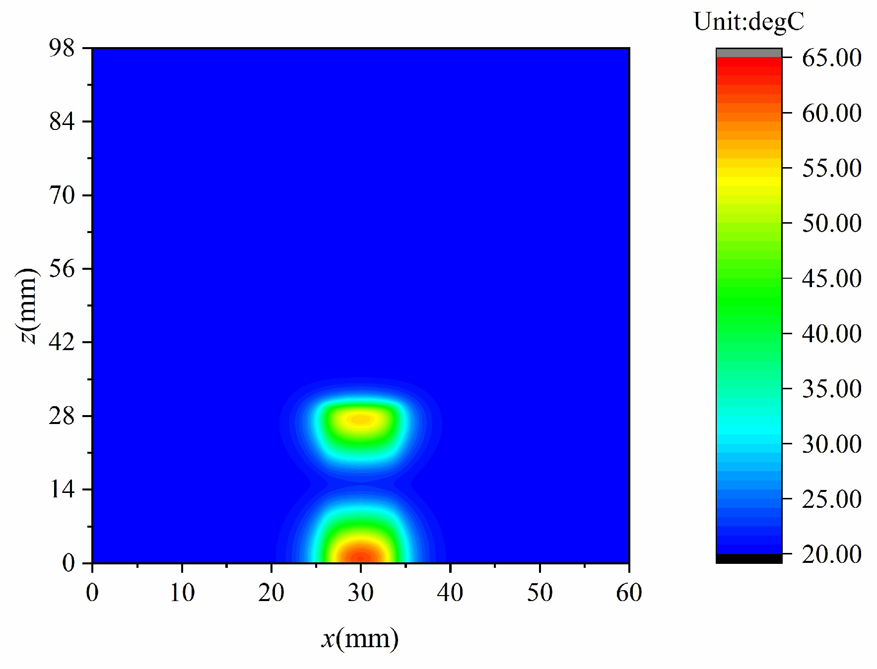
After ensuring that the antenna can work normally, the thermal field of the antenna is simulated. For comparison, the HIE-FDTD-M and the traditional FDTD-M are utilized to calculate the EM field respectively until the EM field reaches the steady state. Then the EM power loss is calculated according to the steady-state electric field and material conductivity. Finally, the EM power loss is used as the heat source in HTE to calculate the thermal field. Assume that the initial temperature of the antenna and its ambient environment is 20 °C, and the convection heat transfer parameter h = 5. The antenna is driven by a voltage source. The signal of the voltage source is a sine wave with frequency of 2.38 GHz. The magnitude of the signal is 10 V/m. The thermal field distributions on the surface of the dielectric substrate after 300 s are shown in Figure 6. The thermal field distributions in Figure 6a,b are completely consistent, and the maximum temperature in both figures is 64.2 °C. In addition, the same antenna model is simulated by using multi-physical simulation software COMSOL Multiphysics and the result are shown in Figure 7. The maximum temperature in Figure 7 is 61.8 °C. We can find that the thermal field distribution calculated by the EM-thermal coupling method proposed in this paper matches well with that by using COMSOL software, and the maximum temperature difference is only 2.4 °C.
4. Discussion
According to the time stability condition, the TSSs of the HIE-FDTD-M and FDTD-M are, respectively, 3.77 ps and 0.27 ps. The EM field reaches the steady state after 18 ns. Therefore, the time step numbers needed for EM field simulation with HIE-FDTD-M and conventional FDTD-M are, respectively, 5000 and 68,120. The times consumed for the EM field simulation by these two approaches are, respectively, 15.5 min and 172.1 min. On the basis of Equations (5) and (10), Δt is much smaller than Δth. Generally, Δth is on the order of seconds while Δt is on the order of picoseconds. In this example, the TSS of thermal field simulation is 0.388 s. When the simulation time of the thermal field is 300 s, the required time is only 5s, which can be almost ignored compared with the EM field simulation time. The total required time for EM-T co-simulation of HIE-FDTD-M is only 1/11 of that of the FDTD-M. The above data are completed on a PC with Intel Core i7-12700F of 2.1 GHz and RAM of 32 GB.
The simulation results show that the HIE-FDTD-M is very suitable for EM-thermal coupling simulation of antennas with fine structures in one direction, especially those with thin layer structures.
5. Conclusions
The HIE-FDTD-M is applied to EM-thermal co-simulation of planar monopole antenna in this article. When the simulation model has one-dimensional mini-lattice, the adoption of HIE-FDTD-M can avoid the influence of the small grid size on the TSS. At this time, the simulation speed of HIE-FDTD-M is much faster than that of FDTD-M. In EM-T co-simulation, the simulation time of the EM field is much longer than that of the thermal field, so the HIE-FDTD-M also shows high efficiency in the EM-T co-simulation of one-dimensional fine problems. In the numerical example of the planar monopole antenna, the time consumed in EM-T co-simulation using HIE-FDTD-M is only 1/11 of that using FDTD-M. Simulation results show that the HIE-FDTD-M is very suitable for the EM-T co-simulation of EM problems with one-dimensional fine structure, especially those with thin layer structures.
Author Contributions
Conceptualization, C.M. and J.C.; methodology, C.M. and H.P.; writing, software, and data curation, C.M. All authors have read and agreed to the published version of the manuscript.
Funding
This research was supported by the National Natural Science Foundations of China (No. 61971340); by the Technology Program of Shenzhen (grant number JCYJ20180508152233431); and also by the National Key Laboratory of Electromagnetic Environment (grant number 202102011).
Institutional Review Board Statement
Not applicable.
Informed Consent Statement
Not applicable.
Data Availability Statement
Not applicable.
Conflicts of Interest
The authors declare no conflict of interest.
Appendix A
References
- Seviour, R.; Tan, Y.S.; Hopper, A. Effects of High Power on Microwave Metamaterials. In Proceedings of the 8th International Congress on Advanced Electromagnetic Materials in Microwaves and Optics-Metamaterials, Copenhagen, Denmark, 25–30 August 2014. [Google Scholar]
- Lu, Y.; Chen, J.; Li, J.X.; Xu, W.J. A Study on the Electromagnetic–Thermal Coupling Effect of Cross-Slot Frequency Selective Surface. Materials 2022, 15, 640. [Google Scholar] [CrossRef] [PubMed]
- Suga, R.; Hashimoto, O.; Pokharel, R.K.; Wada, K.; Watanabe, S. Analytical Study on Change of Temperature and Absorption Characteristics of a Single-Layer Radiowave Absorber Under Irradiation Electric Power. IEEE Trans. Electromagn. Compat. 2005, 47, 866–871. [Google Scholar] [CrossRef]
- In, S.; Park, N. Effects of Optical Joule Heating in Metamaterial Absorber: A Non-Linear Recursive Feedback Optical-Thermodynamic Multiphysics Study. In Proceedings of the 9th International Congress on Advanced Electromagnetic Materials in Microwaves and Optics–Metamaterials, Oxford, UK, 7–12 September 2015. [Google Scholar]
- Lv, W.Q.; Lu, W.B. Electromagnetic Heating Effect of Graphene Absorber. In Proceedings of the 2019 International Applied Computational Electromagnetics Society Symposium-China (ACES), Nanjing, China, 8–11 August 2019. [Google Scholar]
- Yan, X.X.; Kong, X.K.; Wang, Q.; Xing, L.; Xue, F.; Xu, Y.; Jiang, S.L.; Liu, X.C. Water-Based Reconfigurable Frequency Selective Rasorber with Thermally Tunable Absorption Band. IEEE Trans. Antennas Propag. 2020, 68, 6162–6171. [Google Scholar] [CrossRef] [Green Version]
- Li, S.R.; Shen, Z.Y.; Yang, H.L.; Liu, Y.J.; Hua, L.N. Ultra-Wideband Transmissive Water-Based Metamaterial Absorber with Wide Angle Incidence and Polarization Insensitivity. Plasmonics 2021, 16, 1269–1275. [Google Scholar] [CrossRef]
- Zhang, X.F.; Zhang, D.J.; Fu, Y.J.; Li, S.H.; Wei, Y.; Chen, K.J.; Wang, X.; Zhuang, S.L. 3-D Printed Swastika-Shaped Ultrabroadband Water-Based Microwave Absorber. IEEE Antennas Wirel. Propag. Lett. 2020, 19, 821–825. [Google Scholar] [CrossRef]
- Xie, J.W.; Quader, S.; Xiao, F.J.; He, C.; Liang, X.L.; Geng, J.P.; Jin, R.H.; Zhu, W.R.; Rukhlenko, I.D. Truly All-Dielectric Ultrabroadband Metamaterial Absorber: Water-Based and Ground-Free. IEEE Antennas Wirel. Propag. Lett. 2019, 18, 536–540. [Google Scholar] [CrossRef]
- Palandoken, M.; Murat, C.; Kaya, A.; Zhang, B. A Novel 3-D Printed Microwave Probe for ISM Band Ablation Systems of Breast Cancer Treatment Applications. IEEE Trans. Microw. Theory Tech. 2022, 70, 1943–1953. [Google Scholar] [CrossRef]
- Lin, S.; Chen, H.D.; Che, W.Q.; Xue, Q. Experiments of Microwave Ablation Based on Dual-Frequency Antenna under Pulsed Mode. IEEE Antennas Wirel. Propag. Lett. 2022, 21, 848–852. [Google Scholar] [CrossRef]
- Chen, H.D.; Lin, S.; Che, W.Q.; Xue, Q. Study of Single- and Dual-Frequency Microwave Ablation Antennas Based on Shorted Helical Slot. IEEE Trans. Antennas Propag. 2022, 70, 598–606. [Google Scholar] [CrossRef]
- Lin, S.J.; Chen, H.C.; Chiu, H.W. CMOS Monolithic Thermostatic Microwave Heater with Bioimpedance Load Effect Compensation. IEEE Trans. Microw. Theory Tech. 2022, 70, 5271–5277. [Google Scholar] [CrossRef]
- Song, W.L.; Weng, Z.B.; Jiao, Y.C.; Wang, L.; Yu, H.W. Omnidirectional WLAN Antenna with Common-Mode Current Suppression. IEEE Trans. Antennas Propag. 2021, 69, 5980–5985. [Google Scholar] [CrossRef]
- Falkner, B.J.; Zhou, H.Y.; Mehta, A.; Arampatzis, T.; Dariush, M.S.; Nakano, H. A Circularly Polarized Low-Cost Flat Panel Antenna Array with a High Impedance Surface Meta-Substrate for Satellite On-the-Move Medical IoT Applications. IEEE Trans. Antennas Propag. 2021, 69, 6076–6081. [Google Scholar] [CrossRef]
- Qin, D.J.; Sun, B.H.; Zhang, R. VHF/UHF Ultrawideband Slim Monopole Antenna with Parasitic Loadings. IEEE Antennas Wirel. Propag. Lett. 2022, 21, 2050–2054. [Google Scholar] [CrossRef]
- Leszkowska, L.; Rzymowski, M.; Nyka, K.; Kulas, L. High-Gain Compact Circularly Polarized X-Band Superstrate Antenna for CubeSat Applications. IEEE Antennas Wirel. Propag. Lett. 2021, 20, 2090–2094. [Google Scholar] [CrossRef]
- Wang, C.S.; Duan, B.Y.; Zhang, F.S.; Zhu, M.B. Coupled Structural–Electromagnetic–Thermal Modelling and Analysis of Active Phased Array Antennas. Microw. Antennas Propag. 2020, 4, 247–257. [Google Scholar] [CrossRef]
- Wang, Y.; Wang, C.S.; Lian, P.Y.; Xue, S.; Liu, J.; Gao, W.; Shi, Y.; Wang, Z.H.; Yu, K.P.; Peng, X.L.; et al. Effect of Temperature on Electromagnetic Performance of Active Phased Array Antenna. Electronics 2022, 9, 1211. [Google Scholar] [CrossRef]
- Qian, S.H.; Duan, B.Y.; Lou, S.X.; Ge, C.L.; Wang, W. Investigation of the Performance of Antenna Array for Microwave Wireless Power Transmission Considering the Thermal Effect. IEEE Antennas Wirel. Propag. Lett. 2022, 21, 590–594. [Google Scholar] [CrossRef]
- Zhu, M.B.; Zhong, Y.F.; Duan, B.Y. Multiply Factors Simulation Analysis for Thermal Deformation of Space-borne Antenna. J. Syst. Simul. 2007, 19, 1376–1378. [Google Scholar]
- Takahashi, T.; Nakamoto, N.; Ohtsuka, M.; Aoki, T.; Konishi, Y.; Chiba, I.; Yajima, M. On-Board Calibration Methods for Mechanical Distortions of Satellite Phased Array Antennas. IEEE Trans. Antennas Propag. 2012, 60, 1362–1372. [Google Scholar] [CrossRef]
- Liu, Y.T.; Zhang, S.Y.; Gao, Y.G. A High-Temperature Stable Antenna Array for the Satellite Navigation System. IEEE Antennas Wirel. Propag. Lett. 2017, 16, 1397–1400. [Google Scholar] [CrossRef]
- Chen, J.; Zhou, Y.Q. Ambiguity Performance Analysis of Spaceborne SAR with Thermal Mechanism Errors in Phased Array Antenna. J. Beijing Univ. Aeronaut. Astronaut. 2004, 30, 839–843. [Google Scholar]
- Zhang, H.X.; Huang, L.; Wang, W.J.; Zhao, Z.G.; Zhou, L.; Chen, W.C.; Zhou, H.J.; Zhan, Q.W.; Kolundzija, B.; Yin, W.Y. Massively Parallel Electromagnetic–Thermal Cosimulation of Large Antenna Arrays. IEEE Antennas Wirel. Propag. Lett. 2020, 19, 1551–1555. [Google Scholar] [CrossRef]
- Lu, Y.L.; Ying, J.L.; Tan, T.-K.; Arichandran, K. Electromagnetic and Thermal Simulations of 3-D Human Head Model under RF Radiation by Using the FDTD and FD Approaches. IEEE Trans. Magn. 1996, 32, 1653–1656. [Google Scholar]
- Ma, L.Z.; Paul, D.-L.; Pothecary, N.; Railton, C.; Bows, J.; Barratt, L.; Mullin, J.; Simons, D. Experimental Validation of a Combined Electromagnetic and Thermal FDTD Model of a Microwave Heating Process. IEEE Trans. Microw. Theory Tech. 1995, 43, 2565–2572. [Google Scholar]
- Torres, F.; Jecko, B. Complete FDTD Analysis of Microwave Heating Processes in Frequency-Dependent and Temperature-Dependent Media. IEEE Trans. Microw. Theory Tech. 1997, 45, 108–117. [Google Scholar] [CrossRef]
- Zheng, F.H.; Chen, Z.Z.; Zhang, J.Z. Toward the Development of a Three-Dimensional Unconditionally Stable Finite-Difference Time-Domain Method. IEEE Trans. Microw. Theory Tech. 2000, 48, 1550–1558. [Google Scholar]
- Namiki, T. 3-D ADI–FDTD Method—Unconditionally Stable Time-Domain Algorithm for Solving Full Vector Maxwell’s Equations. IEEE Trans. Microw. Theory Tech. 2000, 48, 1743–1748. [Google Scholar] [CrossRef]
- Chen, J.; Wang, J.G. A 3D Hybrid Implicit-Explicit FDTD Scheme with Weakly Conditional Stability. Microw. Opt. Technol. Lett. 2006, 48, 2291–2294. [Google Scholar] [CrossRef]
- Chen, J.; Wang, J.G. Using WCS-FDTD Method to Simulate Various Small Aperture-Coupled Metallic Enclosures. Microw. Opt. Technol. Lett. 2007, 49, 1852–1858. [Google Scholar] [CrossRef]
- Chen, J. A Review of Hybrid Implicit Explicit Finite Difference Time Domain Method. J. Comput. Phys. 2018, 363, 256–267. [Google Scholar] [CrossRef]
- Xu, N.; Chen, J.; Wang, J.G.; Qin, X.J.; Shi, J.P. Dispersion HIE-FDTD Method for Simulating Graphene-Based Absorber. IET Microw. Antennas Propag. 2017, 11, 92–97. [Google Scholar] [CrossRef]
- Chen, J.; Wang, J.G. Numerical Simulation Using HIE-FDTD Method to Estimate Various Antennas with Fine Scale Structures. IEEE Trans. Antennas Propag. 2007, 55, 3603–3612. [Google Scholar] [CrossRef]
- Unno, M.; Asai, H. HIE-FDTD Method for Hybrid System with Lumped Elements and Conductive Media. IEEE Microw. Wirel. Compon. Lett. 2011, 21, 453–455. [Google Scholar] [CrossRef]
Figure 1.
The flowchart of EM-T co-simulation.
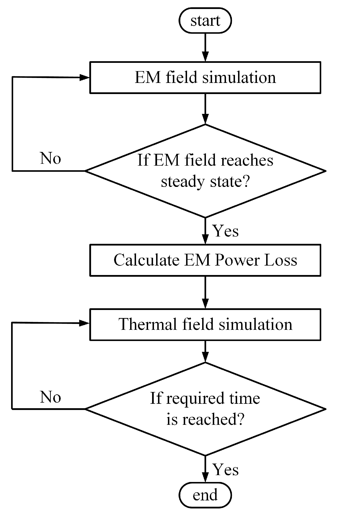
Figure 2.
Spatial distribution of thermal field node and EM field components.

Figure 3.
Structure and dimensions of the planar monopole antenna: (a) side view; (b) top view; (c) bottom view.
Figure 3.
Structure and dimensions of the planar monopole antenna: (a) side view; (b) top view; (c) bottom view.
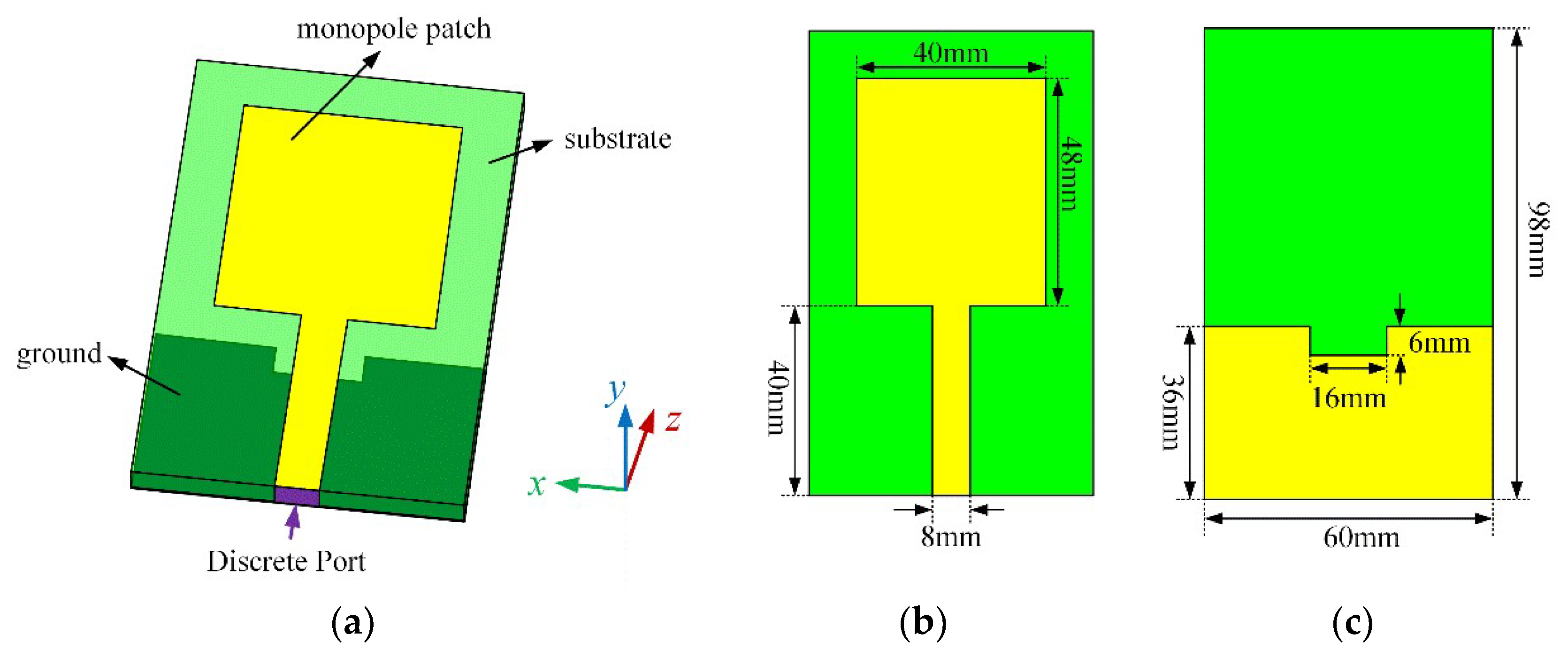
Figure 4.
S11 of the planar monopole antenna.
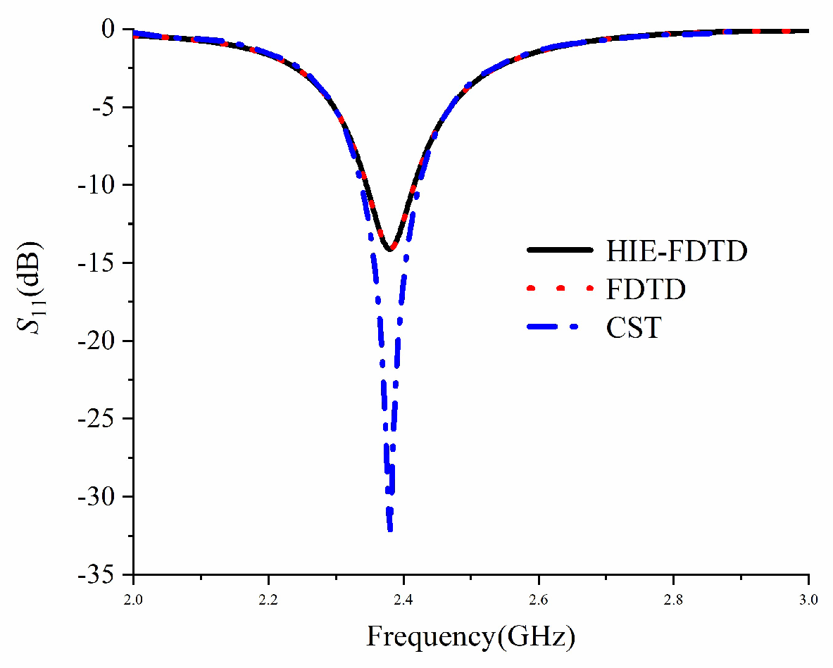
Figure 5.
Directivity patterns of the planar monopole antenna: (a) directivity pattern in xoy plane; (b) directivity pattern in xoz plane.
Figure 5.
Directivity patterns of the planar monopole antenna: (a) directivity pattern in xoy plane; (b) directivity pattern in xoz plane.
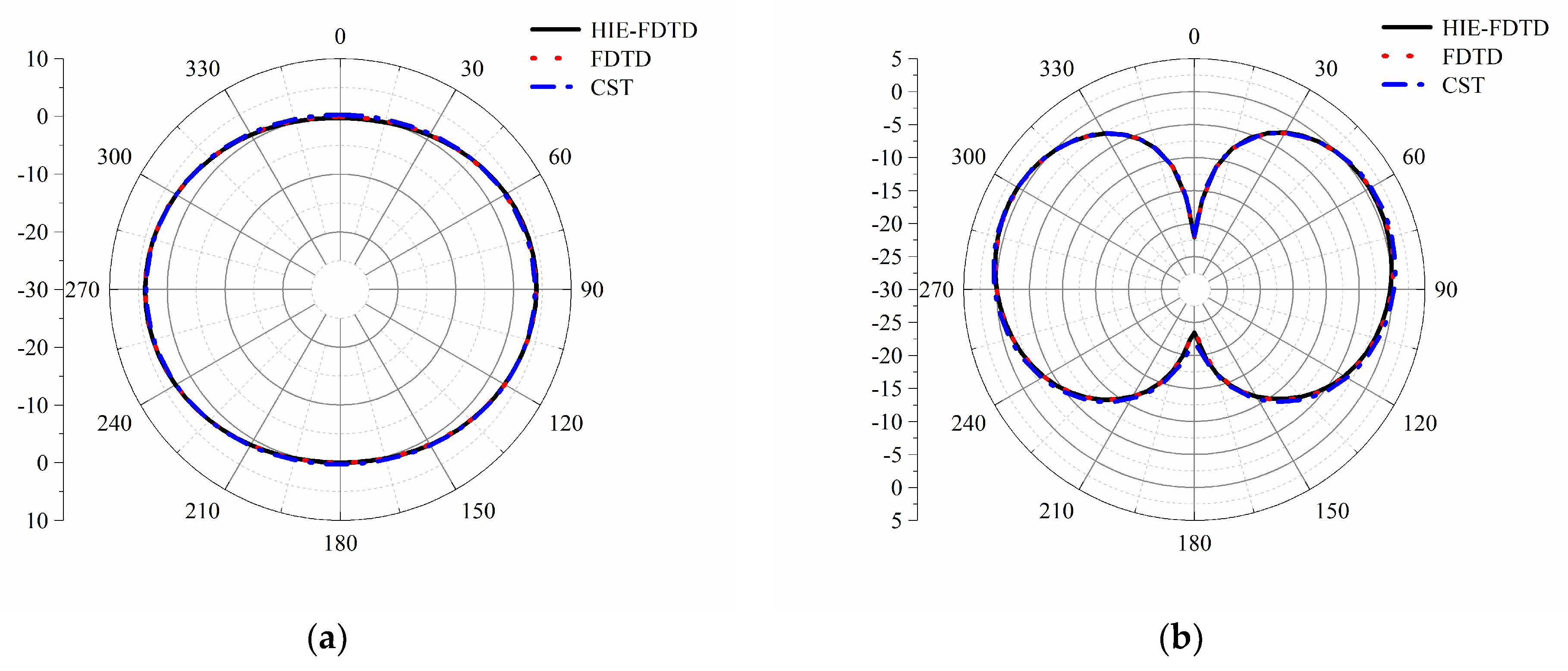
Figure 6.
The thermal field distributions on the surface of the dielectric substrate: (a) by using traditional FDTD-M; (b) by using HIE-FDTD-M.
Figure 6.
The thermal field distributions on the surface of the dielectric substrate: (a) by using traditional FDTD-M; (b) by using HIE-FDTD-M.

Figure 7.
The thermal field distribution on the surface of the dielectric substrate by using COMSOL.
Figure 7.
The thermal field distribution on the surface of the dielectric substrate by using COMSOL.
Publisher’s Note: MDPI stays neutral with regard to jurisdictional claims in published maps and institutional affiliations. |
© 2022 by the authors. Licensee MDPI, Basel, Switzerland. This article is an open access article distributed under the terms and conditions of the Creative Commons Attribution (CC BY) license (https://creativecommons.org/licenses/by/4.0/).
Share and Cite
MDPI and ACS Style
Mou, C.; Chen, J.; Peng, H. Electromagnetic–Thermal Co-Simulation of Planar Monopole Antenna Based on HIE-FDTD Method. Electronics 2022, 11, 4167. https://doi.org/10.3390/electronics11244167
AMA Style
Mou C, Chen J, Peng H. Electromagnetic–Thermal Co-Simulation of Planar Monopole Antenna Based on HIE-FDTD Method. Electronics. 2022; 11(24):4167. https://doi.org/10.3390/electronics11244167
Chicago/Turabian StyleMou, Chunhui, Juan Chen, and Huaiyun Peng. 2022. "Electromagnetic–Thermal Co-Simulation of Planar Monopole Antenna Based on HIE-FDTD Method" Electronics 11, no. 24: 4167. https://doi.org/10.3390/electronics11244167
Note that from the first issue of 2016, this journal uses article numbers instead of page numbers. See further details here.