Global Scattering Center Representation of Target Wide-Angle Single Reflection/Diffraction Mechanisms Based on the Multiple Manifold Concept

Abstract

Many radar applications, such as system design and testing and target detection and recognition, need to compress and rapidly reconstruct the target-scattering characteristics data through some suitable sparse representations, while the scattering center (SC) model resulting from different scattering mechanisms is just a prospective candidate. For the target scattering characteristics data with single reflection/diffraction mechanisms, the multimanifold structures of wide-angle SCs were revealed in light of asymptotic high-frequency theory and ray theory of electromagnetic field. Then the multimanifold clustering and curve/surface fitting algorithms are introduced to construct the target global SC (GSC) model. Compared with simulation data of sphere-cone target, the RCS at elevation ${90}^{°}$, azimuth $0–{180}^{°}$ can be accurately reconstructed by only 77 parameters, the compress rate and root mean square error are 0.66 and 1.17 dB respectively. Simulation results showed that the GSC model could greatly compress the wide-angle scattering data while ensuring a suitable reconstruction accuracy. The proposed multimanifold GSC representation is convenient to implement and can effectively replace the redundant original scattering characteristics data.

1. Introduction

In radar technology, the target scattering characteristics are commonly described by many physical quantities, such as the radar cross section (RCS), high-resolution range profile (HRRP), synthetic aperture radar (SAR) image, etc. These quantities reflect the intrinsic attributes of a target, which are very important in many radar applications, ranging from radar system design to system testing and from target detection to target recognition.

It is necessary to build a database to store the target scattering characteristics data. However, the scattering data are significantly sensitive to the radar’s frequency and view, meaning that the frequency and angle-sampling intervals must be dense enough. Therefore, considering a wideband and whole angle case, the amount of scattering data is expected to be enormous. In view of this, we have to develop a scattering characteristics representation to compress and replace the redundant scattering data.

According to the geometrical theory of diffraction (GTD) [1], the total scattering from an electrically large target can be well-approximated as the superposition of responses from a series of individual scattering centers (SCs). The SC model is a prospective candidate as a sparse representation of target scattering characteristics. Numerous types of SC representation models, such as the ideal point model [2], Prony model [3], GTD model [4], and attributed SC (ASC) model [5], have been proposed, all of which give an expression of frequency and angle.

Some researchers use SC models to compress the scattering characteristics data and rapidly reconstructing them. Zheng et al. [6] proposed a performance-enhanced 2D ESPRIT algorithm to estimate the 2D GTD model parameters and achieve RCS reconstruction. Furthermore, a modified 3D ESPRIT algorithm was developed to carry out parameter estimation of the 3D GTD model and RCS extrapolation [7]. Li et al. [8] introduced a Hankel matrix into the TLS-ESPRIT algorithm to extract GTD SCs and improve the precision of RCS reconstruction. Ghasemi et al. [9] proposed a multistage CLEAN-based method for GTD SCs enumeration and parameter estimation, and achieved HRRP reconstruction. Jing et al. [10] carried out ASC extraction and SAR reconstruction with a genetic algorithm. However, in the above studies, the SCs were extracted using inverse parameter-estimation methods, which require numerous scattering data over a high number of sampling frequencies and angles, resulting in low calculation efficiency. Bhalla et al. [11] proposed an SBR-based method to extract 3D ideal-point SCs at a single frequency and angle. The SBR-based method can avoid scattering data calculation under wideband and wide-angle conditions, which can significantly improve the SC modeling efficiency. Furthermore, Yan et al. [12] derived a formula to calculate the frequency-dependent factors of SC, and then extended Bhalla’s method to the wideband version, which combined the SBR technique with the GTD model [13]. Therefore, Yan’s method had a stronger frequency-domain extrapolation ability and higher data compression performance.

However, the aforementioned SC models are unable to represent the complex angular dependence of target scattering, resulting in a weak extrapolation ability in the angular domain. To address this problem, many researchers have attempted to construct a global SC (GSC) representation model that is valid over the whole angular domain. The main idea behind constructing the GSC model was to establish a correspondence between SCs at various aspect angles. Bhalla et al. [14] transformed the SCs’ positions to a global target-centered coordinate system and used a voxel-based method to construct the GSC model. Zhou et al. [15,16] used the Hough transform to associate the SCs at different angles. Hu et al. [17] constructed the GSC model from HRRPs using the RANSAC algorithm. It is worth noting that these methods are only applicable for fixed SCs that are stationary across aspect angles. However, for the real target, there are also unfixed SCs that are distributed or sliding with the change of radar view [18]. Considering this phenomenon, the authors of [19,20] developed a new method to construct the GSC model using the nearest-neighbor clustering algorithm, which is suitable for fixed, distributed and sliding SCs. However, the selection of initial values and noise points may seriously affect the clustering effect. Furthermore, an OPTICS-based method was developed in [21], although it has difficulties separating different SC clusters that are adjacent or intersected. In summary, the existing methods of GSCs modeling have poor performance for cases where fixed, distributed and sliding GSCs exist simultaneously, or the case where the GSCs are adjacent or intersected with each other.

In this paper, for the target scattering characteristics data with single reflection/diffraction mechanism, we develop a GSC representation based on the multiple manifold concept, and further introduce a multimanifold clustering and curve/surface fitting algorithm to construct the target GSC model. The proposed approach was able to improve the extrapolation ability and compression performance of the angular domain. The remainder of this paper is organized as follows. In Section 2, the multimanifold structures of wide-angle SCs are revealed in light of asymptotic high-frequency theory and ray theory of the electromagnetic (EM) field. In Section 3, the multimanifold clustering algorithm is applied to associate the wide-angle 3D SCs, and the whole data processing flow is described. In Section 4, simulation experiments are implemented to validate the proposed method. Section 5 concludes this paper.

2. Principle

In essence, the SC phenomenon is generally caused by the spatial localization effect of high-frequency scattering. Usually, the general form of a SC model is

$$S(k,\widehat{r})={\displaystyle \sum _{m=1}^M{A}_m(k,\widehat{r})e^{\mathrm{j}2k\widehat{r}·x_m(\widehat{r})}}$$

(1)

where $k=2\pi f/c$ is the wave number, $f$ is the frequency, $c$ is the velocity of propagation, $\widehat{r}$ is the unit vector of radar view, $S$ is the scalar complex RCS in a specific transmitting and receiving polarization, and $A_m$ and ${\mathit{x}}_m$ are the amplitude and location of the m-th SC, respectively.

In traditional SC concepts, the SC amplitude and location are constant and, thus, are only suitable for a narrow range of frequencies and angles, which is not economical when dealing with wide-angle scattering data. From the view of GSC, SCs at various angles are interrelated, and, thus, the amplitude and location of each SC are functions of the frequency and angle in the whole parameter domain.

From theories based on asymptotic high-frequency theory and ray theory, such as geometrical optics (GO), GTD, physical optics (PO) and the physical theory of diffraction (PTD), an SC representation with a frequency and radar view can be derived [22]. In this paper, we mainly focus on the relationship between SC locations, ${\mathit{x}}_m$, and the radar view, $\widehat{r}$.

2.1. Relationship between SC Locations and Radar View Based on GO/GTD

It is supposed that a linearly polarized plane wave illuminates on a patch-wise smooth, electrically large and perfect electric conducting (PEC) target. Based on the GO theory [23], the incident plane wave is seen as a beam of parallel rays shooting toward the target zone and bouncing once or more times on the target surface. In this paper, we only consider the single- and backward-scattering situation.

The single-scattering mechanisms of a nonstealth target mainly include specular reflection, edge diffraction and tip/corner diffraction.

For the specular reflection mechanism, the formation of an SC from a doubly curved surface can be depicted as in Figure 1.

Obviously, for a smooth patch of the curved surface, there is only one ray (red line in Figure 1) that can return to the radar. Then, this ray’s bouncing point on the surface patch can be seen as an effective SC (red point in Figure 1).

Let ${\mathit{x}}^{\mathrm{sc}}$ be the location of the bouncing point or SC and ${\widehat{r}}_{\mathrm{sc}}$ be the visible view vector of GSC; then, based on GO, ${\mathit{x}}^{\mathrm{sc}}$ and ${\widehat{r}}_{\mathrm{sc}}$ satisfy the constraints as follows:

$${\widehat{r}}_{\mathrm{sc}}·{\mathit{x}}_u^{\mathrm{sc}}={\widehat{r}}_{\mathrm{sc}}·{\mathit{x}}_v^{\mathrm{sc}}=0$$

(2)

where $(u,v)$ are the coordinates of two principal directions of the surface patch and ${\mathit{x}}_u^{\mathrm{sc}}$ and ${\mathit{x}}_v^{\mathrm{sc}}$ are the partial derivatives of $\mathit{x}(u,v)$ at ${\mathit{x}}^{\mathrm{sc}}$, and ${\mathit{x}}^{\mathrm{sc}}$, respectively, which naturally satisfies

$${\mathit{x}}^{\mathrm{sc}}=\mathit{x}(u_{\mathrm{sc}},v_{\mathrm{sc}}), (u_{\mathrm{sc}},v_{\mathrm{sc}})\in D^2$$

(3)

where $D^2$ is the 2D visible domain of $(u,v)$ illuminated by an incident ray.

${\mathit{x}}^{\mathrm{sc}}$ will change as ${\widehat{r}}_{\mathrm{sc}}$ changes from (2). We use $P^{\alpha }$ and $C^{\gamma }$ to represent the subspaces of ${\mathit{x}}^{\mathrm{sc}}$ in a single view and all views, respectively, and use $N^{\beta }$ and ${\mathsf{\Omega }}^{\delta }$ to represent the subspace of ${\widehat{r}}_{\mathrm{sc}}$ in a fixed location and all possible locations, respectively, where $\alpha ,\beta ,\gamma ,\delta$ are the extended dimensions.

We can rewrite (3) as a set:

$$X_m=\left\{{\mathit{x}}^{\mathrm{sc}}\right|{\mathit{x}}^{\mathrm{sc}}=\mathit{x}(u_{\mathrm{sc}},v_{\mathrm{sc}})\}\to P^0\subset C^2\subset R^3$$

(4)

where $m$ is the SC index, $P^0$ is a 0D subspace (i.e., point) of the 3D vector space, $R^3$, in a fixed view, which indicates that the SC is localized.

However, when various views are considered, all $P^0$ form a 2D continuous subspace in $R^3$, which is usually seen as a sliding SC. Then, from the constraint relation of ${\mathit{x}}^{\mathrm{sc}}$ and ${\widehat{r}}_{\mathrm{sc}}$ in (2), we can conclude the set representation of ${\widehat{r}}_{\mathrm{sc}}$ as follows:

$$R_m=\left\{{\widehat{r}}_{\mathrm{sc}}\right|{\widehat{r}}_{\mathrm{sc}}=\widehat{n}(u_{\mathrm{sc}},v_{\mathrm{sc}})\}\to N^0\subset {\mathsf{\Omega }}^2\subset S^2$$

(5)

where $\widehat{n}(u_{sc},v_{sc})$ is the normal vector at the SC location.

As each ${\mathit{x}}^{\mathrm{sc}}$ corresponds to a single ${\widehat{r}}_{\mathrm{sc}}$, $R_m$ is a point set with unit length (denoted as $N^0$). However, when various possible locations are considered, all $R_m$ form a 2D subspace (i.e., solid angle range), ${\mathsf{\Omega }}^2$, of the unit sphere, $S^2$.

For the edge diffraction mechanism, the formation of a SC from a nonaxially incident curved edge is depicted in Figure 2.

Based on GTD theory [1], edge-diffracted rays are distributed on a conical surface, called a Keller cone (as in Figure 2). Similar to the case of specular reflection, there is still only one ray that can return the radar, and the ray’s diffracted point on the edge can be seen as an effective SC.

Then, ${\mathit{x}}^{\mathrm{sc}}$ and ${\widehat{r}}_{\mathrm{sc}}$ satisfy the constraints as follows:

$${\widehat{r}}_{\mathrm{sc}}·{\mathit{x}}_t^{\mathrm{sc}}=0$$

(6)

where $t$ is the coordinate of edge segment parameter, ${\mathit{x}}_t^{\mathrm{sc}}$ is the derivative of $\mathit{x}(t)$ at ${\mathit{x}}^{\mathrm{sc}}$ and ${\mathit{x}}^{\mathrm{sc}}$ naturally satisfies

$${\mathit{x}}^{\mathrm{sc}}=\mathit{x}(t_{\mathrm{sc}}), t_{\mathrm{sc}}\in D^1=[t_1,t_2]$$

(7)

where $D^1$ corresponds to the edge segment illuminated by an incident ray.

Similar to the previous example, we can also rewrite (7) as a set:

$$X_m=\left\{{\mathit{x}}^{\mathrm{sc}}\right|{\mathit{x}}^{\mathrm{sc}}=\mathit{x}(t_{\mathrm{sc}})\}\to P^0\subset C^1\subset R^3$$

(8)

where $P^0$ is still a 0D subspace of $R^3$ in a fixed view.

However, when various views are considered, all $P^0$ form a 1D continuous subspace in $R^3$, which is also seen as a sliding SC. Then, from the constraint relation of ${\mathit{x}}^{\mathrm{sc}}$ and ${\widehat{r}}_{\mathrm{sc}}$ in (6), we can conclude the set representation of ${\widehat{r}}_{\mathrm{sc}}$ as follows:

$$R_m=\left\{{\widehat{r}}_{\mathrm{sc}}\right|{\widehat{r}}_{\mathrm{sc}}·{\mathit{x}}_t^{\mathrm{sc}}=0\}\to N^1\subset {\mathsf{\Omega }}^2\subset S^2$$

(9)

As each ${\mathit{x}}^{\mathrm{sc}}$ corresponds to an infinite number of ${\widehat{r}}_{\mathrm{sc}}$, $R_m$ is a 1D vector subspace with a unit length (denoted as $N^1$). However, when various locations are considered, all $R_m$ form a 2D subspace, ${\mathsf{\Omega }}^2$, of $S^2$.

For the tip/corner diffraction mechanism, the formation of an SC is depicted in Figure 3. Based on the GTD theory, still only one ray can return the radar and the diffraction point is just the tip/corner point.

$${\mathit{x}}^{\mathrm{sc}}={\mathit{x}}_{\mathrm{tip}/\mathrm{corner}}$$

(10)

Moreover, we can rewrite (10) as a set:

$$X_m=\left\{{\mathit{x}}^{\mathrm{sc}}\right|{\mathit{x}}^{\mathrm{sc}}={\mathit{x}}_{\mathrm{tip}/\mathrm{corner}}\}\to P^0=C^0\subset R^3$$

(11)

where all $P^0$ form a 0D subspace of $R^3$ in multiple views, which is usually called a fixed SC. The set representation of ${\widehat{r}}_{\mathrm{sc}}$ is

$$R_m=\left\{{\widehat{r}}_{\mathrm{sc}}\right|\mathrm{All} \mathrm{directions} \mathrm{except} \mathrm{angles} \mathrm{occupied} \mathrm{by} \mathrm{target}\}\to N^2={\mathsf{\Omega }}^2\subset S^2$$

(12)

As each ${\mathit{x}}^{\mathrm{sc}}$ corresponds to an infinite number of ${\widehat{r}}_{\mathrm{sc}}$, all $R_m$ form a 2D subspace, ${\mathsf{\Omega }}^2$, of $S^2$.

Based on the above discussions, all GSCs from the doubly curved surface, curved edge and tip/corner structures are point or localized SCs. However, according to the ASC model, a distributed SC also exists, which can present as straight segments [5]. Unfortunately, the curvatures of the target’s surface or edge would be zero in this case, which makes GO and GTD singular. In Section 2.2, this problem will be solved using PO and PTD.

2.2. Relationship between SC Locations and Radar View Based on PO/PTD

Under monostation and far field conditions, the PO formula [24] for calculating target scattering can be simply expressed by a double integral:

$$S(k)=-\frac{\mathrm{j}k}{\sqrt{\pi }}{\displaystyle \iint f^{\prime }(u,v)e^{\mathrm{j}kg(u,v)}\mathrm{d}u\mathrm{d}v}$$

(13)

Using the stationary phase method (SPM) [24], under nondegenerate conditions, the double integral (13) approximates the total contributions at three kinds of critical points, which correspond to three types of SCs discussed earlier from GO/GTD theory. Thus, we mainly focus on the degenerate condition, i.e., $g_{uu}(u,v)·g_{vv}(u,v)=0$, where GO/GTD fails.

The degenerate condition indicates that at least one of the terms $g_{uu}$ and $g_{vv}$ equals 0, as discussed in two cases.

Case 1: $g_{uu}\ne 0$, $g_{vv}=0$. We have $\widehat{r}·{\mathit{x}}_{vv}(u,v)=0$.

According to SPM, there is $g_u(u_s,v)=g_v(u_s,v)=0$. Then, when no high-order SPP exists, we have

$${\widehat{r}}_{\mathrm{sc}}·{\mathit{x}}_u(u_s,v)={\widehat{r}}_{\mathrm{sc}}·{\mathit{x}}_v(u_s,v)=0,\hspace{1em}v\in [v_1,v_2]$$

(14)

It is not hard to obtain $\widehat{n}(u,v)·{\mathit{x}}_{vv}(u,v)=0$, resulting in ${\mathit{x}}_{vv}=0$ or $\widehat{n}\perp {\mathit{x}}_{vv}$, which corresponds to a singly curved surface and torus surface, respectively. Unlike the previous cases, there are countless rays that can return the radar, as illustrated in Figure 4. Therefore, the SP ‘point’ is no more a single point but a line or curve segment belonging to the distributed SC.

The SC position and visible view of the singly curved surface can then be written as a set:

$$X_m=\left\{{\mathit{x}}^{\mathrm{sc}}\right|{\mathit{x}}^{\mathrm{sc}}=\mathit{x}(u_s,v), v\in [v_1,v_2]\}\to P^1\subset C^2\subset R^3$$

(15)

$$R_m=\left\{{\widehat{r}}_{\mathrm{sc}}\right|{\widehat{r}}_{\mathrm{sc}}=\widehat{n}(u_s,v), \mathrm{any} v\in [v_1,v_2]\}\to N^0\subset {\mathsf{\Omega }}^1\subset S^2$$

(16)

The SC position and visible view of the torus surface can be written as a set:

$$X_m=\left\{{\mathit{x}}^{\mathrm{sc}}\right|{\mathit{x}}^{\mathrm{sc}}=\mathit{x}(u_s,v), v\in [v_1,v_2]\}\to P^2=C^2\subset R^3$$

(17)

$$R_m=\left\{{\widehat{r}}_{\mathrm{sc}}\right|{\widehat{r}}_{\mathrm{sc}}=\widehat{n}(u_s,v), \mathrm{any} v\in [v_1,v_2]\}\to N^0={\mathsf{\Omega }}^0\subset S^2$$

(18)

Case 2: $g_{uu}=g_{vv}=0$.

According to SPM, there is $x_{uu}(u,v)=x_{vv}(u,v)=0$. When no high-order SPP exists, we have

$$\widehat{r}·{\mathit{x}}_u(u,v)=\widehat{r}·{\mathit{x}}_v(u,v)=0, (u,v)\in D$$

(19)

Furthermore, there are countless rays that can return the radar, as depicted in Figure 5. All points on the plane are seen as SCs, which belong to the planar-distributed SC.

The SC position and visible view can then be written as a set:

$$X_m=\left\{{\mathit{x}}^{\mathrm{sc}}\right|{\mathit{x}}^{\mathrm{sc}}=\mathit{x}(u,v), (u,v)\in D\}\to P^2=C^2\subset R^3$$

(20)

$$R_m=\left\{{\widehat{r}}_{\mathrm{sc}}|{\widehat{r}}_{\mathrm{sc}}=\widehat{n}(u,v), \mathrm{any} (u,v)\in D\right\}\to N^0={\mathsf{\Omega }}^0\subset S^2$$

(21)

It should be noted that the SCs’ characteristics under PO degenerate conditions on the interior of the surface patch have been discussed previously. However, when the degenerate condition is satisfied on the boundary, the edge diffraction must be considered. According to PTD theory [25], the contribution of edge diffraction can be represented as a 1D integral.

From the SPM, the SC position and visible aspect satisfy the relation as follows:

$$g_t={\widehat{r}}_{\mathrm{sc}}·{\mathit{x}}_t^{\mathrm{sc}}=0$$

(22)

Under the degenerate condition, we have

$$g_{tt}={\widehat{r}}_{\mathrm{sc}}·{\mathit{x}}_{tt}^{\mathrm{sc}}=0$$

(23)

It is not hard to obtain ${\mathit{x}}_{tt}^{\mathrm{sc}}=0$ or ${\widehat{r}}_{\mathrm{sc}}\perp {\mathit{x}}_{tt}^{\mathrm{sc}}$, which corresponds to a straight edge or an axially incident circular edge, as depicted in Figure 6.

The SC position and visible view of the straight edge can be written as a set:

$$X_m=\left\{{\mathit{x}}^{\mathrm{sc}}\right|{\mathit{x}}^{\mathrm{sc}}=\mathit{x}(t_{\mathrm{sc}}), t_{\mathrm{sc}}\in [t_1,t_2]\}\to P^1=C^1\subset R^3$$

(24)

$$R_m=\left\{{\widehat{r}}_{\mathrm{sc}}\right|{\widehat{r}}_{\mathrm{sc}}=\widehat{a}\times \widehat{t}, \widehat{a} \mathrm{is} \mathrm{any} \mathrm{unit} \mathrm{vector}\}\to N^1={\mathsf{\Omega }}^1\subset S^2$$

(25)

where $\widehat{t}$ is the direction of the straight edge.

The SC position and visible view of the circular edge can be written as a set:

$$X_m=\left\{{\mathit{x}}^{\mathrm{sc}}\right|{\mathit{x}}^{\mathrm{sc}}=\mathit{x}(t_{\mathrm{sc}}), t_{\mathrm{sc}}\in [t_1,t_2]\}\to P^2=C^2\subset R^3$$

(26)

$$R_m=\left\{{\widehat{r}}_{\mathrm{sc}}\right|{\widehat{r}}_{\mathrm{sc}}={\widehat{b}}_e\}\to N^0={\mathsf{\Omega }}^0\subset S^2$$

(27)

where ${\widehat{b}}_e$ is the binormal of the circular edge.

2.3. 6D Feature Space Combining SC Locations with Radar View and Its Multimanifold Data Structure

Now, let us summarize the eight scattering structures discussed above, which can be classified into six GSC types. The scattering structures, GSC types and subspace dimensions are shown in

Table 1. The GSC types and subspace dimensions of eight scattering structures.

Scattering Structures	GSC Types *	$\mathit{\alpha }$	$\mathit{\beta }$	$\mathit{\gamma }$	$\mathit{\delta }$
Doubly curved surface	SS	0	0	2	2
Singly curved surface	SD	1	0	2	1
Torus surface	DD	2	0	2	0
Plate	DD	2	0	2	0
Curved edge (nonaxially incident)	FS	0	1	1	2
Circular edge (axially incident)	DD	2	0	2	0
Straight edge	FD	1	1	1	1
Tip/corner	FF	0	2	0	2

* F, S, D represent the fixed, sliding and distributed SC, respectively.

. The GSC types can be determined with the 2D description of SCs [26]. The meaning of $\alpha ,\beta ,\gamma ,\delta$ was explained in Section 2.1.

There are several deductions from Table 1, as follows:

(1) Different scattering structures correspond to different GSC types, and have different dimension characteristics for $P/N/C/\mathsf{\Omega }$;

(2) From the constraints of ${\widehat{r}}_{\mathrm{sc}}$ and ${\mathit{x}}^{\mathrm{sc}}$ for all GSC types, we can deduce that all ${\widehat{r}}_{\mathrm{sc}}$ support space, $N^{\beta }$, and this is the normal space of ${\mathit{x}}^{\mathrm{sc}}$’s support space, $P^{\alpha }$;

(3) There exists a relation for any GSC type:

$$\alpha +\delta \equiv \beta +\gamma \equiv 2$$

(28)

which indicates that the combined subspace of the SC location vector, ${\mathit{x}}^{\mathrm{sc}}$, and view vector, ${\widehat{r}}_{\mathrm{sc}}$, has a fixed dimension.

We defined a combined 6D feature vector $({\mathit{x}}^{\mathrm{sc}},{\widehat{r}}_{\mathrm{sc}})$, so the 6D features corresponding to the GSCs in Table 1 must fall into a 2D subspace, although different types of GSCs map to different subspaces.

As the surface or edge is smooth either patch-wise or segment-wise, we can conclude that the 2D subspace of 6D feature vectors will be a 2D manifold in the 6D feature space. Therefore, the GSC data integrity represented as 6D feature vectors has a multimanifold structure, i.e., the combination of a series of 2D submanifolds, each of which corresponds to a GSC from a specific scattering structure.

A manifold is a very important mathematical concept and tool used to represent and analyze a complex data set. In the remainder of this paper, based on the above conclusions on the multimanifold structure of the GSC data, we will utilize the multimanifold clustering algorithm to associate SCs at various angles and realize the GSC representation of wide-angle scattering data.

3. Algorithm

3.1. Multimanifold Clustering

Wide-angle SCs can be associated using the clustering algorithm. However, the submanifolds of wide-angle SCs may be adjacent or even intersecting, which would greatly increase the difficulty of clustering. The spectral multimanifold clustering (SMMC) [27] algorithm can disassemble intersected points to obtain the components of different submanifolds, solving the above problem. In the SMMC algorithm, the tangent space-related structural similarity and the Euclidean distance-related local similarity are combined to construct a more appropriate similarity matrix, and then the multimanifold clustering results can be obtained using the classical spectral method. Firstly, multiple local linear manifolds are trained using MPPCA [28] to approximate SCs’ submanifolds, and then the tangent space of each SC point is estimated according to the principal subspace of the corresponding analyzer. Suppose that the tangent space at point $x_a$ is ${\mathsf{\Theta }}_a$, then the structural similarity between the tangent spaces of $x_a$ and $x_b$ is defined as

$$p_{ab}=p({\mathsf{\Theta }}_a,{\mathsf{\Theta }}_b)={\left({\displaystyle \prod _{l=1}^d\cos {\theta }_l}\right)}^o$$

(29)

where $d$ is the dimension of submanifold, ${\theta }_l$ is the principal angle between two tangent spaces and $o$ is an adjustable parameter.

The local similarity, which measures the Euclidean distance relationship between $x_a$ and $x_b$, is defined as

$$q_{ab}=\{\begin{array}{cc}1& x_a\in \mathrm{Knn}(x_b) \mathrm{or} x_b\in \mathrm{Knn}(x_a)\\ 0& \mathrm{otherwise}\end{array}$$

(30)

where $\mathrm{Knn}(x_a)$ denotes the K nearest-neighbors of $x_a$.

By combining the structural similarity and local similarity, a more appropriate similarity matrix $\mathit{W}$ can be constructed, and the corresponding similarity weight can be expressed as

$$w_{ab}=p_{ab}{q}_{ab}=\{\begin{array}{cc}{\left({\displaystyle \prod _{l=1}^d\cos {\theta }_l}\right)}^o& x_a\in \mathrm{Knn}(x_b) \mathrm{or} x_b\in \mathrm{Knn}(x_a)\\ 0& \mathrm{otherwise}\end{array}$$

(31)

After computing the similarity matrix, the diagonal matrix $\mathit{E}$ can be calculated and the first k-generalized eigenvectors can be extracted with

$$(\mathit{E}-\mathit{W})u=\lambda \mathit{E}u$$

(32)

Finally, the k-means [29] algorithm is applied to cluster the row vectors of $\mathit{U}$ and the clustering results can be obtained. 3D wide-angle SCs belonging to the same typical structure can be effectively associated.

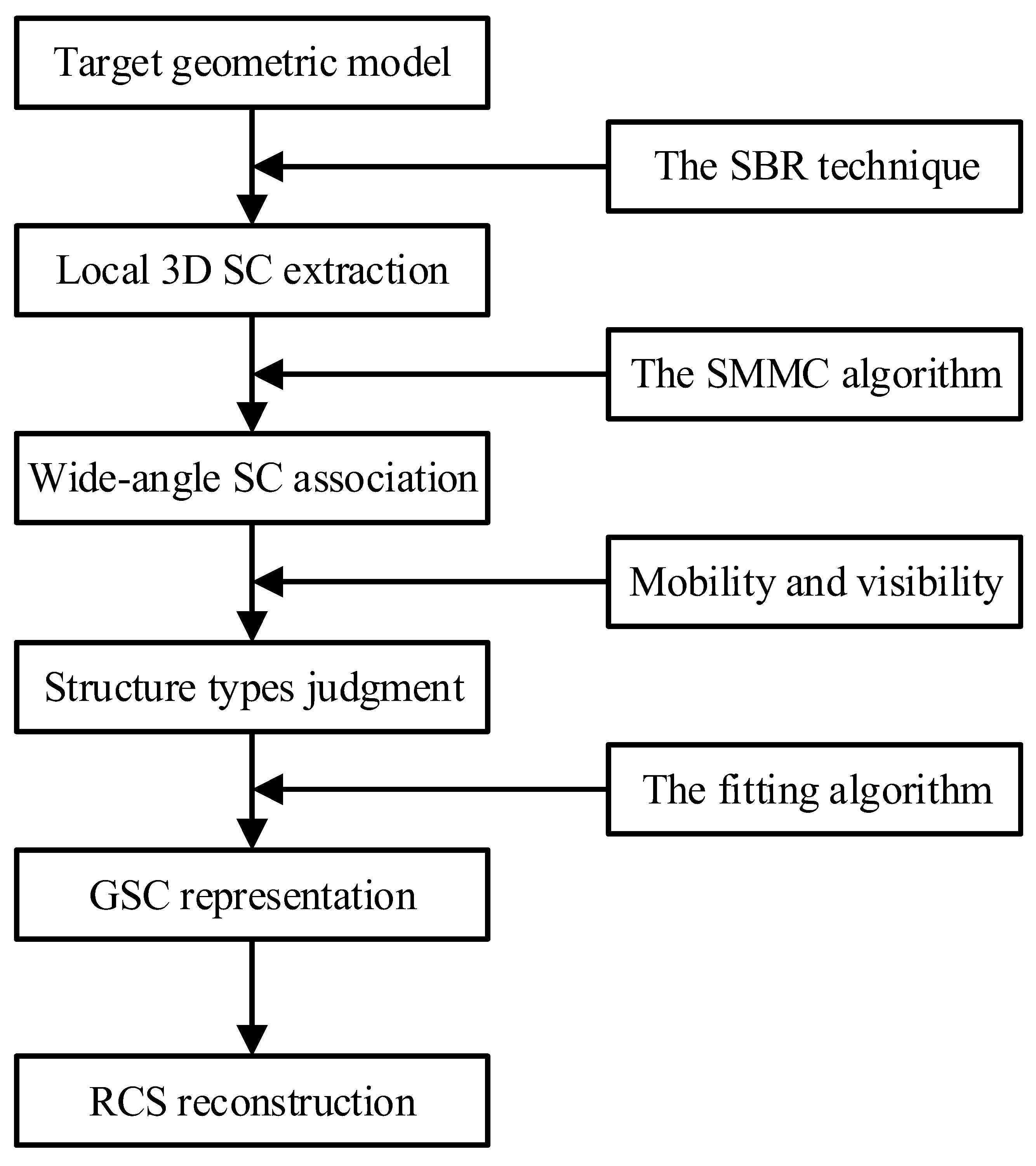
3.2. Data Processing Flow

The data processing flow of the GSC representation is depicted in Figure 7, and it mainly included local 3D SC extraction, wide-angle association of 3D SCs, type judgment of scattering structures and GSC representation. After constructing the GSC model, wide-angle RCS could be reconstructed directly.

3.2.1. Local 3D SC Extraction

Given the target geometric model and radar parameters, the ray paths and fields data were calculated using the SBR [30] technique. The ray-tube integration method was then applied to quickly generate the 3D ISAR image of the target; the ray-tube integration formula [31] is

$$I(x,y,z)=[{\displaystyle \sum _{i \mathrm{rays}}{\alpha }_i}\delta (x-{x^{\prime }}_i,\mathrm{y}-{y^{\prime }}_i,z-{z^{\prime }}_i)]\ast h(x,y,\mathrm{z})$$

(33)

where $\ast$ denotes the convolution operation; $\delta (·,·,·)$ is the 3D Dirac function; $z$, $x$ and $y$ are the down range and two orthogonal cross range directions, respectively; ${\alpha }_i$ is the scattering field of the i-th ray; ${z^{\prime }}_i$, ${x^{\prime }}_i$ and ${y^{\prime }}_i$ respectively the down range and cross range positions, respectively; and $h(x,y,\mathrm{z})$ is the ray spread function.

After obtaining the 3D ISAR image, the target local 3D SCs could be further extracted using the CLEAN [32] algorithm. Specifically, the amplitude and position parameters of the corresponding SC were extracted by iteratively searching the peak points in the residual ISAR image, and then the point spread response of the SC was eliminated from the ISAR image. When the peak value of the residual ISAR image was lower than a preset threshold, the iterative process was terminated and the local SCs were completely extracted.

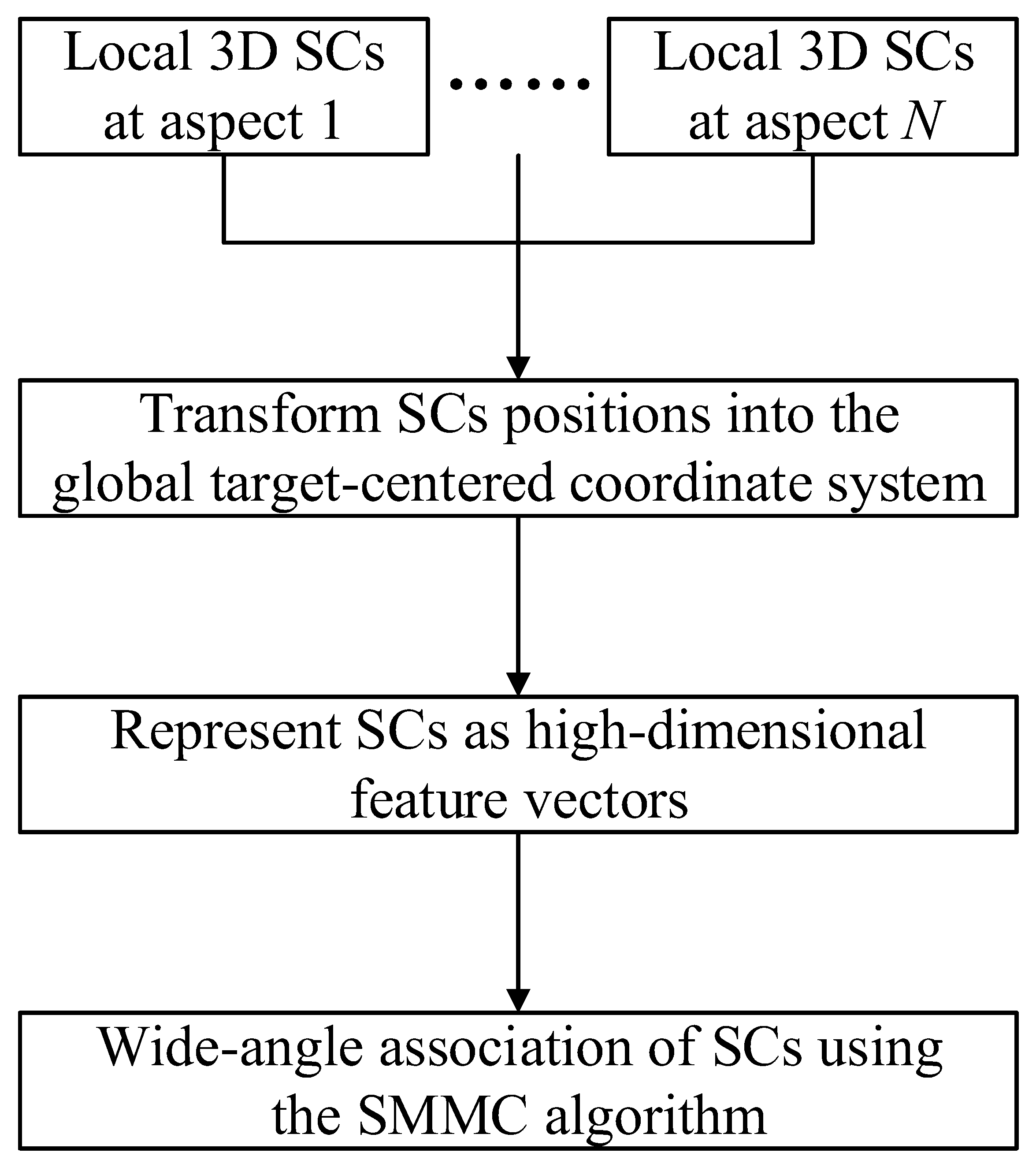
3.2.2. Wide-Angle Association of 3D SCs

To fully characterize a target at all aspects, 3D SC extraction needs to be executed at various angles on a grid in terms of both the elevation and azimuth. After obtaining the local 3D SCs at various aspects, the work flow depicted in Figure 8 of wide-angle association using the SMMC algorithm was followed.

As a first step, the SCs’ positions were transformed from the radar coordinate system into the global target-centered coordinate system.

According to the principle in Section 2, the SCs’ distribution may differ in different feature spaces, and accurate SCs association needs to be carried out in an appropriate feature space. All SCs were first sorted according to their scattering bounce time, after which SC data were further represented as 6D feature vectors $(x,y,z,\sin \theta \cos \varphi ,\sin \theta \sin \varphi ,\cos \theta )$.

Finally, according to the principle in Section 3.1, the SMMC algorithm was adopted to achieve wide-angle association of SCs in the 6D feature space.

3.2.3. Type Judgment of Scattering Structures

After achieving the wide-angle association, the type judgment of scattering structures can be further realized based on the SCs’ mobility and visibility. Considering any structure, the spatial mobility in the $x$, $y$ and $z$ directions of SCs can be evaluated by the amplitude-weighted standard deviation, which can be expressed as

$$\begin{array}{l}{\sigma }_x=\mathrm{std}(x,A)=\sqrt{[{\displaystyle \sum _{i=1}^N{A}_i{(x_i-\overline{x})}^2}]/({\displaystyle \sum _{i=1}^N{A}_i})}\\ {\sigma }_y=\mathrm{std}(y,A)=\sqrt{[{\displaystyle \sum _{i=1}^N{A}_i{(y_i-\overline{y})}^2}]/({\displaystyle \sum _{i=1}^N{A}_i})}\\ {\sigma }_z=\mathrm{std}(z,A)=\sqrt{[{\displaystyle \sum _{i=1}^N{A}_i{(z_i-\overline{z})}^2}]/({\displaystyle \sum _{i=1}^N{A}_i})}\end{array}$$

(34)

where $N$ is the number of SCs corresponding to the structure, $A_i$, and $(x_i,y_i,z_i)$ denote the amplitude and location of each SC. $(\overline{x},\overline{y},\overline{z})$ denote the amplitude-weighted average location.

The angle visibility in the elevation and azimuth direction of SCs can be evaluated by the visibility rate, $V_{\theta }$ and $V_{\varphi }$, which can be expressed as

$$\begin{array}{l}{V}_{\theta }=\frac{{\theta }_{\mathrm{visible}}}{{\theta }_{\mathrm{all}}}\times 100\%\\ V_{\varphi }=\frac{{\varphi }_{\mathrm{visible}}}{{\varphi }_{\mathrm{all}}}\times 100\%\end{array}$$

(35)

where ${\theta }_{\mathrm{all}}$ and ${\varphi }_{\mathrm{all}}$ denote the total number of elevation and azimuth angles for SC extraction, respectively, and ${\theta }_{\mathrm{visible}}$ and ${\varphi }_{\mathrm{visible}}$ denote the number of visible elevation and azimuth angles, respectively.

Obviously, with larger values of ${\sigma }_x$, ${\sigma }_y$ and ${\sigma }_z$, the higher the dispersion degree in the $x$, $y$ and $z$ directions is, and the stronger the spatial mobility of SCs. The larger the values of $V_{\theta }$ and $V_{\varphi }$ are, the stronger the angle visibility in the elevation and azimuth directions.

3.2.4. GSC Representation

The associated GSC amplitude of each scattering structure is smooth and has various angles, which can be represented by a 2D polynomial surface.

Similarly, considering different scattering structure types, appropriate curve/surface fitting algorithms were applied to realize the GSC locations’ representation. The SCs of FF, FD and DD structures are generally fixed/distributed in the elevation and azimuth directions, which can be represented as an amplitude-weighted average location. The SCs of FS and SD structures are generally fixed/distributed in the elevation/azimuth direction and sliding in the other direction, which can be represented as an amplitude-weighted average location and polynomial curve function. The SCs of an SS structure are generally sliding in both the elevation and azimuth direction, which can be represented as a 2D polynomial surface function.

After representing the GSC amplitudes and equivalent locations of all scattering structures, the target GSC model was constructed and the target wide-angle RCS could be reconstructed directly.

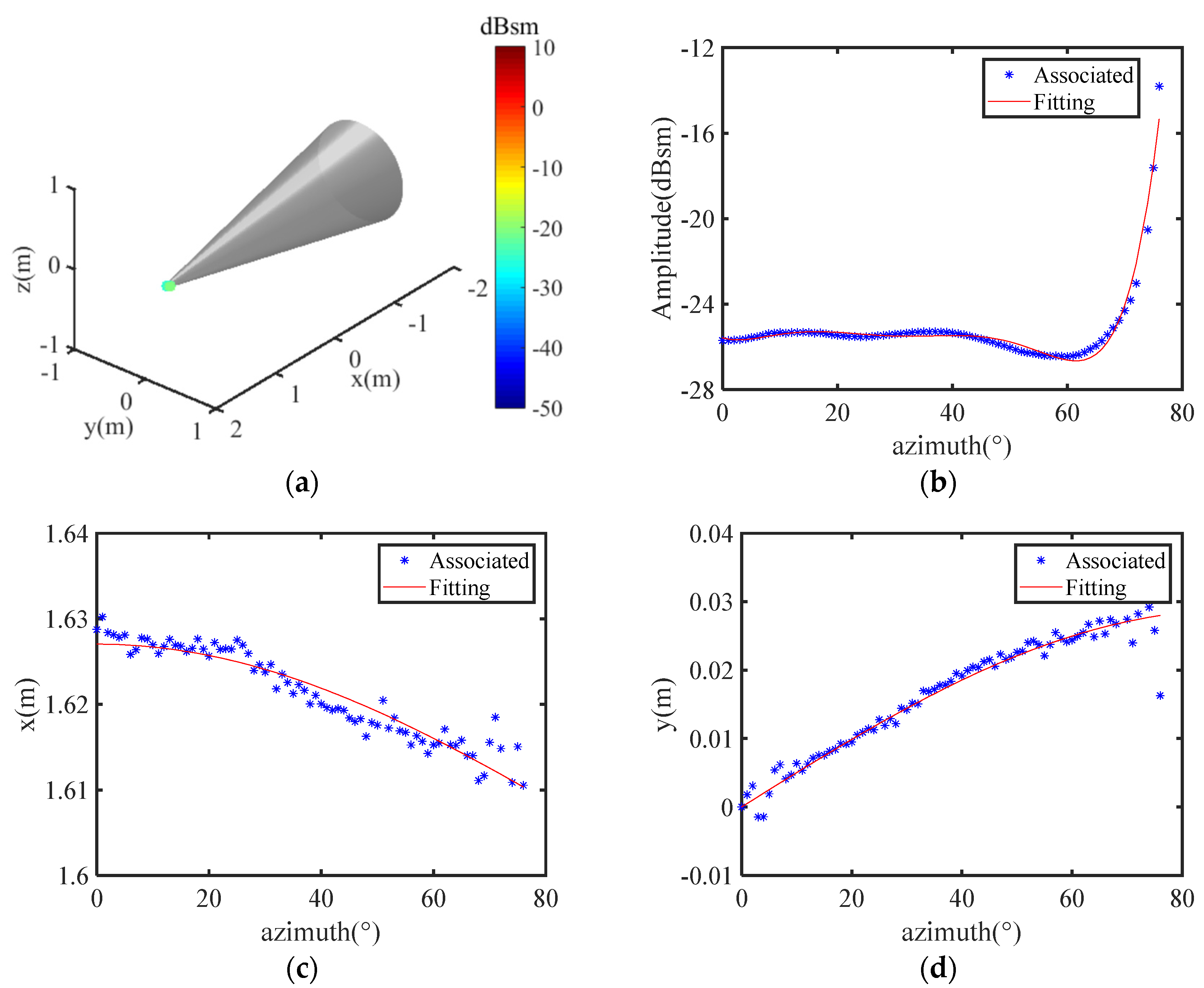
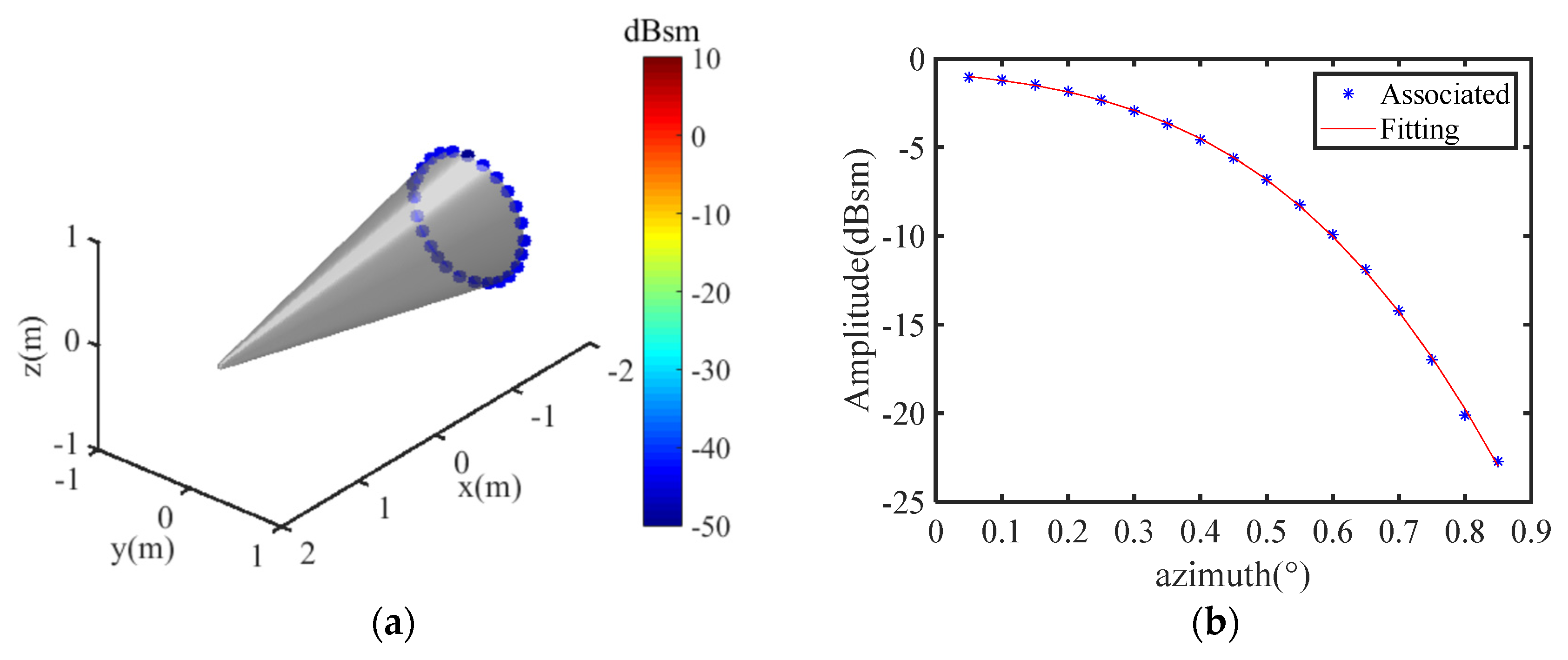
4. Simulation Results

In this paper, the PEC sphere-cone target was taken as an example to validate the effectiveness of the GSC representation. The size of the sphere-cone was $2.7 \mathrm{m} \times 1 \mathrm{m} \times 1 \mathrm{m}$. Due to the axial symmetry, only a single elevation angle was considered. The six GSC types in Table 1 were naturally degraded into fixed, sliding and distributed types. Furthermore, the 6D feature vector was degraded to a 5D feature vector $(x,y,z,\cos \varphi ,\sin \varphi )$. The conditions of 3D SC extraction were as follows: elevation angle ${90}^{°}$, azimuth angle $0–{180}^{°}$, V-V polarization, center frequency 10 GHz, bandwidth 1 GHz. After obtaining the local 3D SCs at various aspects, the SMMC algorithm was used to achieve wide-angle association in a 5D feature space. The result of wide-angle association is shown in Figure 9, which indicated that 3D wide-angle SCs belonging to the spherical head, conical surface, circular edge, bottom surface, right-curved edge and left-curved edge were correctly associated and separated.

The scattering types of six canonical structures on the sphere-cone are shown in

Table 2. The scattering types of six canonical structures on the sphere-cone target.

Canonical Structure	${\mathit{\sigma }}_{\mathit{x}}$	${\mathit{\sigma }}_{\mathit{y}}$	${\mathit{V}}_{\mathit{\varphi }}/\%$	Scattering Type
spherical head	0.07	0.09	44.20	Sliding
conical surface	0.95	0.40	0.33	Distributed
circular edge	0	0.65	0.55	Distributed
bottom surface	0	0.54	0.47	Distributed
right-curved edge	0.0018	0.0019	91.71	Fixed
left-curved edge	0.0033	0.0032	33.70	Fixed

and the location standard deviation and angle visibility rate are also shown.

The SCs of the spherical head structure had little mobility in the $x$ and $y$ directions and a strong visibility in the azimuth direction. Therefore, the spherical head had a sliding scattering structure. The SCs of the conical surface structure had strong mobility in the $x$ and $y$ directions, and were hardly visible in the azimuth direction. The SCs of the circular edge and bottom surface structures had strong mobility in the $y$ direction and were hardly visible in the azimuth direction. Therefore, the conical surface, circular ring and bottom surface had a scattering structure. The SCs of right-curved edge and left-curved edge structures hardly had mobility in the $x$ and $y$ directions, and had strong visibility in the azimuth direction. Therefore, the right-curved edge and left-curved edge structures were fixed scattering structures.

Figure 10 shows the SCs’ distribution, GSC amplitudes, location $x$ and location $y$ of the spherical head structure, and the corresponding fitting formulas are represented in (36). Obviously, the amplitudes and locations were fitted using a polynomial curve and Fourier function, respectively. The fitting results validated the smoothness of multimanifold structures.

$$\begin{array}{l}A=0.4622·{\varphi }^6+0.8489·{\varphi }^5-0.7909·{\varphi }^4-1.634·{\varphi }^3-0.1346·{\varphi }^2+0.128·\varphi -25.48\\ x=1.605+0.02204·\cos (\varphi ) , \varphi \in [0,79.65]\\ y=0.02884·\sin (\varphi )\end{array}$$

(36)

The SCs’ distribution and GSC amplitude curves of conical surface, circular edge, bottom surface, right-curved edge and left-curved edge structures are displayed in Figure 11, Figure 12, Figure 13, Figure 14 and Figure 15, respectively, and the corresponding fitting formulas are represented in (37)–(41). Specifically, the GSC amplitudes of right-curved edge structures were fitted using the two piecewise functions shown in (40). In summary, the GSC amplitudes of the above structures could be well-fitted using polynomial curve functions, and the locations could easily be represented as amplitude-weighted average locations.

$$A=-7.634·{\varphi }^2+0.035·\varphi +28.04, \varphi \in [79.7,80.3]$$

(37)

$$A=-0.4383·{\varphi }^3-2.562·{\varphi }^2-5.833·\varphi -5.564, \varphi \in [0,0.85]$$

(38)

$$A=1.058·{\varphi }^5-1.494·{\varphi }^4-1.098·{\varphi }^3-0.8582·{\varphi }^2+6.262·\varphi +38.17, \varphi \in [179.15,180]$$

(39)

$$\begin{array}{l} A_1=1.191·{\varphi }^5+1.729·{\varphi }^4-1.299·{\varphi }^3-1.706·{\varphi }^2+10.03·\varphi -32.244, \varphi \in [13,79.65]\\ A_2=1.762·{\varphi }^6-0.4955·{\varphi }^5-3.714·{\varphi }^4+1.802·{\varphi }^3+6.013·{\varphi }^2+1.002·\varphi -21.5, \varphi \in [80.35,179.1]\end{array}$$

(40)

$$A=0.97·{\varphi }^4+1.867·{\varphi }^3+0.5544·{\varphi }^2+10.89·\varphi -29.51, \varphi \in [119,179.1]$$

(41)

To construct the target GSC model, the required parameters of the number of angles, amplitude and location for the six canonical structures are listed in

Table 3. The required parameter number of angle, amplitude and location.

Canonical Structures	Angle	Amplitude	Location
spherical head	2	7	4
conical surface	2	3	3
circular edge	2	4	3
bottom surface	2	6	3
right-curved edge	4	13	3
left-curved edge	2	5	3

. The simulated and reconstructed RCS curves are depicted in Figure 16, while the root-mean-square error (RMSE) was 1.17 dB. The RCS could be accurately reconstructed using only 77 parameters.

The number of parameters, compression rate and RMSE of the simulation, local SC model and GSC model are listed in

Table 4. The number of parameters, compression rate and RMSE of the simulation, local SC model and GSC model.

	Simulation	Local SC Model	GSC Model
Parameters Number	10,803	23,466	71
Compression Rate/%	/	217.22	0.66
RMSE/dB	/	1.18	1.17

. Taking the simulation data as a reference, the data compress rate of the local SC model and GSC model was 217.22 and 0.66, respectively, and the RMSE was 1.18 dB and 1.17 dB, respectively. Obviously, the GSC model greatly compressed the wide-angle scattering data while ensuring the accuracy of reconstructed RCS. Through GSC modeling of multimanifold data, a representation with high precision and a high compression rate of wide-angle scattering data was realized.

5. Conclusions

In this paper, we developed a GSC representation of target wide-angle single reflection/diffraction mechanisms based on the multiple manifold concept. From the asymptotic high-frequency theory and ray theory, we revealed the multimanifold structures of wide-angle SCs. Furthermore, we proposed SMMC and curve/surface fitting algorithms to construct the target GSC model. The RCS data of a sphere-cone target at an elevation angle of ${90}^{°}$ and azimuth angle of $0–{180}^{°}$ could be accurately reconstructed with only 77 parameters. Taking simulation RCS as a reference, the compression rate and RMSE were 0.66 and 1.17 dB respectively, and the GSC model was able to greatly compress the wide-angle scattering data while maintaining the accuracy of the reconstructed RCS. The proposed approach could improve the extrapolation ability and compression performance in the angular domain. Therefore, the multimanifold GSC model is a good low-dimensional, sparse representation to replace the redundant wide-angle scattering data. In the future, we will further extend our theory and method to the case of multiple scattering mechanisms.

References

1. Keller, J.B. Geometrical theory of diffraction. J. Opt. Soc. Am. 1962, 52, 116–130. [Google Scholar] [CrossRef] [PubMed]
2. Hua, Y.; Sarkar, T.K. Matrix pencil method for estimating parameters of exponentially damped/undamped sinusoids in noise. IEEE Trans. Acoust. Speech Signal Process. 1990, 38, 814–824. [Google Scholar] [CrossRef] [Green Version]
3. Hurst, M.P.; Mittra, R. Scattering center analysis via Prony’s method. IEEE Trans. Antennas Propag. 1987, 35, 986–988. [Google Scholar] [CrossRef]
4. Potter, L.C.; Chiang, D.M.; Carriere, R.; Gerry, M.J. A GTD-based parametric model for radar scattering. IEEE Trans. Antennas Propag. 1995, 443, 1058–1067. [Google Scholar] [CrossRef]
5. Gerry, M.J.; Potter, L.C.; Gupta, I.J.; Merwe, A.V.D. A parametric model for synthetic aperture radar measurements. IEEE Trans. Antennas Propagat. 1999, 47, 1179–1188. [Google Scholar] [CrossRef]
6. Zheng, S.Y.; Zhang, X.K.; Zong, B.F.; Xu, J.H. Parameter estimation of the 2D-GTD model and RCS reconstruction based on an improved 2D-ESPRIT algorithm. Int. RF Microw. Comput. Aided Eng. 2020, 30, e22230. [Google Scholar] [CrossRef]
7. Zheng, S.Y.; Zhang, X.K.; Zhao, W.C.; Zhou, J.X.; Zong, B.F.; Xu, J.H. Parameter estimation of GTD model and RCS extrapolation based on a modified 3D-ESPRIT algorithm. J. Syst. Eng. Electron. 2020, 31, 1206–1215. [Google Scholar]
8. Li, S.S.; Wang, X.K.; Fu, Z.Q.; Zhang, J.T. Extraction of scattering center parameter and RCS reconstruction based on the improved TLS-ESPRIT algorithm of Hankel matrix. Syst. Eng. Electron. 2021, 43, 62–73. [Google Scholar]
9. Ghasemi, M.; Sheikhi, A. Joint scattering center enumeration and parameter estimation in GTD model. IEEE Trans. Antennas Propag. 2020, 68, 4786–4798. [Google Scholar] [CrossRef]
10. Jing, M.Q.; Zhang, G. Attributed scattering center extraction with genetic algorithm. IEEE Trans. Antennas Propag. 2021, 69, 2810–2819. [Google Scholar] [CrossRef]
11. Bhalla, R.; Ling, H. Three-dimensional scattering center extraction using the shooting and bouncing ray technique. IEEE Trans. Antennas Propag. 1996, 44, 1445–1453. [Google Scholar] [CrossRef]
12. Yan, H.; Zhang, L.; Lu, J.W.; Xing, X.Y.; Li, S.; Yin, H.C. Frequency-dependent factor expression of GTD scattering center model for arbitrary multiple scattering mechanism. J. Radars 2021, 10, 370–381. [Google Scholar]
13. Lu, J.W.; Yan, H.; Zhang, L.; Yin, H.C. 3D-GTD model construction method using the shooting and bouncing ray technique. Syst. Eng. Electron. 2021, 43, 2028–2036. [Google Scholar]
14. Bhalla, R.; Moore, J.; Ling, H. A global scattering center representation of complex targets using the shooting and bouncing ray technique. IEEE Trans. Antennas Propag. 1997, 45, 1850–1856. [Google Scholar] [CrossRef]
15. Zhou, J.X.; Zhao, H.Z.; Shi, Z.G.; Fu, Q. Global scattering center model extraction of radar targets based on wideband measurements. IEEE Trans. Antennas Propag. 2008, 56, 2051–2060. [Google Scholar] [CrossRef]
16. Zhou, J.X.; Shi, Z.G.; Fu, Q. Three-dimensional scattering center extraction based on wide aperture data at a single elevation. IEEE Trans. Geosci. Remote Sens. 2015, 53, 1638–1655. [Google Scholar] [CrossRef]
17. Hu, J.M.; Wei, W.; Zhai, Q.L.; Ou, J.P.; Zhan, R.H.; Zhang, J. Global scattering center extraction for radar targets using a modified RANSAC method. IEEE Trans. Antennas Propag. 2016, 64, 3573–3586. [Google Scholar] [CrossRef]
18. Guo, K.Y.; Li, Q.F.; Sheng, X.Q.; Gashinova, M. Sliding scattering center model for extended streamlined targets. Prog. Electromagn. Res. 2013, 139, 499–516. [Google Scholar] [CrossRef] [Green Version]
19. Zhou, Y. High Frequency Electromagnetic Scattering Prediction and Scattering Feature Extraction. Ph.D. Thesis, The University of Texas at Austin, Austin, TX, USA, 2005. [Google Scholar]
20. Raynal, A.M. Feature-Based Exploitation of Multidimensional Radar Signatures. Ph.D. Thesis, The University of Texas at Austin, Austin, TX, USA, 2008. [Google Scholar]
21. Zhou, Z.F. Parametric Scattering Center Model Reconstruction of Canonical Bodies and Its Applications. Master’s Thesis, The Second Academy of CASIC, Beijing, China, 2016. [Google Scholar]
22. Yan, H. Parametric Representation and Modeling of Electromagnetic Scattering from Objects. Ph.D. Thesis, Communication University of China, Beijing, China, 2020. [Google Scholar]
23. Lee, S.W. Electromagnetic reflection from a conducting surface: Geometrical optics solution. IEEE Trans. Antennas Propag. 1975, 23, 184–191. [Google Scholar]
24. Perez, J.; Catedra, M.F. Application of physical optics to the RCS computation of bodies modeled with NURBS surfaces. IEEE Trans. Antennas Propag. 1994, 42, 1404–1411. [Google Scholar] [CrossRef] [Green Version]
25. Michaeli, A. Equivalent edge currents for arbitrary aspects of observation. IEEE Trans. Antennas Propag. 1984, 32, 252–258. [Google Scholar] [CrossRef]
26. Jackson, J.A.; Rigling, B.D.; Moses, R.L. Canonical scattering feature models for 3D and bistatic SAR. IEEE Trans. Aerosp. Electron. Syst. 2010, 46, 525–541. [Google Scholar] [CrossRef]
27. Wang, Y.; Jiang, Y.; Wu, Y. Spectral clustering on multiple manifolds. IEEE Trans. Neural Netw. 2011, 22, 1149–1161. [Google Scholar] [CrossRef] [PubMed] [Green Version]
28. Tipping, M.E.; Bishop, C.M. Mixtures of probabilistic principal component analyzers. Neural Comput. 1999, 11, 443–482. [Google Scholar] [CrossRef] [PubMed]
29. Jain, A.K. Data clustering: 50 years beyond k-means. Pattern Recognit. Lett. 2010, 31, 651–666. [Google Scholar] [CrossRef]
30. Ling, H.; Chou, R.C.; Lee, S.W. Shooting and bouncing rays: Calculating the RCS of an arbitrarily shaped cavity. IEEE Trans. Antennas Propag. 1989, 37, 194–205. [Google Scholar] [CrossRef]
31. Bhalla, R.; Ling, H. A fast algorithm for signature prediction and image formation using the shooting and bouncing ray technique. IEEE Trans. Antennas Propag. 1995, 43, 727–731. [Google Scholar] [CrossRef]
32. Tsao, J.; Steinberg, B.D. Reduction of sidelobe and speckle artifacts in microwave imaging: The CLEAN technique. IEEE Trans. Antennas Propag. 1988, 36, 543–556. [Google Scholar] [CrossRef]
Figure 1. The formation of SC from the specular reflection of doubly curved surface.
Electronics 11 04209 g001
Figure 2. The formation of SC from the diffraction of nonaxially incident curved edge.
Electronics 11 04209 g002
Figure 3. The formation of SC from the diffraction of tip/corner structure.
Electronics 11 04209 g003
Figure 4. Internal SP segments. (a) Linear shape from a singly curved surface, (b) curved shape from a torus surface.
Electronics 11 04209 g004
Figure 5. SC position and visible direction for plane reflection of the degenerate condition.
Electronics 11 04209 g005
Figure 6. SC position and visible direction for the edge diffraction of the degenerate condition. (a) Straight edge, (b) axially incident circular edge.
Electronics 11 04209 g006
Figure 7. The data processing flow of GSC representation.
Electronics 11 04209 g007
Figure 8. The work flow of wide-angle association of 3D SCs.
Electronics 11 04209 g008
Figure 9. The result of wide-angle association.
Electronics 11 04209 g009
Figure 10. The spherical head structure. (a) SCs’ distribution, (b) GSC amplitude, (c) GSC location x, (d) GSC location y.
Electronics 11 04209 g010
Figure 11. The conical surface structure. (a) SCs’ distribution, (b) GSC amplitude.
Electronics 11 04209 g011
Figure 12. The circular edge structure. (a) SCs’ distribution, (b) GSC amplitude.
Electronics 11 04209 g012
Figure 13. The bottom surface structure. (a) SCs’ distribution, (b) GSC amplitude.
Electronics 11 04209 g013
Figure 14. The right-curved edge structure. (a) SCs’ distribution, (b) GSC amplitude.
Electronics 11 04209 g014
Figure 15. The left-curved edge structure. (a) SCs’ distribution, (b) GSC amplitude.
Electronics 11 04209 g015
Figure 16. The simulated and reconstructed RCS curves.
Electronics 11 04209 g016