
Interactive System for Package Delivery in Pedestrian Areas Using a Self-Developed Fleet of Autonomous Vehicles

1
Department of Automotive Systems Engineering, University of Applied Science Heilbronn, Max Planck Str. 39, 74074 Heilbronn, Germany
2
Department of Automotive and Transport Engineering, Transilvania University of Brasov, 29 Eroilor Blvd, 500036 Brasov, Romania
*
Author to whom correspondence should be addressed.
Electronics 2022, 11(5), 748; https://doi.org/10.3390/electronics11050748
Submission received: 25 December 2021
/
Revised: 20 February 2022
/
Accepted: 21 February 2022
/
Published: 28 February 2022
(This article belongs to the Special Issue Advances in Sustainable Smart Cities and Territories)
Abstract
:In the context of automation and digitalization technologies and due to the existing trends of re-urbanization, autonomous vehicles for execution of services such as package delivery, transportation, vegetation care and street cleaning are considered innovative solutions. This paper presents a concept and implementation of a system developed to plan and deliver packages within pedestrian areas, using autonomous vehicles. The novelty of the system lies in the systematic view of this use case, which considers all stakeholder views from the CEP (courier, express, and parcel services) provider, traffic participants, and customers and where the technical and technological innovation is guided by interactivity with the users. This work outlines the design and integration of user interaction, the developed vehicles within the fleet designed for operating within pedestrian environments, and localization and navigation strategies. After the vehicles were approved and certified from a technical point of view to operate in pedestrian areas, the entire system was tested and evaluated in a new city district of Heilbronn with approximately 800 inhabitants. In the last six weeks of experiments, 572 packages were delivered in an autonomous way. The interactive way of planning and executing services on demand led, according to a market study in Heilbronn, to an increased acceptance of the users for autonomous package delivery services from 76% to 91%.
1. Introduction
Approximately one-third of urban traffic is commercial traffic [1]. Package delivery services are performed with heavy vehicles that are often powered by a combustion engine. The driver is also the one that delivers the package to the client, while the vehicle is parked. This causes traffic congestion, emissions, and noise pollution. Furthermore, logistical requirements are characterized by a special heterogeneity through a changing society, the possibility of online orders and on-time deliveries, individualization of customer demands, and increasing economic pressure on logistics service providers, especially due to a lack of space and delays related to road congestion, but also due to more and more limited staff availability. Another aspect is the pressure on the local administrations to restrict, or even prohibit, the access of vehicles within pedestrian areas in order to “give back the city to its inhabitants”. Therefore, urban logistics are considered to be a very demanding topic in the future. Thus, the selection of delivery vehicles, the design of logistics processes, and customer interaction are factors that lead to a wide range of requirements that delivery vehicles must meet. The use of small autonomous electric vehicles organized in fleets has a great potential to improve urban logistics [2]. The needs of customers and the pedestrians interacting with such vehicles must have a higher priority over system optimization from a technical or mathematical point of view.
The outline of the paper is as follows: Section 2 presents a brief ‘state of the art’ regarding logistic planning for delivery services, existing vehicles, and robots operating in pedestrian areas, as well as localization and path and trajectory planning possibilities. Section 3 describes the concept and implementation of the interactive mission planning system. In Section 4, the electric vehicle, transformed into an autonomous vehicle, is presented. Section 5 shows the localization method, and Section 6 shows how the path and trajectory planning is performed. Section 7 describes the pedestrian environment and the results obtained using the developed system for package delivery. Conclusion and further work are expounded in Section 8.
2. State of the Art
The conducted research has an important impact in four research fields: mission planning using autonomous vehicles, development of these vehicles, localization, and path planning. For each of these research fields, the related work is briefly discussed.
2.1. Fleet and Mission Planning
Research regarding applications of autonomous vehicles with fleet planning started back in the 1990s, e.g., the Martha project [3], where the objective was to control a large fleet with 10–100 autonomous vehicles for container transport missions in ports, airports, and yards. Other examples were published in [4], where a fleet of autonomous vehicles provided services in a hospital, or in [5], where Amazon developed its first fleet of autonomous vehicles operating in freight depots. New concepts for mission planning for a fleet of autonomous vehicles were also presented in [6], where an evaluation of the results was made in virtual simulation environments. The main courier companies, such as DHL, have also conducted research in the field of package delivery with autonomous vehicles [7] and, together with research institutes, aim at improving logistics services [8]. Start-up companies have presented concepts and products in this field, e.g., Starship [9], Marble [10], and Neolix [11]. With regard to user integration in the task planning process, the current state of the art provides concept-level ideas that have not been put into practice [12,13].
Mission planning of transportation vehicles is usually carried out using a customized solution of the traveling salesman problem [14,15]. A possible customization approach was presented in [16], where each recipient had, for each mission, an execution time interval specified from the beginning. The disadvantage of such solutions is that all data are specified before planning and the customer is not involved in the planning process.
In the beginning of the presented research project, very few systems for delivery services existed. The number of such systems increased and can be categorized first into systems with one delivery per mission (Amazon’s Scout [17], Robby [18], Kiwibot [19], Eliport [20], TeleRetail [21], BoxBot [22], and Starship [9]), where, after each delivery, the robot returns to base. For the execution of these services, small robots driving on sidewalks are mainly used. For parcel delivery services this is inefficient. The loading of each single package on an autonomous robot is unrealistic. The second category comprises bigger robots with more boxes. One example is the Nuro R2 [23]. With its four storage boxes, it can be used for a maximum of four deliveries per mission. The efficient usage for delivery services is also not really reflected. Furthermore, the ability of the Nuro system to operate in pedestrian environments is not clear.
2.2. Developing of Autonomous Vehicles for Pedestrian Areas
Research in the field of autonomous vehicle navigation and execution of services in pedestrian environments began in 1998/1999, when robots were developed to operate in large indoor spaces such as museums, as guides for visitors [24,25,26].
For outdoor pedestrian environments such as central areas of cities, research results began emerging in 2009 [27], where a robot was developed in order to navigate with the help of directions given by people. The URUS project dealt mainly with the development of robot navigation strategies for performing inspection services in outdoor pedestrian areas [28,29]. This project also focused on robot–infrastructure communication. Later, through the EUROPA project, the Obelix vehicle was developed [30], focusing on navigating in pedestrian areas without infrastructure or external communication. This vehicle managed to autonomously navigate a route of approximately 7 km in the center of Freiburg. Later on, in 2016, service on demand was considered in the autonomous execution of services, e.g., for passenger transportation services within a park and on university campus [31] or for coffee delivery services on the university campus, presented by the authors of [32].
A key factor regarding the navigation and service execution of autonomous vehicles is their safety. Concepts related to autonomous vehicle safety systems have emerged before they were able to navigate from one point to another in urban environments. In 1998, Volkswagen presented a first organizational and software approach to this topic [33] and the first form of a safety standard. Later, in the early development phases of advanced assistance systems (ADASs), safety concepts were the basis for their development as series products [34]. Here, the system parameters are continuously monitored, and if the system does not run at normal parameters, a routine is run that will bring the system into a safe state. In 2011, the ISO26262 standard for the functional safety of electrical and electronic systems of road vehicles [35], which was updated in 2018, was launched. The standard provides regulations for the entire development process, starting with the concept, continuing throughout design, production, operation, and service periods and the end of the operational use. Safety functions must ensure that the system is always in a safe state. The system is in a safe state when there is no unreasonable risk [35]. This risk is determined by the likelihood of an accident and the severity of injury in the event of its occurrence. For an autonomous vehicle to operate in a public space, a safety driver is needed in case of an emergency [36]. Starting in 2016, more and more states have introduced, in their road traffic laws, permission to use autonomous vehicles in urban space, thus encouraging the development of prototypes in pilot projects, respecting safety standards: NCSL [36], Connected Automated Driving [37], and KO-HAF [38]. The authors of [39] present a safety concept analysis used for production of autonomous vehicles in different scenarios (valet parking, interstate pilot, and service on demand). The conclusion is that, due to multiple situations that may arise and where the system needs to perceive the environment, no system is 100% safe. In research projects, according to the Vienna Convention, there is always a need for a supervisory driver for safety. For pedestrian areas, a concept and its implementation in real vehicles were published by the authors [40].
2.3. Localization
For the localization process, the odometry of an autonomous vehicle using internal sensors is indispensable. Due to accumulated errors over time and an unknown initial position, this must be combined with other localization methods. The localization process can be carried out using a digital map, where external sensor data are matched. In this case, errors can occur, especially when the map has identical portions. For this type of localization, the scan matching method is usually used, where the current sensor data are compared to the data provided by the digital map. Estimation can be conducted by probabilistic methods [41,42]. Localization can also be achieved by using landmarks placed in the operating environment that can be detected by external sensors. The vehicle position is determined by triangulation or trilateration techniques [43]. In many applications, a GNSS (Global Navigation Satellite System) [44,45] is used in the localization process. This ensures global localization by providing an absolute position, whose accuracy depends on the accuracy of the signal. Probabilistic methods derived from the Bayes filter are used to improve the global localization and are currently already integrated in the hardware of GNSSs [46]. In recent studies, machine learning methods have been examined, but these learning-based methods require representative data that do not exist for pedestrian environments [47]. An extensive survey regarding the state of the art of localization techniques and their potential use for autonomous vehicles was conducted in [48].
2.4. Path Planning
The current state of the art regarding path planning is widely described in the literature [49,50,51]. Starting from the configuration space and the state space, planning is a complex computational process that determines the space of actions, which usually takes place in two stages: path planning and trajectory planning. Path planning determines the points that must be traveled by an autonomous vehicle to reach the destination. For global path planning, a digital map of the operating environment is used. This map might contain the corridors used for path planning. Trajectory planning is based on this path and takes into account the kinematic model of a vehicle and the characteristics of the actuators. The trajectory finding algorithm operates only in a restricted state space defined from the beginning by means of an area around the vehicle. A planner transforms the data associated with the trajectory (path) into motion commands at the execution level [50]. A quality evaluation of the solution found by the planner can be conducted by measuring the distance traveled between the start and destination configuration, by the time required to travel, or by other parameters depending on the task to be performed (e.g., comfort) [50,51]. Examples of algorithms for path planning include rapid random tree (RRT) with variant RRT-2 [52], A* with variant ARA* [53], or lattice type [54]. Algorithms for trajectory planning include probabilistic roadmap (PRM) [55] or rapid random tree [56] for optimization, the method of potential fields that has the local minima problem [57], or the time elastic band (TEB) algorithm [58]. The field of trajectory planning in pedestrian areas is very vaguely studied in the literature.
2.5. Conclusions
The current mission planning methods in logistics are usually based on the traveling salesman problem. These methods optimize the plan according to the minimum traveling time or distance. The users cannot specify an exact delivery time to be considered with high priority in the planning algorithm. Moreover, ordering/delivery systems do not offer an immediate response after the request is made. The integration of people (stakeholders) in the planning process is therefore a key element that might play an important role in increasing the acceptance of autonomous vehicles that execute the services they benefit. Market solutions using small robots do not come into question because they can only carry one (small size) delivery and return to base to load for the next delivery.
Another aspect is the development of the autonomous vehicle fleet itself. Having a vehicle that already executes the services operated by a human driver, the idea is to establish a transformation methodology to change such vehicles into autonomous ones, and safety plays an important role in this transformation.
Vehicles must precisely localize themselves in the operation environment and be able to navigate through it, even if the vehicles are surrounded by pedestrians. Due to the fact that there is little available representative data, learning-based methods are, at the moment, less feasible for localization in pedestrian areas.
Global path planning has to be consistent with the mission planning. In case of an inconsistency, delays in the execution of the service might occur, which will ultimately lead to a decrease in acceptance among the beneficiaries. In terms of acceptance, pedestrians that do not benefit directly from the service execution must also be regarded as stakeholders. Since they are not used by autonomous vehicles and cannot predict the functionality and operation strategies of these vehicles, the local path and trajectory planning must result in an intuitive behavior and movement of said vehicles, disturbing pedestrians as little as possible.
3. Interactive Mission Planning
Starting from the four research areas exposed in the state of the art, the first one is the mission planning of services, where new requirements are needed in order to integrate stakeholders into the planning process.
3.1. Requirements
Autonomous vehicles operating in pedestrian areas are mainly dedicated to services specific to these environments, such as parcel delivery, passenger transportation, vegetation care, grass mowing, snow removal, street cleaning, sanitation interventions etc. The existing algorithms and methods to plan such missions do not consider the beneficiaries. Their integration in the planning process would increase the acceptance for services using autonomous vehicles. Therefore, a new logistics planning system was designed and implemented. The system must be able to constantly interact with users and to respond immediately to their requirements. Furthermore, customers must be able to easily specify the mission execution parameters, receive immediate responses to requests, and be constantly informed about the stages of the mission’s execution. For this kind of interactive system, the following criteria were defined:
- -
- Processing requests according to the first come, first served principle with the generation of immediate responses.
- -
- If the request cannot be fulfilled, the system provides customers alternative options available for a short period of time, allowing the customer to choose one of them or reject them and make a new request.
- -
- Optimizing the route in relation to the traveled distance or the required time to complete the mission. If the optimization is based on time, a history of the performed routes is required, as well as a classification according to the parameters regarding the weather conditions (season) and the time period (day and time or rush hours).
- -
- Prioritization of requests ensures the execution of a request between two existing requests.
- -
- Permanent interaction between customers and vehicles; the clients can observe an autonomous vehicle without interruption and can interact with it. For missions such as parcel delivery, it is indicated that the beneficiary can pick up the package if the vehicle is in its vicinity, even if no request was made.
Finding an optimal algorithmic solution respecting all of the established criteria is often difficult, because their effects are often contradictory. Thus, it is necessary to design a hierarchical system where the interaction with users has a higher priority than the optimal execution time or traveled distance criteria.
3.2. Concept
The concept (Figure 1) designed, developed, and implemented to allow this interaction has a general character and can be used for a wide range of services with vehicles organized in fleets. In order to request the execution and tracking of a mission, customers have at their disposal a client application module with a graphical interface that can run on different devices (smartphone, tablet, or computer). The clients are registered in the client and services management subsystem, where their personal data, together with the associated requests, are stored in a database. This subsystem forwards the request, together with the list of vehicles that can execute the service, to the mission planning and supervision of service execution subsystem. The functions of this subsystem include receiving the request, planning the mission for an autonomous vehicle, generating the response for the customer request, supervising autonomous vehicles regarding the fulfillment of the mission, and informing the customers about the state of the execution. A message broker, which saves the requests if the planning subsystem is not active, can be used to communicate between the two subsystems. The operation of the planning and supervision of the service execution subsystem is monitored by an operator from the logistic center for monitoring who has the ability to intervene using a graphical interface in the mission planning and execution process, such as in case of damage or accidents. Thus, the logistic center for monitoring can correlate and monitor the planning stages, view the schedule of each vehicle, request changes to the planned and ongoing missions, etc. The clients and service management subsystem communicates with third party subsystems, which can include servers from the administrative unit of the pedestrian area, bank servers, etc.
There are two ways in which a request can be performed. First, the customer makes the request using an interface mounted on an autonomous vehicle and the beneficiary of the service is informed and decides the execution parameters. These are transmitted to the client and service management subsystem. Second, the customer makes the request through the client application, installed on a mobile device (phone or computer), choosing the service from a list provided by the graphical interface.
3.3. Implementation
The general architecture (Figure 1) was implemented for parcel delivery services in a real pedestrian environment. In this environment, the access of road vehicles, including delivery vehicles, is prohibited. Figure 2 presents the implementation of the developed planning system. The main component of the system is the planning and supervision of service execution subsystem, which runs on a server and has its own database in which the mission schedule of autonomous vehicles is represented. Communication with autonomous vehicles and the logistics center for monitoring is achieved through a secure TCP protocol. The subsystem communicates with the clients and service management subsystem using the ActiveMQ message broker [59] to receive requests in the form of java messages (JAVA) and responds through representational state transfer (REST) calls [60] to these requests. Communication between these subsystems occurs in a private network (VPN), and the separation of the two servers is implemented for cyber security reasons. The server for clients and service management is the only subsystem that can communicate outside this VPN. This subsystem retains in a database the information of customers and the associated performed missions, sends requests made by customers to the server of planning and supervision of services, and informs them about the status of the planning and execution of missions.
The customers make their requests using the web application (progressive web app [61]) shown in Figure 3, which can run on any device with an installed browser. The development of the application was carried out together with the customers of the system in order to increase acceptance among them [62]. Communication with customers takes place via PUSH notifications or e-mail, and for customer requests and responses, REST calls are used. Another web application allows stakeholders to track autonomous vehicles on a map of the operating environment (Figure 4a). The server for clients and service management communicates with a third-party subsystem provided by Erwin Renz Metallwarenfabrik GmbH & Co KG (RENZ) [63], which manages the delivery boxes on the vehicles.
The customer requests a service using the client application by specifying the date, time, and location where the mission has to be executed and, if applicable, the execution time (Figure 3b). This information is sent to the client and service management subsystem where the database is updated. If there are no costs for performing the mission, the request is redirected to the mission planning and supervision of service execution subsystem. Here, if the request is valid and new, the mission execution is planned. If the planning is successful, the schedule and database are updated, and the customer receives a confirmation (Figure 3c). If not, the planning and supervision of service execution subsystem finds three execution alternatives, sends them to the client, and saves them temporarily in the database. The first alternative is the fastest possible execution time after the time requested by the customer, and the other two depend on the operation periods of the vehicles (Figure 3d). The customer can choose one of the alternatives and resubmit the information to the mission planning and supervision of service execution subsystem or reject the alternatives and make a new request. In both cases, the schedule and databases are updated. If the alternatives are canceled, a new planning process is started. If the customer does not respond within a defined time (one minute), the three provisionally planned missions are deleted. Planned missions can be reversed by the customer or by the system if, for technical reasons, they cannot be performed. The planning and supervision of service execution subsystem supervises the schedule of autonomous vehicles and sends them the execution commands at the planned time. Vehicles send information about their state in a predefined time cycle. This makes it possible to track the mission execution and to inform customers about the status of the request. For package delivery missions, they can permanently view the location of the vehicle on the map, receive a notification in the case of a delay (Figure 3f) or cancelation of delivery and a notification when the vehicle is at the requested location, at which point the customer must intervene by lifting the package (Figure 3e).
The entire mission planning and execution process is supervised by the human operator monitoring logistics center (Figure 4c). This can view the working schedule of each autonomous vehicle, re-prioritize missions, and intervene by sending commands with a higher priority to the vehicle using a self-developed monitoring application (Figure 4b).
When an autonomous vehicle receives a command to execute a mission, it sends a confirmation, starts the execution, and sends information when the execution has been completed. In an interval of five seconds, the vehicles send their position to the planning server. Thus, at the server level, it is possible to estimate the time of arrival at the destination and inform the customer in the case of delay and on arrival at the destination. The status of the request changes to DRIVING when the vehicle leaves for its destination, to DELAYED when it is estimated that the vehicle will be delayed for more than a period of time, and to WAITING when the vehicle is at its destination. The system awaits customer requests and is responsible for planning missions for autonomous vehicles using a specially developed software package, based on the algorithm presented below.
To plan the missions of an autonomous vehicle, an initial work schedule is established, consisting of daily sequences (working slots/periods) in which the missions can be executed. A configuration of a working day could consist of two working slots (e.g., from 9:00 a.m. to 2:00 p.m. and 3:15 p.m. to 7:00 p.m.) and charging slots (e.g., from 2:00 p.m. to 3:15 p.m. and 7:00 p.m. to 9:00 a.m.). In order to execute a mission, an autonomous vehicle must travel to the destination where it is to be performed, following a path (see Section 6). Here, the missions can be executed in a static way, the vehicle stands still during execution, or dynamically when the vehicle moves during execution. A mission is modeled in the mission planning subsystem in a class with the following attributes: ID, departure time, arrival time at the destination, requested time, execution time, status, description of the route (that the vehicle must follow to reach the destination), and validity time. The validity time is used when the mission is temporarily saved in the database because the system rejects the customer’s request, offers alternatives, and waits for their confirmation.
3.4. Planning Algorithm
For mission planning, a directed graph that abstractly summarizes all possible paths in the operating environment is used. In this graph, denoted by , where with n being the number of nodes and A representing the set of edges between nodes (Figure 5), a path is an ordered list of edges that connect two nodes. A node is defined by an identifier (N0, N1, N2…Nn), the absolute position (latitude and longitude), and a name, which can be the address at which the node is located. Each edge, , where and represent the node IDs, is associated with a cost which represents the time required for the vehicle to travel the edge. The initial cost is given by the estimated travel time calculated with respect to the distance and the speed of the vehicle. After each traverse of a subpath (between two nodes), the travel time is measured and an average with the past travel time is calculated. This new travel time is then used in the next planning step as a cost. In the future, other update concepts that consider rush hours are conceivable. In the graph, node N0 is associated with the charging station. Each vehicle has at its initialization slots for two predefined missions that involve the movements in the standby node (N1) and back to N0 with zero working time at the destination. The first one consists of traveling from N0 to N1, where the vehicle is stationed until it receives a request, and the second of back to N0, which is completed at the end of the slot (working period).
The departure time for the execution of the first mission is the time at which the vehicle starts moving from node N0 to node N1. The travel time to the destination is given by the sum of the travel times of each edge, . The arrival time at the destination is . The arrival time is not always the expected time. In order to assure that the vehicle arrives on time to the destination it is set to arrive earlier: where is specified in an initial configuration file. The working time is the time spent at the destination until the service is executed. For , this is usually set to 0. For the second mission, the requested time is = 14:00 and the estimated time to arrival is calculated similarly to . Arrival time for is and departure time is .
The client request contains the date and time when the mission should be executed , the delivery node ID Nk, the time required for its execution, the status (PENDING), and a list of the IDs of autonomous vehicles that can perform the requested mission. For a delivery mission of a package that is in the vehicle’s trunk, this list will contain a single ID—that of the vehicle in which the package is located. The request also has a text field, where the mission planning subsystem enters the message that will be sent to the customer after scheduling and a field with the reference ID of a previous mission (if any). The value of this ID is zero if the request is new.
When a user makes a request (with the parameter and the destination corresponding to node Nk) inside an available slot, the algorithm checks if the request is between two existing missions ( and ) in terms of time and can be executed by the requested vehicle(s). In this case, the algorithm checks if a new mission can be included in the plan. In order to do this, the algorithm creates two new missions: and , where has the and the destination node Nk set by the user. Using the Dijkstra graph search [65], the estimated path travel time for is calculated. This is needed to determine the departure and arrival time. The execution time is, in case of delivery services, the waiting time at the destination for the user to pick up the package.
In order to accept the request, the departure time of the new mission () that will be included in the plan after has to be after finishing the execution of the previous mission (). The new calculated departure time for the following mission (), that will replace has to be after mission is executed. If this is not possible, the algorithm searches for three alternatives, starting in the requested slot after the requested time. These alternatives are provided to the user and are valid for a defined period of time (one minute) where the user can pick one. The algorithm considers the special cases where two consecutive deliveries are at the same destination.
The concept and implementation of the planning system fulfills the defined requirements and fully integrates the beneficiaries for parcel delivery services. They are in charge of the planning process, can supervise the mission execution, and the system adapts in real time the execution plan according to their requests.
4. Autonomous Vehicle
The structure of an autonomous vehicle operating in pedestrian environments depends, to a large extent, on the service it has to perform. For services in pedestrian environments, classic commercial vehicles with a driver exist. Given the current trend of the development of autonomous vehicles that still maintain a driver for safety, on the one hand, classic vehicles can be transformed into autonomous ones, and on the other hand, it is necessary to design and develop structures of vehicles with total autonomy that will become standards in the field in the near future.
A methodology for designing and developing an autonomous vehicle by transforming an existing classic vehicle has the advantage that it starts from basic structures (chassis, transmissions, steering system, etc.) that have demonstrated their functionality and reliability in practice being already approved from the technical point of view. Therefore, only the modified and new components must be re-approved.
The criteria that are taken into account when choosing the vehicle depend on the services that have to be performed and the operating environment. Thus, for pedestrian environments, the general criteria are a high acceptance, technical characteristics required by the service to be performed, transformation possibilities to become autonomous, low emissions, and reduced noise pollution. In order to meet these criteria, electric vehicles are clearly superior to those with internal combustion engines. First, they pollute less, and second, the transformation process, from a technical point of view, is easier. As the introduction of autonomous vehicles into pedestrian environments is still at the beginning, current acceptance by the population is difficult to assess. This criterion can be assessed by tests of interaction of autonomous vehicles with pedestrians as traffic partners. For the selection and transformation of an existing vehicle into an autonomous vehicle, a design methodology was developed, which, in addition to meeting the functional requirements imposed, also aimed at developing modular architectures by implementing open-source subsystems, ensuring increased interchangeability and reduced costs [66].
An important aspect to consider when choosing a vehicle is the possibility of homologation of the transformed autonomous vehicle to operate after being transformed into pedestrian areas. Light vehicles in Germany are exempt from registration according to the standard approval legislation, FZV [67]. For operation in pedestrian areas, according to FZV, they only need an insurance mark and technical approval. According to FZV, a four-wheeled electric vehicle falls into the category of light vehicles if it weighs less than 350 kg (without batteries) and an engine whose power does not exceed 4 kW. In addition, according to the traffic law, the maximum speed at which a vehicle can move in pedestrian areas is 6 km/h, and according to the law on noise pollution in residential areas, the noise generated by vehicles must not exceed, during the night, 50 dB [68]. Respecting these requirements, the EZGO RXV electric golf cart [69] was chosen for transformation into an autonomous vehicle. The cart has a length of 240 cm and a width of 119 cm. The weight of the vehicle is 290 kg without batteries. The cartridge allows a maximum load of 360 kg. The AC motor develops a power of 3.3 kW and is powered by 48 V from four 12 V batteries connected in series. The vehicle controller allows a speed limitation of 6 km/h. It is already technically approved and thus no approval is required to guarantee the maximum speed limit in pedestrian areas. The command of the acceleration and braking subsystems is conducted by the vehicle controller. A potentiometer and a switch are mounted on the accelerator pedal. Each time the driver presses the gas pedal, the switch will close a circuit used for transmission of the control signal to the vehicle controller to supply the electric propulsion motor. The voltage value is given by the potentiometer. The propulsion engine has an integrated clutch, normally engaged, and a friction disc brake, normally disengaged—both electromagnetically controlled. The brake control works on the same principle as acceleration, except that a switch is operated in advance, which, in the open position, facilitates signal transmission to the controller. The direction change is made via a switch, operated using the ignition key. The steering of the vehicle is mechanical, being connected through the steering shaft to the steering mechanism of the wheels.
This vehicle operates mainly in golf course areas, being used for person/luggage transportation, but also in densely populated environments, such as airports or railway stations. Moreover, in some Asian countries, this vehicle is often used for person transportation in urban areas. It is thus assumed that the use of this vehicle, transformed into an autonomous vehicle in pedestrian environments, will not be rejected by the public.
Figure 6 shows the structure of the developed command-and-control system, where the following subsystems are highlighted: acceleration and braking (marked in orange), change of direction (marked in gray), steering (marked in pink), external sensors (marked with green) and the central unit, MCU of the command-and-control system (marked in black), which is an embedded Car-PC Adlink MX-E5401. The MCU has an i7-4700EQ processor, 12 GB of RAM, six USB ports, four Ethernet interfaces, eight digital inputs, and WiFi. The hard disk memory (HDD) was expanded with a 480 GB SSD (Scan Disc Extreme Pro). In addition to the operating system, Ubuntu 16.04, the Kinetic version of the Robotic Operating System (ROS) middleware, runs on the MCU. At the lower level for each subsystem, dedicated electronic control units (ECUs) and internal sensors that communicate with one another and with the central unit via a CAN bus were integrated. Communication between the central unit and external sensors is achieved via Ethernet or USB, depending on their interfaces. This facilitates the transmission of a larger flow of data from the sensors.
The vehicle’s acceleration and brake pedals operate a switch connected to a microcontroller (command-and-control ECU—acceleration and brake) that controls the power electronics of the engine mounted on the rear wheel axes. The calculation of the values of these signals is performed by a separate microcontroller (calculation ECU). Two hall sensors are used for speed measurement. Depending on the position of key ignition switch, the controller determines the direction of rotation of the engine by means of a control ECU subunit (driving direction). The mechanical steering subsystem was extended with an electric motor with gear reducer, mounted on the steering axis and driven by a device with power electronics placed close to the engine due to electromagnetic compatibility. The control of the power electronics is achieved by PWM signals from the steering control subunit (command-and-control ECU—steering). Electronic components in the control panel are powered by a 12 V battery. Two laser scanners located in front of and behind the vehicle are used to detect obstacles in the navigation environment. In addition, two ultrasonic sensors are also located at the front of the vehicle, used redundantly with laser scanners to detect obstacles. A laser scanner, a GNSS system with an inertial measurement unit, and a magnetometer are used for the localization and navigation process. The sensor subsystem components are also powered by the vehicle’s 12 V battery. The operation of the systems is redundantly monitored by dedicated microcontrollers (ECUs). The power actuators are powered by a 48 V battery. A 48/12 V transformer is used between the power electronics of the steering motor and the battery. The other electronic components and sensors are powered by a separate 12 V battery to avoid electromagnetic inference.
Figure 7 shows the positioning of the sensors on the autonomous vehicle developed for package delivery services. In addition, it is noted that emergency switches were fitted in accessible positions. The safety concept and implementation are presented in [40].
The storage boxes for the packages, made of aluminum and weighing approximately 200 kg, were made available by RENZ. Together with the other removable components, a mass of 260 kg was reached, allowing—according to the datasheet of the vehicle—storage of packages with a total mass of 100 kg. It is possible to load up to 16 packages of four different sizes on each vehicle.
The presented concept, implemented for an electric golf cart, can be generalized for most of the electric vehicles used for transportation services.
5. Localization
Pedestrian areas are unclustered environments such as city centers with buildings on both sides of the street or parks where the surroundings consist only of vegetation. A precise GPS-only localization is, in the first case, hard to achieve, whereas a localization using external sensors (e.g., LIDAR) is difficult in areas where expressive static obstacles are missing. Therefore, a fusion between data acquired with internal sensors, a GNSS, and an adaptive Monte Carlo localization (AMCL)-based [70] particle filter with LIDAR input data is achieved using an extended Kalman filter (EKF).
Because the pedestrian environment is highly dynamic, the use of a fixed map instead of a SLAM-based technique is more feasible. A 2D digital map, acquired using the gmap-ping technique [71] (Figure 8b) was used due to satisfactory precision and lower computational resources compared to a 3D map. In the mapping process, a 3D Velodyne LIDAR with 16 levels, placed on top of the vehicle at a 2.5 m height is used and only the beams with positive elevation points in the sensor coordinate system (Figure 8c) are considered. The point cloud is then projected in a 2D plane and used in the mapping and localization process with AMCL. The AMCL method has as an output complementary to the estimate of the vehicles 2D position and orientation, the accuracy of this prediction as a covariance matrix. The filter was parametrized with a strategy for particle generation in the first and reinitialization steps only around the GNSS estimate, and not on the entire map.
The GNSS is a Piksi Multi-Evaluation Kit by Swift Navigation, which communicates through GPS L1/L2, GLONASS G1/G2, BeiDou B1/B2 using the real-time kinematics (RTK) technique. This system has an accuracy of approximately 2 cm in areas without inference. Usually, in pedestrian areas, on both sides of the road, fixed obstacles such as buildings exist, consequently, the signals are disturbed, and the localization accuracy is diminished. Moreover, unfavorable weather conditions affect the accuracy of the localization. In extreme cases, deviations of up to 6 m have been recorded. The GNSS also calculates the accuracy of the position estimation, which depends on the number of received satellites and can be determined with the fixed or floating method. In the fixed version, according to the technical datasheet of the system, the deviation of the localization accuracy is 1 cm. In order to provide the value of this deviation, correction data provided by a base station, no further than 10 km from the autonomous vehicle, are also required. In the tests performed, the distance between the autonomous vehicle and the base station did not exceed 3.5 km. In the case of the floating variant, the deviation, according to the datasheet, can be between 10 and 45 cm, but is larger in reality. Thus, this variant does not provide the necessary precision for the localization of autonomous vehicles for navigation in pedestrian environments. Because the estimated position of the system can have an inaccuracy of up to 6 m, even if the method is fixed, there is a disadvantage called lying GPS in the literature [72], where the data of sensor measurements have significant errors. Therefore, a GNSS-only localization method in pedestrian areas is out of the question.
In order to determine the odometry of the vehicle, the data provided by a magnetometer and inertial measurement unit, available on the Piksi board, are further used as a direct input for the Kalman filter. Furthermore, the angle of the wheels is determined using the steering angle, measured with an encoder type sensor mounted on the steering wheel axle, and the velocity is calculated from the hall sensor signals mounted inside the back wheels (Figure 9).
For the extended Kalman filter, the state vector consists of the 2D position, orientation, linear velocity, angular velocity, and linear acceleration, and offsets for the orientation, angular velocity, and linear acceleration (Figure 10). These offsets are incorporated into the filter for numerical stability that is affected, in the case of the inertial measurement system and magnetometer, by the micro-mechatronic construction that induces a variable offset; the value returned by the sensor, which is the sum of the measured real value and the value of this offset; the inability to determine the exact position of these sensors in the coordinate system of the autonomous vehicle each time the sensor system is switched on; the vehicle load; road bumps, which affect the signals from the sensors associated with the orientation angles; and temperature fluctuations that induce deviations of the measured value.
In order to update the state vector, the relationships in Table 1, together with the uncertainties, are used.
The maximum acceleration of the autonomous vehicle is and the maximum angular velocity is . The jerk value determined for the time interval 0.02 s is 625 m/s3 (m/ and the angular acceleration (m/2dt) is 4.5 rad/s2. For offsets, values very close to zero are chosen. The uncertainty matrix is calculated with the relation [73] , where:
For the prediction step, the measured uncertainties presented in Table 2 are used. The GNSS and AMCL uncertainty is updated dynamically.
In real environments, the GNSS was shown to have errors of up to 6 m, even when the system considers that the estimate is made with an accuracy of 1 cm. A filtering using the Mahalanobis technique [74] is also out of the question, because no significant gaps between the measurements could be detected. Therefore, a model function was implemented. If the distance between the position estimated by the GNSS and the AMCL estimate is greater than a predefined threshold and the accuracy of the AMCL is high, then the estimated accuracy of the GNSS is adaptively increased artificially. This correction applies only if the description of the external environment via the 2D digital map is accurate enough for the AMCL estimate accuracy to be high. For the performed tests, the threshold for verifying the distance obtained with the two systems was 80 cm. The artificial values of the estimated accuracy generated by the GNSS can grow up to 5 m in error. Thus, the values measured with the GNSS have a lower weight in the EKF.
Using the presented combination of localization methods, the lying GPS problem can be avoided and a reliable localization in pedestrian environments was achieved. There might, however, be environments that exist where the GNSS does not provide an accurate solution and where no relevant static obstacles (buildings) for 2D LIDAR-based localization exist. In this case, a further feature/marker-based localization can be helpful.
6. Path and Trajectory Planning
An important aspect for path and trajectory planning is the accomplishment of the mission while driving, respecting the traffic rules, and without obstructing pedestrians.
The global path must meet the following requirements:
- -
- Take into account the kinematics and dynamic restrictions of the autonomous vehicle, in order to facilitate the local path and trajectory planning;
- -
- Comply with existing traffic rules by being generated only in areas where access of the vehicle is permitted (e.g., not in areas with vegetation such as flowers or grass);
- -
- Use reduced computational power;
- -
- Respect restrictions—in pedestrian environments, the maneuvering of vehicles has to be intuitive for pedestrians, where moving backward should be avoided and the vehicle should move only on the right side of the street and turn only in permitted areas such as intersections;
- -
- To be consistent with mission planning.
Existing solutions only partially meet the requirements described above. Figure 11 shows a global path generated with a search-based planner lattice [75] using the existing implementation in ROS [76]. The path passes over grass and vegetation and through interior yards, where access is prohibited (Figure 11a,b). In order to correct the path, the map for the planning process can be adjusted, creating so called corridors that restrict the planning area (Figure 11c,d). In this case, a computational complex logic has to be implemented in order to decide the moving direction within these corridors, since only movement on one side of the street is allowed and backward movements are not desired. In order to respect the imposed restriction, a logic implementation, which decides how the corridors have to be traveled (Figure 11e,f), is needed. In all of these cases, consistency with the mission plan is not guaranteed.
The adopted solution was to record all the possible (sub)paths between the existing nodes, which are consistent with the nodes in the planning graph, and save these paths as a list of positions and rotations in files on the planning server. Each edge in the planning graph has an associated file with the path description. Each mission has a list of nodes (from the starting point of the vehicle to the destination) (Figure 12). At running time, in order to execute the mission, the global path is generated after reading the paths associated with each edge from the files on the server and sending them to the vehicle. Figure 13a shows all of the paths in the operating environment, and Figure 13b highlights the details of these paths, together with the mission planning graph nodes.
Before sending the global path, a process on the server verifies if the vehicle is at the planned location. If this is not the case, a new path is calculated, starting with the closest node. Therefore, in order to avoid situations where the nearest node is on the opposite side of the road, which might lead to the generation of a global path where, in order to get to it, the vehicle has to pass through a restricted area (Figure 13c), additional nodes are introduced (Figure 13d).
On the vehicle level, for navigation, the move_base interface in ROS is used. The global_planner node is replaced with an own node that receives the global path from the server and sends, every five seconds, the current position back to the server. In this way, the estimated arrival times can be calculated on the server and the clients are informed in case of a delay or when the vehicle is in a waiting position.
Navigation in pedestrian environments requires a frequent change of trajectory between dynamic obstacles. To generate the step-by-step trajectory, the TEB [77] algorithm and the move_base ROS package [78], which was customized, adapted, and tested for driving in pedestrian areas, were used (Figure 14). From the localization module presented in Section 4, the current state of the vehicle is received, the digital map is the fix map generated with gmapping, and the global plan is generated on the mission planning, server as described above. Therefore, a new global path receiver node was implemented, which waits for this path and also transmits the current position of the vehicle to the planning server. The navigation process starts when a global path is received and ends when the vehicle arrives at the destination. The linear and angular velocities in a 3D vector format that underlie the calculation of motion commands using teb_local_planner are then transformed into an Ackermann message. This message contains the travel speed (m/s), the acceleration in (m/s2), the jerk (m/s3), the angle of rotation (rad), and the angular velocity of the vehicle (rad/s). The data are then transmitted to the components connected to the CAN bus, responsible for controlling the actuators.
The TEB algorithm was parameterized so that the optimization criteria do not become contradictory and, at the same time, respect the defined rules of navigation in pedestrian environments. For each of these parameters, in addition to the defined values, a weight is established that specifies their influence in the process of generating the trajectory. Geometric parameters were specified with an accuracy of centimeters. The weights for kinematics rules were specified with high values, so that the algorithm generates only feasible local trajectories. Another parameter is the minimum planning distance from the vehicle to the obstacles, which was chosen empirically and represents half of the width of the vehicle for bypassing both static and mobile obstacles. The weight for considering static obstacles has a higher value than for dynamic obstacles, so it is guaranteed that the algorithm always plans trajectories that avoid collisions with static ones. A clustering of dynamic objects (e.g., pedestrians) was conducted using a part of the ROS package multi_object_traking_lidar [79]. The input data are acquired from the two 3D LIDARs placed in opposite corners of the vehicle. The detected objects are then used as input for the dynamic obstacles for our adapted TEB planner.
In order for the autonomous vehicle to follow the route, a new function that checks if the vehicle is more than 0.5 m away from the first point of the global path, which is updated periodically, was implemented. This function dynamically changes the weight that influences the calculation of the local trajectory by passing dynamic obstacles and the weight for its calculation by following the global route (via viapoints). If the distance between the first point of the global path and the current position of the vehicle is greater than 0.5 m, the weight for viapoints is increased and the weight to consider the dynamic obstacles in the path generation is set to zero. The values of these two weights may change only after the autonomous vehicle reaches the global path and travels a predefined distance from the starting position. If the autonomous vehicle is at a distance of less than 30 cm from the global route, the weight to consider dynamic obstacles is set to a value that ensures that the planning considers dynamic obstacles and the weight for viapoints is reduced. If this distance is between 30 and 50 cm, the two weights are changed adaptively. A collision is avoided by the safety modules.
In order to generate only predictable trajectories for pedestrians, backward driving is avoided as much as possible. If there are many obstacles in front of the vehicle, the only alternative might be a backward-generated trajectory. It is desirable for the vehicle to drive backward only in extreme situations, where avoiding obstacles by driving forward is not possible. The parameter that defines the weight for choosing a local path, where the vehicle must move backward, has a very small value that allows the choice of this option only in situations of last resort. Moreover, the size of the local map (20 × 11 m) and the positioning of the vehicle on this map restrict the possibility of generating a trajectory that allows the autonomous vehicle to move backward no more than 2 m (Figure 15).
7. Experimental Tests in Real Pedestrian Environments
The tests and experiments were carried out, in the first phase, on the campus of the University of Heilbronn, then the autonomous vehicles were integrated for parcel delivery services in a residential area of the Heilbronn part of the federal garden exhibition that served as a real-world laboratory [80]. The development of the neighborhood was meant to present technological innovations that contribute to regional development and improve the quality of life in the long run. The residential neighborhood consists of 23 buildings and has approximately 800 inhabitants. Figure 16 illustrates an overview of the federal garden, marked in blue, and the district where the autonomous vehicles operated is circled in red. The access of regular vehicles to the fair area was forbidden daily from 9:00 a.m. to 7:00 p.m., and the inhabitants had the possibility of using the developed system for autonomous deliveries.
The results from 9 August 2019 to the end of the fair are discussed below. There was one delivery period (working slot) per day until 21 August 2019, and two delivery periods after this day, the first between 9:00 a.m. and 2:00 p.m., and the second between 3:15 p.m. and 7:00 p.m., to the 17 delivery addresses defined in the operating area.
7.1. Functional Safety Tests
In order to be able to safely operate in pedestrian environments, the autonomous vehicles, particularly the safety subsystems, were tested according to ISO26262. Tests were carried out to validate the operation of electronic devices (ECU FAIL TEST), software fail tests, sensor subsystems (sensor fail test), and, in the end, the bumper safety subsystem. The tests involved permanent supervision by a safety driver who could take control at any time. The risks and safety measures that were defined in cooperation with the Technical Inspection Association (TÜV) are described in Table 3. Two safety states were defined: the vehicle is stationary, and the motor controller is not powered. For each risk, the safety measurement brings the vehicle into a safe state.
Finally, the subsystems and components of the safety chain (Figure 17), consisting of the bumper subsystem, emergency buttons, ultrasonic sensors, watchdog devices, and vehicle motor controller, were validated by obtaining the technical approval certificate, and operating permit, respectively. In addition, a driver training program was developed on how to operate the vehicle, the ways of bringing the vehicle into a safe state, learning how to drive the vehicle using the gamepad, and on the vehicle’s technical components.
7.2. Interactive Mission Planning Evaluation
The mission planning system had, during the test period from 9 August 2019 to 6 October 2019, 785 requests. Of these, 631 requests were made via the application made available to customers (see Section 3.3) and 154 from the logistics center for monitoring. The proposed interactive planning system, after planning a mission, responded to the request in an average time of 146 ms. If the customer’s request cannot be executed at the requested date and time, the system provides three alternative solutions involving delivery over the next two working slots.
7.2.1. User Response to Alternatives
In the first test period, from 9 to 21 August 2019, out of the total of 147 planned and non-canceled requests until mission start, 59 (40.13%) were immediately accepted, and for 88 (59.86%), the planning system provided alternative solutions. From 22 August to 6 October, out of the total of 484 requests, 247 (50.93%) were immediately accepted, and 238 (50.07%) received alternative solutions.
The customers responded to alternative solutions proposed by the interactive planning system in an average time of 12.93 s in the first test period and 29.36 s in the second. A high response time also resulted from the fact that in the second period, several new customers began to use the system for the first time. In Figure 18, the variation in customer response time to which the interactive planning system provided alternatives is represented. The results confirm that the used response time of one minute is sufficient. Because the customers were aware on how the planning system works, knowing that the system offers the first alternative to the fastest possible delivery time, it was observed that, in many cases, they requested the delivery at the current date and time, waited for the alternatives, and chose the first option.
7.2.2. Statistics Regarding Punctuality and Delays of Executed Deliveries
A major factor regarding the acceptance of autonomous deliveries is punctuality. Due to the possibility of using the execution time data from previous missions in order to update the estimated time, the planning system becomes more efficient. At the same time, given the congestion that can exist in pedestrian areas, the early arrival time considered in the planning algorithm reduces the possibility of delays. The evaluated requests were split into two categories: those successfully executed and those planned but not successfully executed because of a previous delay, a technical failure, the client picked up the parcel before delivery without notifying the system, or there was an intervention from the logistic monitoring center. The results regarding the execution punctuality of the missions are represented in Table 4 and Table 5 and prove that in more than 97% of cases, the delivery was made on time or had a delay of less than 10 min, which is within the acceptance threshold.
7.2.3. Planning Efficiency
The developed interactive planning method considers parameters that existing algorithms do not take into account. Thus, customers have to specify/accept the date and time of delivery, the response to requests is made ad hoc and the clients can change the request data anytime. Another benefit of the interactivity is the availability of customers at the requested destination for delivery. In the case of deliveries made by domain companies (DHL, UPS, etc.), it often happens that customers are not available at the time of delivery, and they are usually notified to collect the package from a post office. Thanks to these benefits, the system acceptance for using autonomous vehicles for delivery services increased by 15% (from 76% to 91%) [82].
This increase comes at a cost of performance loss regarding the planning time needed to execute the deliveries. In order to measure the efficiency of the interactive planning, the executed requests were planned afterward using a classic method based on solving the traveling salesman problem (TSP), where the delivery hours are calculated by the system. For evaluation, the days where at least one customer request occurred were considered. The required missions were then planned with the classic TSP method (Figure 19). The sum of the time planned with the interactive system in all of the missions was 5445 min, and with the classic TSP it was 3463 min. The figure also contains the number of delivery destinations for the vehicle. Unlike the classic TSP method where two or more missions can be performed at the same destination, this is not possible with the interactive planning system method, because consecutive requests impose different delivery hours, even if they assume the same delivery address. Cases in which deliveries occur at the same time and destination are very rare. The loss in terms of planned/executed time of 36.39% is “compensated” at the qualitative level, where the customer needs have a higher priority than the technical optimization regarding the overall planned execution time.
7.3. Localization Tests
For the localization evaluation, two representative routes (Figure 20) were picked, for which the combination of multiple methods was needed to reach an accuracy below 30 cm. This precision was imposed by the conditions in pedestrian environments, where the autonomous vehicle navigated at distances of approximately 0.3–0.5 m from areas with vegetation such as flowers, grass, or curbstones that were not perceived by the safety system.
The first route (A), marked in red, had a total length of 165 m and started on a street with buildings on both sides and had a width of approximately 15 m. Here, the GNSS had errors in both the position estimation and the estimation of the accuracy of the measurement. On the second part of the route, there were only buildings on the right side at a distance of approximately 7 m. The second route (B), marked in cyan in Figure 20, started with a “U” turn in an area where static obstacles consist largely of vegetation. In the back of the vehicle, at the starting point, a building with a terrace and windows on the ground floor and a reflective surface were located, making the localization process with LIDAR sensors difficult. The turn followed a straight path with buildings on both sides. In this part, the solution of the GNSS was sometimes floating. Route B had total length of 160.5 m and ended after a right turn.
The results obtained with odometry, the fusion between odometry and the GNSS, and the fusion between odometry and AMCL were compared to the results obtained using the fusion of all three methods with the EKF presented in Section 5.
The estimate of the EKF using all data as input is represented in Figure 21 in red. Once the distance between the estimated position with the GNSS and the one obtained with AMCL was greater than 80 cm and the accuracy of the AMCL localization (represented as a yellow uncertainty ellipse) had an uncertainty less than 20 cm, the model function artificially and adaptively modified the accuracy estimate of the GNSS localization, represented in cyan uncertainty ellipses. Thus, localization based on the AMCL particle filter had a greater influence (Figure 21b). When the uncertainty obtained with AMCL was high (over 20 cm), the ellipse of the GNSS errors decreased (cyan) and the GNSS had a higher influence in the EKF (Figure 21c).
On the second route, in the first part, due to the absence of static objects, such as buildings, localization using only the AMCL particle filter failed. The GNSS corrected the estimation errors obtained both by odometry and AMCL (Figure 22b–e). Every time AMCL reinitialized, a particle cloud was generated a second time around the current position of the autonomous vehicle (Figure 22c). However, due to the lack of conclusive obstacles, on the 2D digital map, the AMCL method failed to generate a precise result in the first part until after the execution of the “U” turn (Figure 22e). The position estimated with the EKF was not negatively influenced by this aspect. When the vehicle entered the area where the GNSS signal was floating, due to the lack of satellites, the Kalman filter was influenced mainly by AMCL localization (Figure 22f). When the GNSS became accurate (Figure 22g), a small jump of approximately 20 cm was observed.
On route A, for evaluation of the localization, 19,015 points were used and the deviation between EKF using all of the input data and a combination of only one or two methods was compared (Figure 23). In Table 6, a comparison of the position estimate deviations, using only one or two methods with the results where all the input data were used, is presented.
On route B, 23,204 points were used for the evaluation. The results obtained using only odometry, represented in black in Figure 24, are unusable due to the increased deviation. Localization using a combination of the AMCL method and odometry is not feasible due to the impossibility of localization with the AMCL method on the first part of the route. The results obtained by combining odometry with the GNSS are represented in cyan in Figure 24, and those obtained using all input data in the EKF are represented in red. The mean and maximum deviations of the results obtained by combining odometry with the GNSS and by combining the three methods were 0.1365 cm and 0.9771 cm, respectively.
7.4. Path and Trajectory Generation
7.4.1. Global Paths
The generated global paths consisted of recorded segments (subpaths) associated with the edges of the mission planning graph, and there was no possibility of an inconsistency between the mission planning and the resulting global path. This was generated only within permitted areas and respecting the imposed traffic rules. Because the segments were recorded by driving the vehicle manually, they were smooth and facilitated the process of local path and trajectory planning. In Figure 25, some selectively generated global paths are presented: around some buildings (Figure 25a), within an area with vegetation at the beginning (Figure 25b), a path where the vehicle can turn only in permitted places (intersections), and having to drive only on the right side (Figure 25c), while Figure 25d displays a case where, on the first part of the route, there was no digital map. Here, the digital map was not generated due to a lack of obstacles required for localization by the AMCL method. The GNSS accuracy on this section was within a few centimeters.
7.4.2. Local Paths and Trajectories
For the evaluation of the local paths and trajectory planning in pedestrian areas, route B (depicted with cyan in Figure 20) was chosen, and three distinct scenarios were analyzed. In the first area (B1), there are no clear static obstacles and a lot of pedestrians around the vehicle, while the second area (B2) is a straight line with a few pedestrians and the third one (B3) is also a right turn with few pedestrians. Figure 26 presents the route within the three areas (B1, B2, and B3), with the global path in green and the traveled path of the vehicle in red.
A maximum deviation between these two paths of 97.39 cm occurred during the turn in zone B1, the average deviation along the entire route was 5.6 cm, and the minimum deviation was 0.05 cm. Path B was traveled by the autonomous vehicle in 7 min and 2 s with speeds in the range from –0.4 to 0.73 m/s. In Figure 27, the deviations in each point, together with the travel speeds, are represented and then the results in each area were analyzed separately.
In order to obtain the described results, every 100 ms, the TEB algorithm plans a potential local path, which is important for the systematic analysis of the trajectory planning even if not followed by the autonomous vehicle. These paths are represented by different colors in Figure 28, and details of a local path planned in zone B1, where the deviation from the global route is maximal, is provided. Here, in order to return back to the global path, the autonomous vehicle must drive backward. A local path contains approximately 50 points, and for the points of each local path, the deviations from the global route were also calculated. The arithmetic mean of the average deviations of the local paths from the global one was 9.03 cm, and the arithmetic means of the maximum and minimum deviations were 24.08 cm and 0.9 cm, respectively. The autonomous vehicle reached the destination with a deviation of 7.04 cm.
In the first zone (B1), due to the frequent changes in the trajectories, in order to avoid pedestrians, the vehicle deviated once from the global route by almost 1 m. Such situations were very rare during the experimental tests. The maximum and minimum deviations in zone B1 were 0.9739 cm and 0.0009 cm, respectively, while the average deviation was 0.2009 cm. Figure 29 shows a case when the deviation from the global route was maximal and a backward maneuver was required. The vehicle’s footprint is represented with a cyan rectangle and the local map, used to plan the local path and trajectories, with white. The environment around the vehicle, using the point clouds of the LIDAR sensors, is shown. The global path is represented in green, and the traveled path until the moment of capture is represented in red. Figure 29b shows a capture of the vehicle from behind, while Figure 29c shows a capture using a vision sensor mounted on the vehicle. The vehicle was surrounded by pedestrians, and an advance among them, following the global route, was impossible. As the vehicle was in a position where the deviation from the global route was much too large (0.97 cm), it planned trajectories that did not take into account pedestrians, and due to the safety modules, the autonomous vehicle halted until the pedestrians had cleared the way. Because the pedestrians behind the vehicle were the first to clear it, a backward maneuver was planned. Due to the size of the local map chosen, the TEB planner could only plan short driving distances backward. Figure 28 shows one of the planned local paths, highlighted by a black border, while in Figure 29, the position of the vehicle at the planning moment is represented. Due to the low weight for planning backward trajectories and the shape of the local map, such routes are very rarely planned, and the backward distance of one local path can never exceed 2 m.
In the second zone (B2), on the straight line, two situations are highlighted: one without pedestrians and one with three pedestrians in front of the vehicle. In the first situation represented in Figure 30a,b, the planned local path (represented in yellow) used for trajectory planning overlapped the global path. As there were no dynamic obstacles, the criteria to follow the global path had a high weight and, together with the kinematics criteria, a high influence. In the second situation (Figure 30c,d), the planned local path deviated from the global path when there was a need to plan a local path around pedestrians. The distance between the current position of the vehicle and the first position of the global path always remained under 0.5 m. Because the detours were short, the trajectory mainly overlapped the global path. Thus, for zone B2, the deviation of the trajectory from the global path was an average of 4.01 cm, and the maximum and minimum deviations were 11.72 cm and 0.05 cm, respectively. For the planned local paths, the arithmetic mean of the average deviation of all routes was 5.01 cm, with a maximum of 9.5 cm and a minimum of 1 cm.
In the last zone (B3), the autonomous vehicle handled a right turn. Both the traveled trajectory and the planned path followed the global route (Figure 26 and Figure 28), and the path was not shortened. At one point, the vehicle stopped due to pedestrians and resumed navigation after the way has been cleared. This point can be observed in Figure 27, where at time between 370 and 380 s the speed dropped to 0 m/s. The average deviation of the traveled trajectory in this segment was 5.83 cm, with a maximum of 15.41 cm and a minimum of 0.09 cm. The arithmetic mean of the mean deviation of all planned local paths in zone B3 was 3.9 cm, ranging from 0.7 cm (minimum deviation) to 8.3 cm (maximum deviation).
8. Overall Results, Conclusions, and Further Work
Between 30 May and 6 October 2019, two autonomous vehicles covered a total of 299.08 km. The first autonomous vehicle used in the missions covered 101.87 km and the second 197.20 km. Daily statistics of traveled distances are represented in Figure 31c. During the operating time, the atmospheric temperature varied between 0° and 38° and did not affect the electronic or electromechanical devices of the autonomous vehicles. During this period, a LIDAR sensor (velodyne) was affected by rain and had to be replaced. Figure 31a,b show the developed autonomous vehicles. The third vehicle was not used in the real missions and only for research purposes. The other two vehicles were used simultaneously for a few days due to cost saving regarding the payment of safety drivers.
The interactive planning system and the on-time deliveries led to an increase in the acceptance among the customers. The developed localization process offered accurate results proven by the global path following an accuracy that was less than 5 cm if no obstacles had to be passed. The method used for global path generation on the server resulted in robust paths and no resource use on the vehicle main controller or the generated trajectories using the adapted TEB algorithm, where new traffic and movement rules were integrated, leading to a smooth and intuitive movement of the vehicle.
In the future, improvements in the decision-making system of the vehicle are planned, where, instead of a halt, breaking the defined traffic rules can contribute to a faster traveling of the path and avoidance of deadlock situations. Moreover, the integration of other services within the system, where factors such as an aggregate being needed have to be taken into account.
Author Contributions
Conceptualization, M.K., R.Z. and G.M.; methodology, M.K., R.Z. and G.M.; software, M.K.; validation, M.K.; formal analysis, R.Z. and G.M.; investigation, M.K., R.Z. and G.M.; resources, M.K. and R.Z.; data curation, M.K.; writing—original draft preparation, M.K.; writing—review and editing, M.K., R.Z. and G.M.; visualization, M.K.; supervision, R.Z. and G.M.; project administration, R.Z.; funding acquisition, R.Z. All authors have read and agreed to the published version of the manuscript.
Funding
This research was partially funded by the Ministry of Science, Research and Art Baden-Württemberg within the Real Laboratory Project BUGA: log (AZ 8809-12/206/1).
Institutional Review Board Statement
Not applicable.
Informed Consent Statement
Not applicable.
Data Availability Statement
The data presented in this study are available on request from the corresponding author.
Acknowledgments
The authors thank Nicola Marsden and Jörg Winckler from the Software Engineering Department and their teams for the accompanying research regarding the acceptance of the implemented systems and the design and development of the progressive app and user management system used in the mission planning. The authors also thank the Erwin Renz Metallwarenfabrik GmbH & Co KG Company for sponsoring the package boxes and for their software integration support.
Conflicts of Interest
The authors declare no conflict of interest. The funders had no role in the design of the study; in the collection, analyses, or interpretation of data; in the writing of the manuscript, or in the decision to publish the results.
References
- Arndt, W.-H.; Klein, T. Aktuelle Entwicklungen und Konzepte im urbanen Lieferverkehr. In Lieferkonzepte in Quartieren—Die Letzte Meile Nachhaltig Gestalten; Lösungen Mit Lastenrädern, City-Cruisern und Mikro-Hubs; Deutsches Institut Für Urbanistik: Berlin, Germany, 2018; Volume 3, pp. 5–9. ISBN 978-3-88118-615-5. [Google Scholar]
- Bauer, M.; Bienzeisler, B.; Bernecker, T.; Knoll-Mridha, S. Anforderungen und Chan-Cen für Wirtschaftsverkehre in der Stadt Mit Automatisiert Fahrenden E-Fahrzeugen; Fraunhofer: Stuttgart/Heilbronn, Germany, 2018; Available online: http://publica.fraunhofer.de/dokumente/N-529742.html (accessed on 24 February 2021).
- Alami, R.; Fleury, S.; Herrb, M.; Ingrand, F.; Robert, F. Multi-robot cooperation in the MARTHA project. IEEE Robot. Autom. Mag. 1998, 5, 36–47. [Google Scholar] [CrossRef] [Green Version]
- Anandan, M. Robots and Healthcare Saving Lives together. Robot. Ind. Assoc. 2015. Available online: https://www.automate.org/industry-insights/robots-and-healthcare-saving-lives-together (accessed on 24 December 2021).
- Griffiths, H. Amazons New Robot Army Is Ready to Ship. Available online: https://www.dailymail.co.uk/sciencetech/article-2855570/Amazons-new-robot-army-ready-ship.html (accessed on 24 December 2021).
- Wawerla, J.; Vaughan, R.T. A fast and frugal method for team-task allocation in a multi-robot transportation system. In Proceedings of the 2010 IEEE International Conference on Robotics and Automation, Anchorage, AK, USA, 3–7 May 2010; pp. 1432–1437. [Google Scholar]
- Bonkenburg, T. Roboticst in Logistics A DPDHL Perspective on Implications and Use Cases for the Logistics Industry. DHL Customer Solutions and Innovations. 2016. Available online: https://www.dhl.com/content/dam/dhl/global/core/documents/pdf/glo-core-robotics-in-logistics-trend-report.pdf (accessed on 24 December 2021).
- Sußmann, N.; Kocsis, M.; Zöllner, R. Neue Technologiekonzepte zur urbanen autonomen Logistik. In Proceedings of the AALE 2019 Autonome und Intelligente Systeme in der Automatisierungstechnik 16. Fachkonferenz, Heilbronn, Germany, 28 February–1 March 2019; ISBN 978-3-8007-4861-7. Available online: https://www.vde-verlag.de/proceedings-de/564860001.html (accessed on 24 February 2021).
- STARSHIP. Available online: https://www.starship.xyz (accessed on 24 February 2021).
- Marble. Available online: https://www.marble.io (accessed on 24 February 2021).
- NEOLIX. Available online: http://www.neolix.ai (accessed on 24 February 2021).
- Clement, S.J.; McKee, D.W.; Xu, J. Service-Oriented Reference Architecture for Smart Cities. In Proceedings of the 2017 IEEE Symposium on Service-Oriented System Engineering (SOSE), San Francisco, CA, USA, 6–9 April 2017; pp. 81–85. [Google Scholar]
- Mckee, D.; Clement, S.; Xu, J. Massive scale automation in cyber-physical systems: Vision & challenges. In Proceedings of the IEEE 13th International Symposium on Autonomous Decentralized Systems (ISADS), Bangkok, Thailand, 22–24 March 2017; pp. 5–11. [Google Scholar]
- Gutin, G.; Punnen, A.P. The Traveling Salesman Problem and Its Variations; Springer: Boston, MA, USA, 2007; ISBN 978-0-306-48213-7. [Google Scholar]
- López-Ibáñez, M.; Blum, C.; Ohlmann, W.; Thomas, W. The Travelling Salesman Problem with Time Windows: Adapting Algorithms from Travel-time to Makespan Optimization. Appl. Soft. Comput. 2013, 13, 3806–3815. [Google Scholar] [CrossRef] [Green Version]
- López-Ibáñez, M.; Blum, C. Beam-ACO for the travelling salesman problem with time windows. Comput. Oper. Res. 2010, 37, 1570–1583. [Google Scholar] [CrossRef] [Green Version]
- Amazon Scout. Available online: https://www.amazon.jobs/en/teams/amazon-scout (accessed on 24 December 2021).
- Robby Technologies. Available online: https://robby.io (accessed on 24 December 2021).
- Delivery Service with Robots for Your Business. Available online: https://www.kiwibot.com (accessed on 24 December 2021).
- Eliport. Available online: https://medium.com (accessed on 24 December 2021).
- Teleretail. Available online: https://teleretail.com (accessed on 24 December 2021).
- Boxbot. Available online: https://www.boxbot.io (accessed on 24 December 2021).
- Nuro R2. Available online: https://www.nuro.ai (accessed on 24 December 2021).
- Nourbakhsh, I.R.; Bobenage, J.; Grange, S.; Lutz, R.; Meyer, R.; Soto, A. An affective mobile robot educator with a full-time job. Art. Intell. 1999, 114, 95–124. [Google Scholar] [CrossRef] [Green Version]
- Siegwart, R.; Arras, K.O.; Bouabdallah, S.; Burnier, D.; Froidevaux, G.; Greppin, X.; Jensen, B.; Lorotte, A.; Mayor, L.; Meisser, M.; et al. Robox at Expo.02: A large scale installation of personal robots. Robot. Autonom. Syst. 2003, 42, 203–222. [Google Scholar] [CrossRef] [Green Version]
- Trahanias, P.; Burgard, W.; Argyros, A.; Hahnel, D.; Baltzakis, H.; Pfaff, P.; Stachniss, C. Tourbot and webfair web-operated mobile robots for tele-presence in populated exhibitions. IEEE Robot. Autom. Mag. 2005, 12, 77–89. [Google Scholar] [CrossRef]
- Bauer, A.; Klasing, K.; Lidoris, G.; Mühlbauer, Q.; Rohrmüller, F.; Sosnowski, S.; Xu, T.; Kühnlenz, K.; Wollherr, D.; Buss, M. The Autonomous City Explorer. Int. J. Social Robot. 2009, 1, 127–140. [Google Scholar] [CrossRef]
- Sanfeliu, A.; Andrade-Cetto, J.; Barbosa, M.; Bowden, R.; Capitán, J.; Corominas, A.; Gilbert, A.; Illingworth, J.; Merino, L.; Mirats, J.M.; et al. Decentralized sensor fusion for Ubiquitous Networking Robotics in Urban Areas. Sensors 2010, 10, 2274–2314. [Google Scholar] [CrossRef] [PubMed] [Green Version]
- Murtra, A.C.; Trulls, E.; Sandoval, O.; Perez-Ibarz, J.; Vasquez, D.; Mirats-Tur, J.M.; Ferrer, M.; Sanfeliu, A. Autonomous navigation for urban service mobile robots. In Proceedings of the IEEE/RSJ International Conference on Intelligent Robots and Systems, Taipei, Taiwan, 18–22 October 2010; pp. 4141–4146. [Google Scholar]
- Kümmerle, R.; Ruhnke, M.; Steder, B.; Stachniss, C.; Burgard, W. Autonomous Robot Navigation in Highly Populated Pedestrian Zones. J. Field Robot. 2012, 32, 565–589. [Google Scholar] [CrossRef]
- Pendleton, S.D.; Andersen, H.; Shen, X.; Eng, Y.H.; Zhang, C.; Kong, H.X.; Leong, W.K.; Ang, M.H.; Rus, D. Multi-class autonomous vehicles for mobility-on-demand service. In Proceedings of the IEEE/SICE International Symposium on System Integration, Saporo, Japan, 13–15 December 2016; pp. 204–211. [Google Scholar]
- Kocsis, M.; Buyer, J.; Sussmann, N.; Zollner, R.; Mogan, G.L. Autonomous Grocery Delivery Service in Urban Areas. In Proceedings of the IEEE 19th International Conference on High Performance Computing and Communications, Bangkok, Thailand, 18–20 December 2017; pp. 186–191. [Google Scholar]
- Binfet-Kull, M.; Heitmann, P.; Ameling, C. System Safety for an Autonomous Driving Vehicle. In Proceedings of the IEEE International Conference on Intelligent Vehicles, Stuttgart, Germany, 28–30 October 1998. [Google Scholar]
- Horwick, M.; Siedersberger, K.H. Strategy and architecture of a safety concept for fully automatic and autonomous driving assistance systems. In Proceedings of the IEEE Intelligent Vehicles Symposium, La Jolla, CA, USA, 21–24 June 2010; pp. 955–960. [Google Scholar]
- Road Vehicles Functional Safety (ISO26262); International Organization of Standardization: Geneva, Swizerland, 2011.
- National Conference of State Legislatures-Autonomous Vehicles|Self-Driving Vehicles Enacted Legislation. Available online: https://www.ncsl.org/research/transportation/autonomous-vehicles-self-driving-vehicles-enacted-legislation.aspx (accessed on 24 December 2021).
- R&I Projects. Available online: https://www.connectedautomateddriving.eu/projects/ (accessed on 24 December 2021).
- KO-HAF. Available online: http://www.ko-haf.de/startseite/ (accessed on 24 February 2021).
- Reschka, A. Safety Concept for Autonomous Vehicles. Autonomous Driving-Technical, Legal and Social Aspects; Springer: Berlin Heidelberg, Germany, 2016; pp. 473–496. [Google Scholar]
- Kocsis, M.; Susmann, N.; Buyer, J.; Zollner, R. Safety concept for autonomous vehicles that operate in pedestrian areas. In Proceedings of the IEEE/SICE International Symposium on System Integration (SII), Taipei, Taiwan, 11–14 December 2017; pp. 841–846. [Google Scholar]
- Rohde, J.; Jatzkowski, I.; Mielenz, H.; Zöllner, J. Vehicle Pose Estimation in Cluttered Urban Environments Using Multilayer Adaptive Monte Carlo Localization. In Proceedings of the 19th International Conference on Information Fusion (FUSION), Heidelberg, Germany, 5–8 July 2016; pp. 1774–1779. [Google Scholar]
- Hoang, V.-D.; Le, M.-H.; Hernandez, D.C.; Jo, K.-H. Localization estimation based on Extended Kalman filter using multiple sensors. In Proceedings of the IECON 2013—39th Annual Conference of the IEEE Industrial Electronics Society, Vienna, Austria, 10–13 November 2013; pp. 5498–5503. [Google Scholar]
- Kim, C.; Jo, K.; Bradai, B.; Sunwoo, M. Multiple vehicles based new landmark feature mapping for highly autonomous driving map. In Proceedings of the 14th Workshop on Positioning, Navigation and Communications (WPNC), Bremen, Germany, 25–26 October 2017; pp. 1–6. [Google Scholar]
- Liu, X.; Ballal, T.; Al-Naffouri, T. GNSS-based Localization for Autonomous Vehicles: Prospects and Challenges. In Proceedings of the EUSIPCO 27th European Signal Processing Conference, A Coruna, Spain, 2–6 September 2019; pp. 1–5. [Google Scholar]
- Duchoň, F.; Hanzel, J.; Babinec, A.; Rodina, J.; Paszto, P.; Gajdosik, D. Improved GNSS Localization with the Use of DOP Parameter. Appl. Mechan. Mater. 2014, 611, 450–466. [Google Scholar] [CrossRef]
- Swift Navigation. Available online: https://www.swiftnav.com/piksi-multi (accessed on 24 December 2021).
- Kröger, T. Sensor-based Control, Real-time Motion Planning, and Reinforcement Learning for Industrial Robots. In Proceedings of the IEEE/SICE International Symposium on System Integration (SII), Taipei, Taiwan, 11–14 December 2017; p. 3. [Google Scholar]
- Kuutti, S.; Fallah, S.; Katsaros, K.; Dianati, M.; Mccullough, F.; Mouzakitis, A. A Survey of the State-of-the-Art Localization Techniques and Their Potentials for Autonomous Vehicle Applications. IEEE Int. Things J. 2018, 5, 829–846. [Google Scholar] [CrossRef]
- Eskandarian, A. Handbook of Intelligent Vehicles; Springer: London, UK, 2012; ISBN 978-0857290847. [Google Scholar]
- LaValle, S.M. Planning Algorithms; Cambridge University Press: Cambridge, UK, 2006; ISBN 9780511546877. [Google Scholar]
- Paden, B.; Cap, M.; Yong, S.Z.; Yershov, D.; Frazzoli, E. A Survey of Motion Planning and Control Techniques for Self-Driving Urban Vehicles. IEEE Trans. Intell. Vehicles 2016, 1, 33–55. [Google Scholar] [CrossRef] [Green Version]
- Dolgov, D.; Thrun, S.; Montemerlo, M.; Diebel, J. Path Planning for Autonomous Vehicles in Unknown Semi-structured Environments. Int. J. Robot. Res. 2010, 29, 485–501. [Google Scholar] [CrossRef]
- Siegwart, R.; Nourbakhsh, I.R.; Scaramuzza, D. Introduction to Autonomous Mobile Robots; MIT Press: Cambridge, MA, USA, 2011; ISBN 978-0262015356. [Google Scholar]
- Werling, M.; Kammel, S.; Ziegler, J.; Gröll, L. Optimal trajectories for time-critical street scenarios using discretized terminal manifolds. Int. J. Robot. Res. 2012, 12, 346–359. [Google Scholar] [CrossRef]
- Kavraki, L.E.; Svestka, P.; Latombe, J.-C.; Overmars, M.H. Probabilistic roadmaps for path planning in high-dimensional configuration spaces. IEEE Trans. Robot. Autom. 1996, 12, 566–580. [Google Scholar] [CrossRef] [Green Version]
- Oktay, A.; Panagiotis, T. Use of relaxation methods in sampling-based algorithms for optimal motion planning. In Proceedings of the IEEE International Conference on Robotics and Automation, Karlsruhe, Germany, 6–10 May 2013; pp. 2421–2428. [Google Scholar]
- Jia, Q.; Wang, X. An improved potential field method for path planning. In Proceedings of the Chinese Control and Decision Conference, Xuzhou, China, 26–28 May 2010; pp. 2265–2270. [Google Scholar]
- Rösmann, C.; Hoffmann, F.; Bertram, T. Planning of multiple robot trajectories in distinctive topologies. In Proceedings of the European Conference on Mobile Robots (ECMR), Lincoln, UK, 2–4 September 2015; pp. 1–6. [Google Scholar]
- Bish, T. Instant Apache ActiveMQ Messaging; PACKT Publishing: Birmingham, UK, 2013; ISBN 978-1782169413. [Google Scholar]
- Balachandar, B.M. RESTful Java Web Services; PACKT Publishing: Birmingham UK, 2017; ISBN 1788294963. [Google Scholar]
- Ater, T. Building Progressive Web Apps; O’REILLY Media Inc.: Sebastopol, CA, USA, 2017; ISBN 9781491961650. [Google Scholar]
- Marsden, N.; Dierolf, N.; Herling, C. Partizipative und sozialverantwortliche Technikentwicklung auf der letzten Meile. Available online: https://dl.gi.de/handle/20.500.12116/25244?locale-attribute=en (accessed on 24 February 2021).
- RENZ. Available online: https://www.renzgroup.de (accessed on 24 December 2021).
- Herling, C. Design für Forschungsprojet BUGA:LOG. Available online: https://claudia-herling.de/project/forschungsprojekt-bugalog (accessed on 24 February 2021).
- Goyal, A.; Mogha, P.; Luthra, R.; Sangwan, N. Path Finding: A* or Dijkstra. Int. J. IT Eng. IJITE 2014, 2, 1–15. [Google Scholar]
- Kocsis, M.; Schultz, A.; Zöllner, R.; Mogan, G.L. A Method for Transforming Electric Vehicles to Become Autonomous Vehicles. In Proceedings of the CONAT 2016 International Congress of Automotive and Transport Engineering, Brasov, Romania, 26–29 October 2016; pp. 752–761. Available online: https://link.springer.com/chapter/10.1007/978-3-319-45447-4_83#citeas (accessed on 24 December 2021).
- Unger, F. Fahrzeug-Zulassungsverordnung (FZV); SV-SAXONIA: Dresden, Germany, 2020; ISBN 9783946374893. [Google Scholar]
- ADAC-Lärmschutz für den Straßenbverkehr. Available online: https://www.adac.de/verkehr/standpunkte-studien/positionen/laermschutz/ (accessed on 24 December 2021).
- EZGO RXV GOLF CART Owner’s Manual. Available online: https://www.manualslib.com/manual/762508/E-Z-Go-Rxv-Golf-Car.html, (accessed on 24 December 2021).
- Paleja, R. Adaptive Monte Carlo Localization for Mobile Robots. Available online: https://rohanpaleja.files.wordpress.com/2020/02/udacity_where_am_i_.pdf (accessed on 24 December 2021).
- Grisetti, G.; Stachniss, C.; Burgard, W. Improved techniques for grid mapping with Rao-Blackwellized particle filters. IEEE Trans. Robot. 2007, 23, 34–46. [Google Scholar] [CrossRef] [Green Version]
- Olivares-Mendez, M.A.; Mondragón, I.F.; Campoy, P. Autonomous Landing of an Unmanned Aerial Vehicle using Image-Based Fuzzy Control. IFAC Proc. Vol. 2013, 46, 79–86. [Google Scholar] [CrossRef] [Green Version]
- Marchthaler, R.; Dingler, S. Kalman-Filter Einführung in die Zustandsschätzung und ihre Anwendung für eingebettete Systeme; Springer: Berlin/Heidelberg, Germany, 2017; ISBN 978-3-658-16727-1. [Google Scholar]
- De Maesschalck, R.; Jouan-Rimbaud, D.; Massart, D.L. The Mahalanobis distance. Chem. Intell. Lab. Syst. 2000, 50, 1–18. [Google Scholar] [CrossRef]
- McNaughton, M.; Urmson, C.; Dolan, J.M.; Lee, J. Motion planning for autonomous driving with a conformal spatiotemporal lattice. In Proceedings of the IEEE International Conference on Robotics and Automation, Shanghai, China, 9–13 May 2011; pp. 4889–4895. [Google Scholar]
- Sbpl_Lattice_Planner. Available online: http://wiki.ros.org/sbpl_lattice_planner (accessed on 24 December 2021).
- Rösmann, C.; Hoffmann, F.; Bertram, T. Kinodynamic Trajectory Optimization and Control for Car-Like Robost. In Proceedings of the IEEE/RSJ International Conference on Intelligent Robots and Systems (IROS), Vancouver, BC, Canada, 24–28 September 2017; pp. 5681–5686. [Google Scholar]
- Move_Base. Available online: http://wiki.ros.org/move_base (accessed on 24 December 2021).
- Multi_Object_Tracking_Lidar. Available online: wiki.ros.org/multi_object_tracking_lidar (accessed on 24 December 2021).
- Marsden, N.; Bernecker, T.; Zollner, R.; Submann, N.; Kapser, S. BUGA:Log–A Real-World Laboratory Approach to Designing an Automated Transport System for Goods in Urban Areas. In Proceedings of the IEEE International Conference on Engineering, Technology and Innovation (ICE/ITMC), Stuttgart, Germany, 17–20 June 2018; pp. 1–9. [Google Scholar]
- Luftbilder Mittels Drohenentechnik. Available online: https://www.fsw-luftbilder.de/projekte/buga-heilbronn (accessed on 24 December 2021).
- Allhoff, J.; Dierolf, N.; Marsden, N. Forschung zur Akzeptanz logistischer Nahversorgung im urbanen Raum mit automatisierten Transporteinheiten (Research Report). In Heilbronner Institut Für Angewandte Marktforschung; H-InfaM: Heilbronn, Germany, 2020; Appendix IV. [Google Scholar]
- Google Maps. Available online: https://www.google.de/maps/@49.1470412,9.2097705,184m/data=!3m1!1e3 (accessed on 11 June 2021).
Figure 1.
Architecture of the interactive mission planning system with a vehicle for different service types: (a) package delivery; (b) person transportation; (c) garbage collection; (d) grass mowing; (e) vegetation care; (f) street cleaning.
Figure 1.
Architecture of the interactive mission planning system with a vehicle for different service types: (a) package delivery; (b) person transportation; (c) garbage collection; (d) grass mowing; (e) vegetation care; (f) street cleaning.

Figure 2.
Implementation of the interactive planning system for delivery services.

Figure 3.
User interfaces for request client application, designed by the authors of [64]: (a) request list; (b) order interface; (c) confirmed order; (d) denied order with alternatives; (e) vehicle in waiting position notification; (f) vehicle is delayed notification.
Figure 3.
User interfaces for request client application, designed by the authors of [64]: (a) request list; (b) order interface; (c) confirmed order; (d) denied order with alternatives; (e) vehicle in waiting position notification; (f) vehicle is delayed notification.

Figure 4.
Client/control interfaces: (a) position information; (b) schedule information; (c) applications in the monitoring center with a human operator.
Figure 4.
Client/control interfaces: (a) position information; (b) schedule information; (c) applications in the monitoring center with a human operator.

Figure 5.
(a) Planning graph overlaid over the operation area. (b) Timeline of mission execution after mission was added to the plan in the time slot from 9:00 a.m. to 2:00 p.m. (c) Travel path of the mission (, green; , red; , black) represented in the planning graph.
Figure 5.
(a) Planning graph overlaid over the operation area. (b) Timeline of mission execution after mission was added to the plan in the time slot from 9:00 a.m. to 2:00 p.m. (c) Travel path of the mission (, green; , red; , black) represented in the planning graph.

Figure 6.
Autonomous vehicle architecture after the transformation process.

Figure 7.
Final autonomous vehicle for package delivery with mounted sensors.

Figure 8.
Mapping process: (a) top view of the mapped area; (b) digital map; (c) position of the LIDAR used for mapping and localization on the vehicle.
Figure 8.
Mapping process: (a) top view of the mapped area; (b) digital map; (c) position of the LIDAR used for mapping and localization on the vehicle.

Figure 9.
Speed measurement: (a) the hall sensor; (b,c) the mounted sensor and ABS ring; (d) signals on the oscilloscope.
Figure 9.
Speed measurement: (a) the hall sensor; (b,c) the mounted sensor and ABS ring; (d) signals on the oscilloscope.

Figure 10.
State and measurement vector of the extended Kalman filter.

Figure 11.
Results obtained with the sbpl_lattice planner on original and modified digital maps: (a) thorough interior yards with restricted access; (b) passing areas with vegetation; (c,d) within a modified map with corridors; (e) backwards on the modified map; (f) respecting imposed restrictions (travel forward on the right side and turn only in a permitted area).

Figure 12.
Path between nodes with ID 37 and 11 and recorded states of the vehicle associated with the graph edge between nodes with ID 37 and 6.
Figure 12.
Path between nodes with ID 37 and 11 and recorded states of the vehicle associated with the graph edge between nodes with ID 37 and 6.

Figure 13.
Modeling of global paths: (a) all possible paths; (b) detail of some paths, together with the nodes from the mission planning graph; generation of a path (c) without additional street nodes and (d) with additional street nodes.
Figure 13.
Modeling of global paths: (a) all possible paths; (b) detail of some paths, together with the nodes from the mission planning graph; generation of a path (c) without additional street nodes and (d) with additional street nodes.

Figure 14.
Adapted move_base package.

Figure 15.
Scenario for local path and trajectory planning.

Figure 16.
View over the federal garden exhibition [81].
Figure 16.
View over the federal garden exhibition [81].

Figure 17.
Safety chain.

Figure 18.
Client reaction time to the alternatives provided.

Figure 19.
Interactive planning results vs. results obtained with a classic TSP method.

Figure 20.
Localization testing paths in the operating environment [83].
Figure 20.
Localization testing paths in the operating environment [83].

Figure 21.
Localization results on path A: (a) general view; (b) detail with overlapped uncertainty ellipses with precise AMCL localization; (c) detail with the localization variation between the GNSS and AMCL depending on their accuracy.
Figure 21.
Localization results on path A: (a) general view; (b) detail with overlapped uncertainty ellipses with precise AMCL localization; (c) detail with the localization variation between the GNSS and AMCL depending on their accuracy.

Figure 22.
Localization results on path B: (a) general view; (b) first part of the path with growing AMCL uncertainty ellipse; (c) re-initialization of the AMCL particle cloud; (d) imprecise AMCL and precise GNSS; (e) precise AMCL and GNSS; (f) imprecise GNSS; (g) precise GNSS.
Figure 22.
Localization results on path B: (a) general view; (b) first part of the path with growing AMCL uncertainty ellipse; (c) re-initialization of the AMCL particle cloud; (d) imprecise AMCL and precise GNSS; (e) precise AMCL and GNSS; (f) imprecise GNSS; (g) precise GNSS.

Figure 23.
Localization results on path A: Only odometry (black); odometry + GNSS (cyan); odometry + AMCL (yellow); odometry + GNSS + AMCL (red).
Figure 23.
Localization results on path A: Only odometry (black); odometry + GNSS (cyan); odometry + AMCL (yellow); odometry + GNSS + AMCL (red).

Figure 24.
Localization results on path B: only odometry (black); odometry + GNSS (cyan); odometry + GNSS + AMCL (red).
Figure 24.
Localization results on path B: only odometry (black); odometry + GNSS (cyan); odometry + GNSS + AMCL (red).

Figure 25.
Generated global paths: (a) around buildings; (b) in areas with vegetation; (c) respecting the imposed restrictions; (d) in areas without a digital map.
Figure 25.
Generated global paths: (a) around buildings; (b) in areas with vegetation; (c) respecting the imposed restrictions; (d) in areas without a digital map.

Figure 26.
Traveled path (red) overlaid with the global path (green).

Figure 27.
Variation of the deviation from the global path and the traveling speed.

Figure 28.
Overlaid planned local path and a backward planned one in detail.

Figure 29.
Navigation in the pedestrian environment in zone B1: (a) Details of the traveled path (red) overlaid with the global path (green) and a moment sensor capture; (b) captured scene from behind the vehicle; (c) captured scene with a vision sensor.
Figure 29.
Navigation in the pedestrian environment in zone B1: (a) Details of the traveled path (red) overlaid with the global path (green) and a moment sensor capture; (b) captured scene from behind the vehicle; (c) captured scene with a vision sensor.

Figure 30.
Navigation in pedestrian environment in zone B2: (a,c) vision sensor capture; (b,d) planned local path (yellow) overlaid with the global path (green).
Figure 30.
Navigation in pedestrian environment in zone B2: (a,c) vision sensor capture; (b,d) planned local path (yellow) overlaid with the global path (green).

Figure 31.
Autonomous vehicles (a) at the charging station; (b) fleet of autonomous vehicles; (c) daily traveled distance.
Figure 31.
Autonomous vehicles (a) at the charging station; (b) fleet of autonomous vehicles; (c) daily traveled distance.


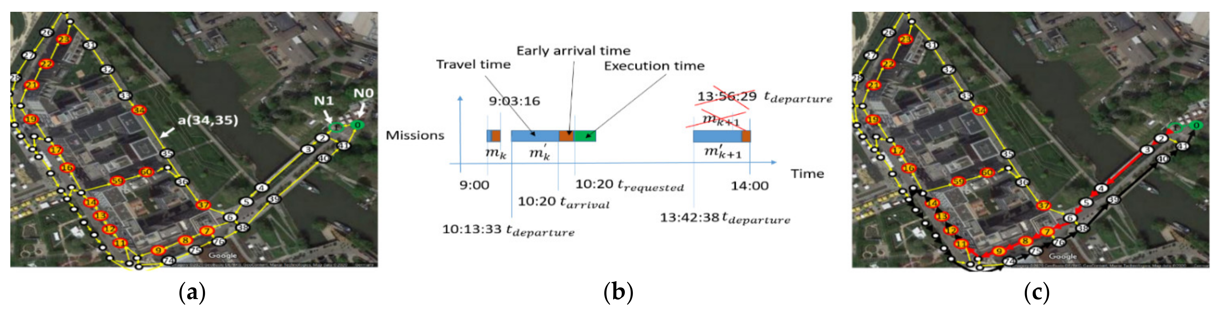
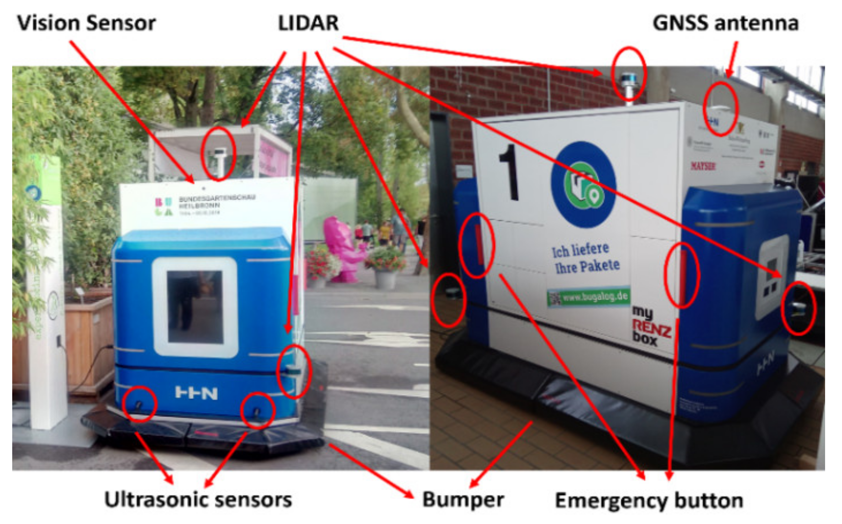
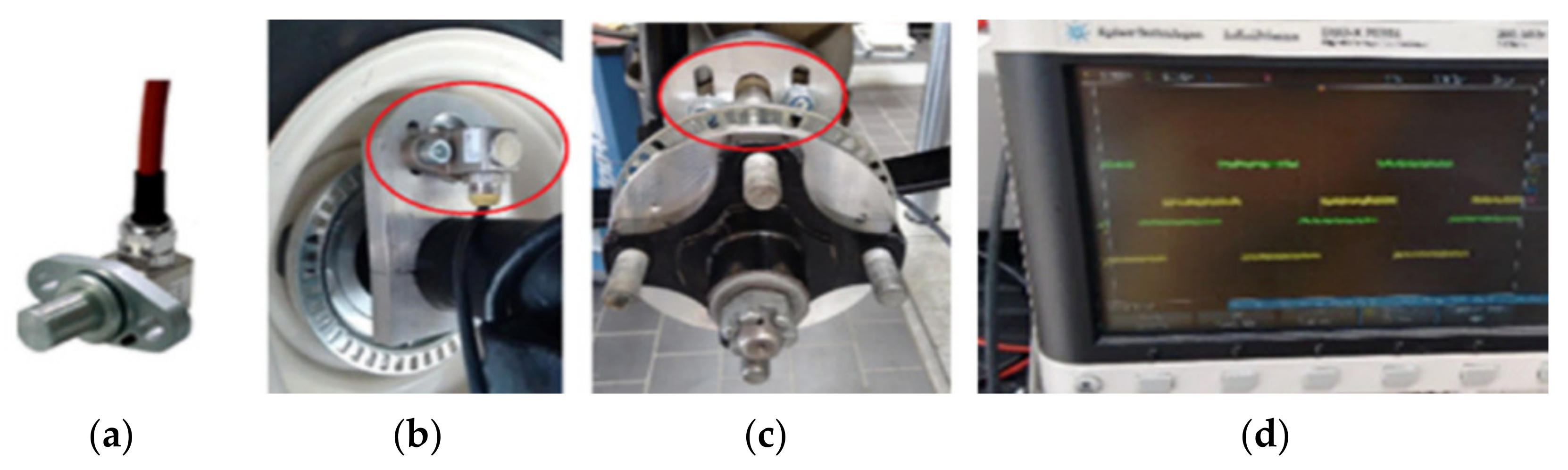
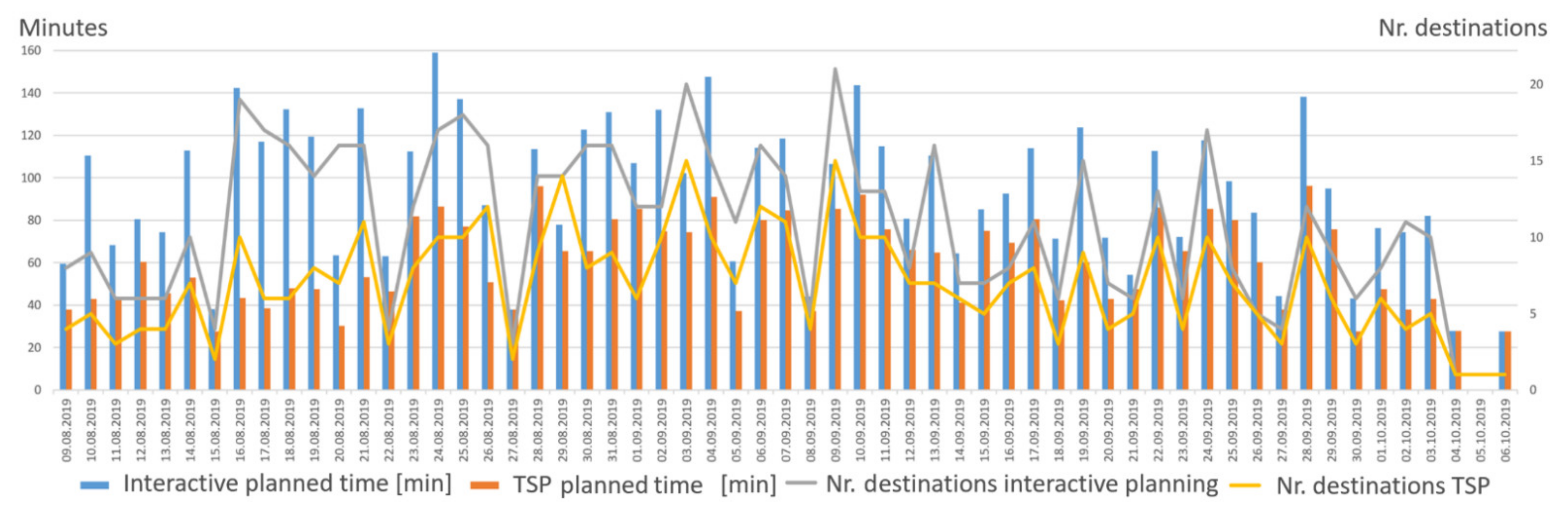
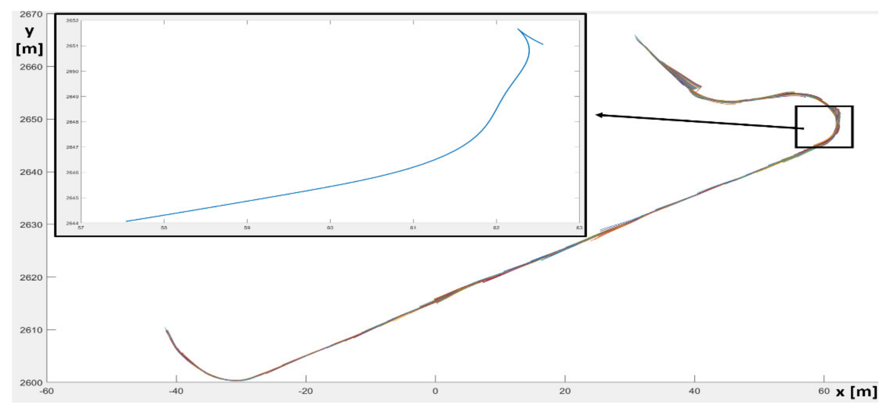
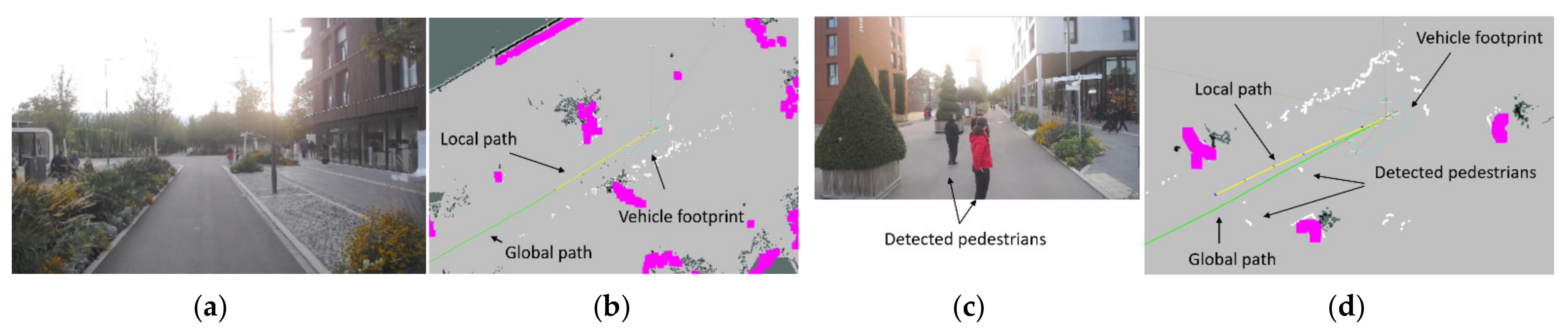
Table 1.
Process equations with uncertainty.
| Parameter | Equation | Uncertainty |
|---|---|---|
Table 2.
Maximal variance of the measured parameters used in the uncertainty matrix of the measurement process.
Table 2.
Maximal variance of the measured parameters used in the uncertainty matrix of the measurement process.
| Measured | Maximal Variance |
|---|---|
Table 3.
Extract of risks and safety measurements according to ISO26262.
| Code | Risk Description | Safety Measurement |
|---|---|---|
| R01 | The autonomous vehicle does not detect obstacles | Use-certified bumper system with redundant ultrasonic sensors |
| R02 | The autonomous vehicle does not stop | Placement of emergency buttons accessible on each side of the vehicle |
| R03 | The operating speed exceeds the 6 km/h speed restriction | Speed restriction from certified motor controller of the golf cart, as well as software restriction |
| R04 | Failure of the braking system | Periodic check |
| R05 | The autonomous vehicle leaves the operating area | Fencing of the operating area |
| R06 | Uncontrolled acceleration of the autonomous vehicle | Use-certified bumper system with redundant ultrasonic sensors Placement of emergency buttons accessible on each side of the vehicle |
| R07 | Uncontrolled direction change of the autonomous vehicle | Use-certified bumper system with redundant ultrasonic sensors Placement of emergency buttons accessible on each side of the vehicle |
| R08 | The autonomous vehicle continues to move after an emergency stop, triggered by non-certified components | Use-certified bumper system with redundant ultrasonic sensors Placement of emergency buttons accessible on each side of the vehicle |
Table 4.
Statistical punctuality data for deliveries with one operating slot a day (9–21 August).
| Requests/Delays/Cancellation | No. of Requests | Planned Requests (%) | Executed Requests (%) |
|---|---|---|---|
| Planned requests | 147 | 100 | - |
| Executed requests | 118 | 80.27 | 100 |
| Executed without delay | 78 | 53.06 | 66.10 |
| Total delays | 40 | 27.21 | 33.89 |
| Over 15 min delay | 1 | 0.68 | 0.84 |
| Between 10 and 15 min delay | 3 | 2.04 | 2.54 |
| Between 5 and 10 min delay | 2 | 1.36 | 1.69 |
| Between 3 and 5 min delay | 3 | 2.04 | 2.54 |
| Between 1 and 3 min delay | 14 | 9.52 | 11.86 |
| Under 1 min | 17 | 11.56 | 14.40 |
| Cancelled by the monitoring system | 16 | 10.88 | - |
| Picked by client, without informing the system | 12 | 8.16 | - |
| Cancelled due to a previous delay | 3 | 2.04 | - |
Table 5.
Statistical punctuality data for deliveries with two operating slots a day (22 August to 6 October).
Table 5.
Statistical punctuality data for deliveries with two operating slots a day (22 August to 6 October).
| Requests/Delays/Cancellation | No. of Requests | Planned Requests (%) | Executed Requests (%) |
|---|---|---|---|
| Planned requests | 484 | 100 | - |
| Executed requests | 454 | 93.8 | 100 |
| Executed without delay | 337 | 69.62 | 74.22 |
| Total delays | 117 | 24.17 | 25.77 |
| Over 15 min delay | 4 | 0.82 | 0.88 |
| Between 10 and 15 min delay | 7 | 1.44 | 1.54 |
| Between 5 and 10 min delay | 24 | 4.95 | 5.28 |
| Between 3 and 5 min delay | 17 | 3.51 | 3.74 |
| Between 1 and 3 min delay | 35 | 7.23 | 7.71 |
| Under 1 min | 30 | 6.60 | 6.20 |
| Cancelled by the monitoring system | 20 | 4.13 | - |
| Picked by client, without informing the system | 4 | 0.82 | - |
| Cancelled due to a previous delay | 6 | 1.23 | - |
Table 6.
Position deviation between EKF with all inputs (odometry, GNSS, and AMCL) and inputs with only odometry, odometry + GNSS, and odometry + AMCL.
Table 6.
Position deviation between EKF with all inputs (odometry, GNSS, and AMCL) and inputs with only odometry, odometry + GNSS, and odometry + AMCL.
| Method | Odometry (m) | Odometry + GNSS (m) | Odometry + AMCL (m) | |
|---|---|---|---|---|
| Deviation | ||||
| Minimum | 0.0251 | 0.0011 | 0.0024 | |
| Average | 1.1219 | 1.1219 | 0.3977 | |
| Maximum | 4.5958 | 4.5958 | 1.8525 | |
Publisher’s Note: MDPI stays neutral with regard to jurisdictional claims in published maps and institutional affiliations. |
© 2022 by the authors. Licensee MDPI, Basel, Switzerland. This article is an open access article distributed under the terms and conditions of the Creative Commons Attribution (CC BY) license (https://creativecommons.org/licenses/by/4.0/).
Share and Cite
MDPI and ACS Style
Kocsis, M.; Zöllner, R.; Mogan, G. Interactive System for Package Delivery in Pedestrian Areas Using a Self-Developed Fleet of Autonomous Vehicles. Electronics 2022, 11, 748. https://doi.org/10.3390/electronics11050748
AMA Style
Kocsis M, Zöllner R, Mogan G. Interactive System for Package Delivery in Pedestrian Areas Using a Self-Developed Fleet of Autonomous Vehicles. Electronics. 2022; 11(5):748. https://doi.org/10.3390/electronics11050748
Chicago/Turabian StyleKocsis, Mihai, Raoul Zöllner, and Gheorghe Mogan. 2022. "Interactive System for Package Delivery in Pedestrian Areas Using a Self-Developed Fleet of Autonomous Vehicles" Electronics 11, no. 5: 748. https://doi.org/10.3390/electronics11050748
Note that from the first issue of 2016, this journal uses article numbers instead of page numbers. See further details here.