An Analytical Approach to Calculate Soft Error Rate Induced by Atmospheric Neutrons

Abstract

In the atmosphere, it is generally understood that neutrons are the main contributor to the soft error rate (SER) in electronic devices. These particles are indeed able to trigger nuclear reactions in the sensitive regions of the devices, leading to secondary ions that may ionize the matter sufficiently to upset a memory cell or induce a transient signal, known as soft errors. For reliability purposes, it is crucial to be able to estimate the SER associated with a given technology, which is typically characterized by its sensitive volume and its threshold linear energy transfer (LET). As an alternative to the usual Monte Carlo methods, in this work we present an analytical model for SER prediction, where we separate the radiation–matter interaction from the geometry considerations (sensitive volume). By doing so, we show that the SER can be expressed as the sum of two contributions that can be calculated for any threshold LET and any sensitive volume size. We compare our proposed approach to existing Monte Carlo simulations in the literature, obtaining a very good agreement despite our approximations, thus validating our approach. As an additional result, we can show that, for future down-sized technologies that may be more sensitive to radiation effects, the contribution of neutrons in the 1–10 MeV energy range to the SER is expected to decrease.

1. Introduction

In avionic and ground-level applications, neutrons are a major concern in terms of triggering single-event effects (SEE). The rate of non-destructive SEEs, called the soft error rate (SER), depends on the flux of particles and on the sensitivity of the considered device (generally represented by a sensitive volume and a critical charge/energy [1,2,3]). For reliability assessments, it is crucial to have tools [1,2,3,4,5] that estimate the SER for a given environment and a given technology. Besides supporting the planning and data analysis of irradiation test campaigns, such predictive tools can also improve the design and development of hardening techniques to enhance the robustness of a device or circuit. There are plenty of tools that aim to perform such calculations, and generally the Monte Carlo method is a good way to account for the numerous scenarios that may occur when a neutron breaks up a nucleus in an electronic device. Despite being highly effective, such methods require complex information about the device (often unavailable) and often involve long computational times.

In this work, we aimed to derive an analytical method to provide a simple way to calculate the SER with a minimum number of input parameters. The analytical burst generation rate (BGR) model, initially proposed by Ziegler and Landford [1] and improved by Letaw and Normand [2] and later by Tosaka [3], is based on the energy deposition inside a sensitive volume. This approach was justified for large-scale devices for which the sensitive volume extension was longer than the range of the particles. Basically, it was assumed that the only contributors to soft error were the secondary ions produced inside the sensitive volume. The SER was thus proportional to the sensitive volume, with a multiplying factor called the BGR, which accounted for the nuclear processes during a neutron–matter interaction. In today’s technologies, this approximation is no longer valid, and we must consider that particles created outside the sensitive volume can travel into the device before triggering a soft error. Here, we focus on an analytical approach that separates the geometrical consideration (associated with the sensitive volume of the technology) from the nuclear physics. The latter can be treated independently of the device under examination, while the geometrical aspect can be simply treated analytically.

As electronic technologies shrink, the minimum neutron energy able to trigger an SEE decreases. This means that low-energy neutrons may have a significant role since they are very abundant in the atmosphere [6,7,8]. Our work also aimed to evaluate the contribution of neutrons in the 1–10 MeV energy range to the soft error rate (SER) and determine if there is a trend with downscaling. To do so, we performed calculations of the SER for different technologies, isolating the contribution of neutrons in the 1–10 MeV energy range.

2. General Methodology to Evaluate the Soft Error Rate (SER)

2.1. Soft Error Rate

The SER depends on the sensitivity of the device and the flux of particles that can trigger SEEs. Therefore, to estimate the SER we need to know the following:

• The SEE cross section, ${\sigma }_{SEE}\left(E\right)$, characterizing the device sensitivity, which is known to decrease when neutron energy decreases;
• The neutron energy spectrum, $\frac{d\phi }{dE}$, which characterizes the atmospheric environment. Notice that, because neutrons result from multiple collisions of particles in the atmosphere, their distribution can be considered approximately isotropic.

The SER can then be calculated as follows:

$$SER={\int }_0^{\infty }{\sigma }_{SEE}\left(E\right)\frac{d\phi }{dE}dE$$

(1)

2.2. Worst-Case Analysis

The SEE cross section, ${\sigma }_{SEE}\left(E\right)$, measures the probability for an SEE to occur in a device and is therefore a quantity that depends on the considered technology. Experimentally, the cross section of a neutron has an onset above 1 MeV and reaches a saturation value at a few tens of MeV. In the worst-case scenario, depicted in Figure 1, we consider that the cross section is zero below 1 MeV and equal to a constant value, namely ${\sigma }_{sat}$, above.

The International Electrotechnical Commission (IEC) standard [7] gives the avionic flux, $\frac{d\phi }{dE}$ (i.e., for an altitude of 12 km and a latitude of 45 degrees). The standard suggests dividing this flux by 300 to obtain the flux at ground level. In this work, we used this method to focus on ground-level applications. Therefore, we could calculate the SER for four different neutron energy ranges of interest:

• 1 MeV–10 MeV: this range is of main importance since the onset decreases below 10 MeV with device downscaling.
• 10 MeV–50 MeV: in this region, the cross section increased toward the saturation cross section, and results can be very different from one technology to another.
• 50 MeV–200 MeV: the cross section has reached the saturation value.
• Above 200 MeV: the cross section should also be at saturation, but experimental data generally do not exist since monoenergetic beams of neutrons are not available.

Based on the flux of the IEC standard (divided by 300), the contributions of these energy ranges to the SER were calculated using Equation (1). The results are given in

Table 1. Contribution of four main energy ranges to the SER in the framework of the worst-case analysis, i.e., with constant SEE cross sections for neutrons above 1 MeV. Calculations were made using the flux of the IEC standard divided by 300 to obtain the contributions at ground level.

Energy Range	SER (FIT/Mcell)	Contribution to Total SER
1 MeV–10 MeV	$8.37·{10}^{15}\times {\sigma }_{sat}$ (cm2)	44%
10 MeV–50 MeV	$3.94·{10}^{15}\times {\sigma }_{sat}$ (cm2)	21%
50 MeV–200 MeV	$2.51·{10}^{15}\times {\sigma }_{sat}$ (cm2)	13%
200 MeV–100 GeV	$4.20·{10}^{15}\times {\sigma }_{sat}$ (cm2)	22%
Total	$19.02·{10}^{15}\times {\sigma }_{sat}$ (cm2)	100%

. It is shown that in the worst case (defined by the assumption of a constant SEE cross section for neutrons above 1 MeV) the contribution of the 1–10 MeV energy range is only 44% of the total SER at ground level. Hence, even though the differential flux drastically increases at low energy (by more than an order of magnitude from 10 MeV down to 1 MeV), neutrons in this energy range do not represent the main contributors to SER. Moreover, knowing that the SEE cross section typically decreases with energy below 10 MeV, this contribution could be much smaller.

2.3. Further Analysis

In the previous section, we learned that the 1–10 MeV range can represent, in the worst case, 44% of the total SER. It is thus not the main contribution to SER but it is sufficiently relevant to require investigating this energy range in more detail. To better quantify the contribution of low-energy neutrons to the SER, we must include technological parameters and more precisely describe the interaction of neutrons with matter. This is the goal of the next sections.

3. Analytical Tool to Evaluate the SER

Soft error rates are often computed using Monte Carlo tools, which are powerful but require long computation times and are typically case-specific, not easily allowing the extraction of general trends. In this work, we investigated an analytical approach to determine if it is possible to obtain a simple formula giving the SER as a function of the representative parameters of the technology under study.

3.1. Soft Error Triggering Criterion

When a nuclear reaction occurs, many different secondary ions are produced, which can trigger a soft error. In the present work, we consider that an ion triggers a soft error if the following conditions are fulfilled:

• The ion must cross through the sensitive region of the device. The boundaries of this sensitive volume are not clearly defined, and, for the sake of simplicity, we consider that it is a sphere of radius R_S.
• The ion must deposit enough energy inside the sensitive volume. To fulfill this condition, we consider that the ion must reach the sensitive volume with an adequate LET, which is defined as the characteristic threshold LET of the device, noted LET_th.

3.2. Ion Generation Rate

To evaluate the rate at which ions are produced due to nuclear reactions induced by neutrons, we must know the geometry of the device and the materials. This information is generally not known, but we can consider, in a first approximation, that the device is mainly composed of silicon. Therefore, in the following calculations, we only consider nuclear reactions that occur on silicon though light elements (such as oxygen) that can introduce variation in the SER evaluation.

As the mean free path of neutrons is quite long (typically 20 cm in silicon), we can assume that the rate of secondary ion production in our electronic device is uniform. If we consider ions that are produced by neutrons with energy between E_n1 and E_n2, the generation rate $\mathrm{G}\left(A,Z,E_{ion}\right)$ of a secondary ion, characterized by its mass number A, its atomic number Z, and its energy E_ion, has an energy distribution given by Equation (2):

$$\frac{d\mathrm{G}\left(E_{n1},E_{n2};A,Z,E_{ion}\right)}{d{E}_{ion}}={\int }_{E_{n1}}^{E_{n2}}\frac{d{\sigma }_{ion}\left(E_n;A,Z,E_{ion}\right)}{d{E}_{ion}}\times \frac{d\varphi \left(E_n\right)}{d{E}_n}d{E}_n$$

(2)

where:

• $\mathrm{G}\left(E_{n1},E_{n2};A,Z,E_{ion}\right)$ is the generation rate of the ion, given per unit of time and per target silicon nucleus;
• $\frac{d{\sigma }_{ion}\left(E_n;A,Z,E_{ion}\right)}{d{E}_{ion}}$ is the differential nuclear cross section to produce an ion A, Z with an energy of E_ion in the device;
• $\frac{d\varphi \left(E_n\right)}{d{E}_n}$ is the differential neutron flux of the environment being considered.

Additionally, we can define the cumulative production rate that gives a production rate above a given energy (${\int }_E^{\infty }\frac{d{\sigma }_{ion}}{d{E}_{ion}}d{E}_{ion}$). As an example, Figure 2 plots the cumulative distribution obtained in the case of secondary silicon ions at ground level for the neutron energy ranges of 1–10 MeV and 1–200 MeV. These distributions were computed using the DHORIN code [9] with Equation (2). We calculated these generation rates for all kinds of secondary ions (with mass number A and atomic number Z) that can be produced during nuclear reactions induced by a neutron on a silicon atom target. They include all elements from hydrogen (Z = 1) to silicon (Z = 14), including various isotopes.

3.3. Probability to Reach the Sensitive Volume

If a given ion is produced at a distance, r, from the center of the sensitive volume, its probability, P_geom(r), to be emitted in the direction of the sensitive volume (whose radius is R_s) can be estimated by simple geometrical considerations. This is justified by the fact that, as neutrons are isotropic in the atmosphere, secondary ions are too. Therefore, the probability for an ion to be emitted toward the sensitive volume may be estimated by Equations (3) and (4) [10]:

$$P_{geom}\left(r\right)=1 if r<R_{S }$$

(3)

and:

$$P_{geom}\left(r\right)\approx \frac{1}{4}{\left(\frac{R_S}{r}\right)}^2 if r\ge R_S$$

(4)

3.4. Ion Range and Threshold LET

The range R(A, Z, E_ion) of a secondary ion is defined as the distance it can travel before being stopped. For a given ion in a given material, the range R(A, Z, E_ion) can be calculated, for example, with the SRIM code [11]. Even if an ion is emitted toward the sensitive volume, it will not reach the sensitive volume if its range is shorter than the distance to cover ($~r-R_S$), which translates to a minimum energy requirement for the ion. Moreover, the ion must reach the sensitive volume with an adequate LET (>LET_th) to have a chance to trigger a soft error, and since the LET decreases at high energies, this requirement also implies the presence of an upper limit on the ion energy. In summary, the ion energy must be between E₁ and E₂ such as $LET\left(E_1\right)=LET\left(E_2\right)=LE{T}_{th}$ and E₁ < E₂. This is illustrated in Figure 3.

Figure 3 shows a typical evolution of the LET as a function of its energy. It depends on the ion and the material that is crossed by the ion, but it always has this kind of peak, which is called a Bragg peak. We also represented a second x-axis to show the relationship between the ion energy, E_ion, and its range, R(A, Z, E_ion). We can see that, if an ion (with an energy E_ion) travels a distance that is too short (i.e., <R₂) before entering the sensitive volume, its LET will be lower than the threshold LET. Therefore, to trigger an event, it must cover at least the distance R₂. Similarly, if it covers a distance that is too long (longer than R₁), it will enter the sensitive volume with an energy lower than E₁, which corresponds to an LET below the threshold. Consequently, the distance ($~r-R_S$) traveled by the ion before reaching the sensitive volume must be between R₁ and R₂. In other words, the distance, r, at which the ion is produced from the center of the sensitive volume must obey Equation (5):

$$R_{min}\le r\le R_{max}$$

(5)

where R_min should obey Equations (6) and (7):

$$R_{min}=R\left(E_{ion}\right)+R_S-R\left(E_2\right) if E_{ion}>E_2$$

(6)

$$R_{min}=0 otherwise$$

(7)

and R_max should obey Equation (8):

$$R_{max}=R\left(E_{ion}\right)+R_S-R\left(E_1\right)$$

(8)

3.5. Probability to Trigger a Soft Error

The first condition for an ion (A, Z) to be able to trigger a soft error is that its LET at the Bragg peak is higher than the threshold LET of the considered technology. This may be written according to Equation (9):

$$\forall E_{ion}, P_{SEE}\left(A,Z\right)=0 if LE{T}_{max}\left(A,Z\right)<LE{T}_{th}$$

(9)

Otherwise, once generated with an energy, E_ion, the probability that an ion (A, Z) triggers a soft error depends on both the probability of being emitted toward the sensitive volume and the condition of r given by Equation (5). Therefore:

$$P_{SEE}\left(A,Z,E_{ion}\right)={\int }_{R_{min}}^{R_{max}}4\pi N_{Si}{P}_{geom}\left(r\right)r^{2}dr$$

(10)

where $N_{Si}$ is the number of silicon targets per unit volume ($N_{Si}=5\times {10}^{22} \mathrm{at}/{\mathrm{cm}}^3$).

Now, to calculate the integral of Equation (10), we need to consider two cases:

• If E_ion > E₂:

In this case, after Equation (6), we have R_min > R_S. This means that P_geom is given by Equation (4). Therefore, Equation (10) becomes Equation (11):

$$P_{SEE}\left(A,Z,E_{ion}\right)=\pi N_{Si}{R}_S{}^2\left(R\left(E_2\right)-R\left(E_1\right)\right)$$

(11)

• If E_ion < E₂:

Here, we have R_min < R_S, and we must distinguish ions that are produced inside and outside the sensitive volume. We thus split the integral into two parts, and Equation (10) becomes Equation (12):

$$P_{SEE}\left(A,Z,E_{ion}\right)={\int }_{R_{min}}^{R_S}4\pi N_{Si}{P}_{geom}\left(r\right)r^{2}dr+{\int }_{R_S}^{R_{max}}4\pi N_{Si}{P}_{geom}\left(r\right)r^{2}dr$$

(12)

which leads, using Equations (3) and (4), to Equation (13):

$$P_{SEE}\left(A,Z,E_{ion}\right)=\frac{4}{3}\pi N_{Si}{R}_S{}^3+\pi N_{Si}{R}_S{}^2\left(R\left(E_{ion}\right)-R\left(E_1\right)\right)$$

(13)

It is worth noting that the probability that an ion triggers a soft error is a third-degree polynomial of R_S in which the coefficients only depend on the threshold LET (included in E₁, as illustrated in Figure 3). In fact, the term with the power of 3 is linked to the sensitive volume, and the term with the power of 2 is linked to its surface.

3.6. Soft Error Rate

Finally, the soft error rate due to an ion (A, Z) generated by an atmospheric neutron in the [E_n1 ; E_n2] energy range and for a technology characterized by its sensitive volume radius, R_S, and its threshold LET is given as follows:

$$SER\left(E_{n1},E_{n2};A,Z;R_S,LE{T}_{th}\right)={\int }_{E_1}^{\infty }{P}_{SEE}\left(A,Z,E_{ion}\right)\times \frac{d\mathrm{G}\left(E_{n1},E_{n2};A,Z,E_{ion}\right)}{d{E}_{ion}}d{E}_{ion}$$

(14)

In Equation (14), the integral starts at E₁ since below this value there is no possibility to trigger a soft error. As the probability P_SEE has a different expression depending on the value of E_ion compared to E₂ (see Section 3.5), we split the integral into two parts

$$SER\left(E_{n1},E_{n2};A,Z;R_S,LE{T}_{th}\right)=I_V\left(E_{n1},E_{n2};LE{T}_{th}\right)\times \frac{4}{3}\pi R_S{}^3+I_S\left(E_{n1},E_{n2};LE{T}_{th}\right)\times \pi R_S{}^2$$

(15)

where I_V (volume term) and I_S (surface term) are two functions that only depend on LET_th and the considered energy range. They are defined as follows:

$$I_V\left(E_{n1},E_{n2};LE{T}_{th}\right)=N_{Si}{\int }_{E_1}^{E_2}\frac{d\mathrm{G}}{d{E}_{ion}}d{E}_{ion}$$

(16)

$$I_S\left(E_{n1},E_{n2};LE{T}_{th}\right)=N_{Si}\left\{{\int }_{E_1}^{E_2}\left(R\left(E_{ion}\right)-R\left(E_1\right)\right)\frac{d\mathrm{G}}{d{E}_{ion}}d{E}_{ion}+{\int }_{E_2}^{\infty }\left(R\left(E_2\right)-R\left(E_1\right)\right)\frac{d\mathrm{G}}{d{E}_{ion}}d{E}_{ion}\right\}$$

(17)

The main conclusion of this calculation is that we can obtain analytically the SER in a specific range of neutron energy and for a given technology characterized by Rs and LET_th. The main advantage is that we have separated the geometrical consideration (R_S) from the nuclear physics (I_V and I_S). The two quantities can be precomputed with a dedicated nuclear physics tool, and the SER is finally simply calculated using Equation (15).

4. Main Results and Discussions

4.1. Example of SER Calculation for 1–200 MeV

We calculated, with the DHORIN code, the functions I_S and I_V, which are plotted in Figure 4 for the 1–200 MeV energy range. Basically, the I_V function represents the nuclear reactions that occur inside the sensitive volume, while the I_S function represents those that are triggered outside the sensitive volume.

To show how we can calculate the SER, let us consider an arbitrary technology studied in work [3], which used an improved BGR model. In this work, the sensitive volume was known to have a value of 4.5 μm³ (corresponding, in our approach, to a radius of the sensitive volume of R_s = 1.02 μm) and a critical charge of 30 fC (corresponding to a threshold LET of 2.82 MeV·cm²/mg). From Figure 4, we can read that I_V = 200 FIT/Mcell/μm³ and I_S = 300 FIT/Mcell/μm². We can calculate the SER at ground level using Equation (15), which leads to Equation (18):

$$SER=200\times \frac{4}{3}\pi R_S^3+300\times \pi R_S^2=1880 \mathrm{FIT}/\mathrm{Mcell}$$

(18)

Notice that this value is in very good agreement with work [3], which was given to be 1900 FIT/Mcell. However, work [3] was given to deal with the critical charge down to 10 fC, while current technologies are known to be around 1 fC and even below.

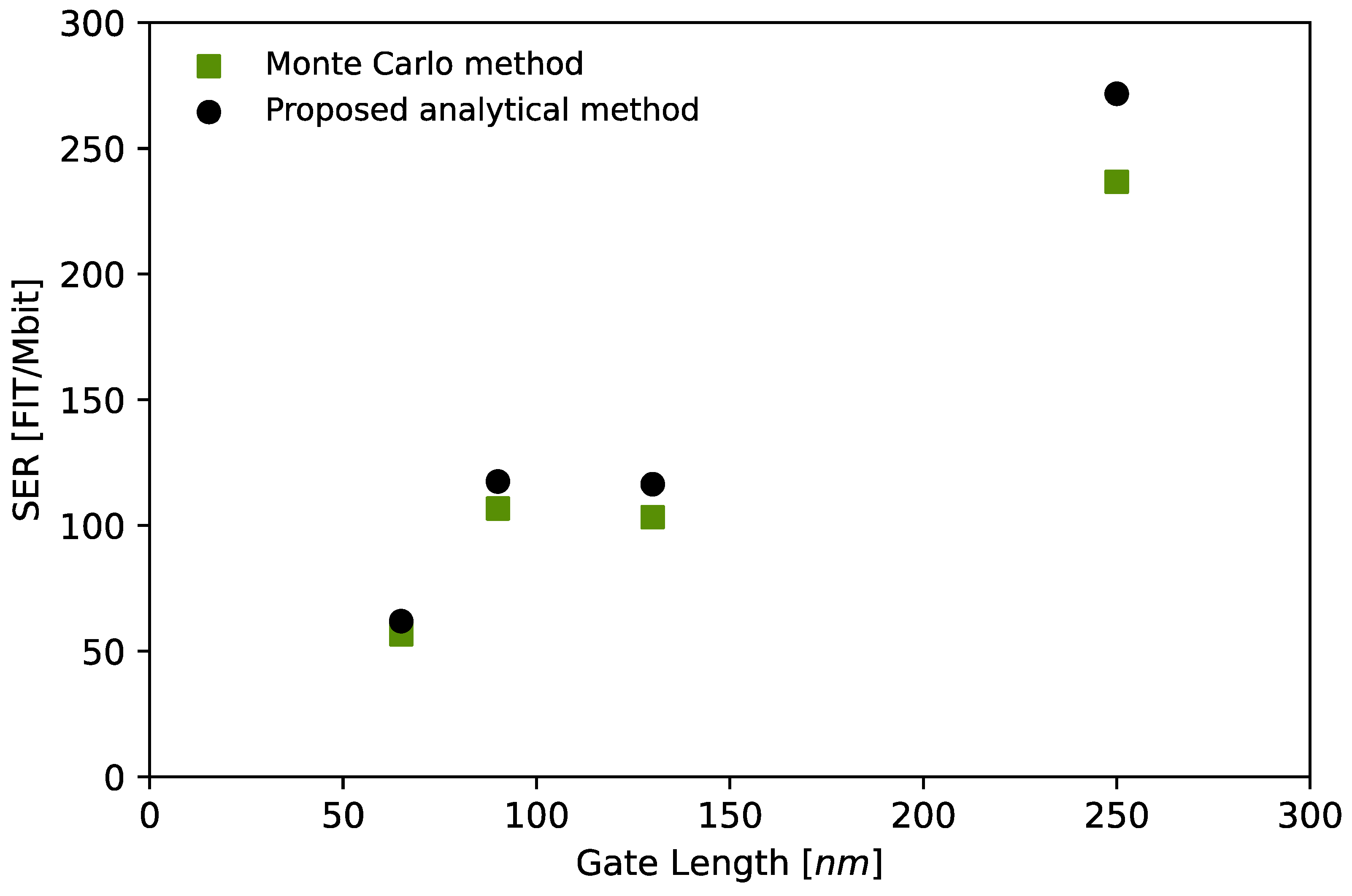
To validate our approach below 10 fC, we compared our results with Monte Carlo simulation results from the literature [12] based on some technology information [13]. These simulations used a cube for the sensitive volume, and we simply calculated the radius of a sphere with the same volume. Four technologies were studied, each with a different gate length (250 nm, 130 nm, 90 nm, and 65 nm). For each of them, the critical charge was known, and the threshold LET could be estimated by dividing this charge by the radius of the sensitive volume (with the appropriate unit conversion).

Table 2. Comparison of SER at ground level between the Monte Carlo method and the presented method.

Gate Length (nm)	Sensitive Volume (μm3)	Rs (μm)	Qc (fC)	LETth (MeV·cm2/mg)	SER Monte Carlo at Ground Level (FIT/Mbit)	IS (FIT/Mcell/μm2)	IV (FIT/Mcell/μm3)	SER (Equation (15)) at Ground Level (FIT/Mcell)
250	0.245	0.388	8	1.99	237	380	380	272
130	0.025	0.181	2.5	1.34	103	913	913	116
90	0.01	0.134	1.2	0.87	107	1850	1323	117
65	0.0035	0.094	0.8	0.82	56.7	2068	1330	62

gives the relevant parameters, the SER calculated by the Monte Carlo method, and the SER calculated using Equations (15)–(17). The comparison of the SER obtained by the two approaches is plotted in Figure 5. The difference between the two approaches was lower than 13%, despite the differences in terms of modeling and the approximations made in this work. It must be noted that our method systematically overestimates the SER compared to the Monte Carlo method, which is fine for reliability purposes (worst case). Moreover, the fact that this difference slightly decreases with downscaling is not well understood but is due to our approximations.

4.2. I_V Calculation for 1–10 MeV

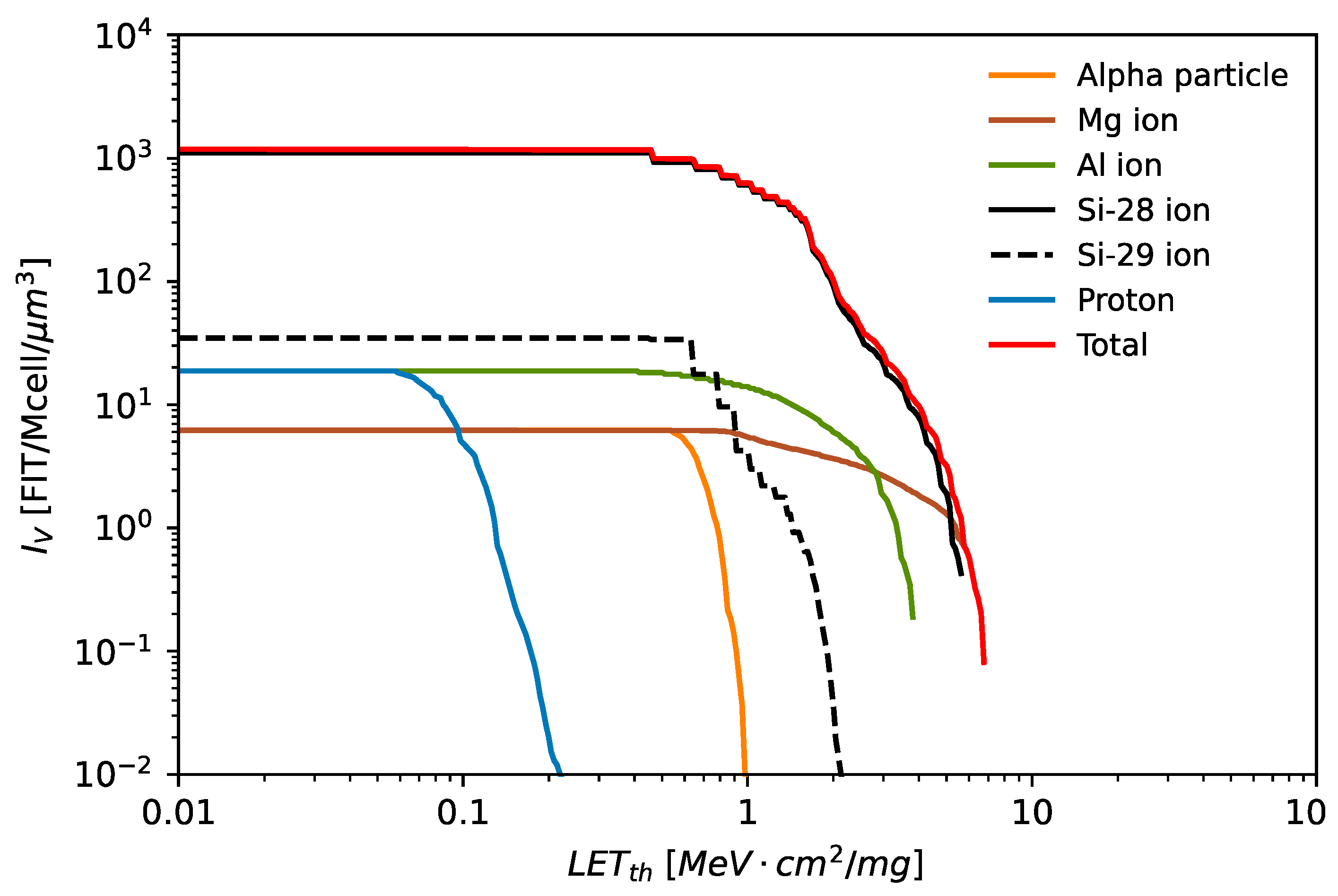
For the 1–10 MeV neutron energy range, we calculated, using the DHORIN code, the term I_V, associated with the sensitive volume, and we plotted the contribution of each secondary ion as a function of the threshold LET. The results are shown in Figure 6. It appears that the main contribution was due to the recoiling silicon ions (from elastic and inelastic reactions), except for at very high LET_th values, where the Mg ion contribution was dominant.

For modern technologies, where the threshold LET is typically between 0.1 and 1 MeV·cm²/mg, I_V is in the range of 600–1100 FIT/Mcell/μm³. For very sensitive technologies that are even sensitive to direct ionization from protons, the threshold LET is below 0.54 MeV·cm²/mg. For all these technologies, I_V no longer depends on the LET_th. Consequently, this means that this first contribution to the SER is only governed by the size of the sensitive volume. With downscaling, this contribution is then expected to decrease, ultimately becoming negligible. Concerning light particles (proton and alpha) produced in the neutron-induced reaction, their contribution is negligible since they must be produced at the Bragg peak inside the sensitive volume, which is more and more unlikely with transistor scaling.

4.3. I_S Calculation for 1–10 MeV

We calculated, with the DHORIN code, the term I_S, which is associated with the visible surface of the sensitive volume and plotted the contribution of each secondary ion as a function of the threshold LET. The results are shown in Figure 7. Above 1.45 MeV·cm²/mg, the main contribution was again attributed to recoiling ²⁸Si and ²⁵Mg. However, below 1.45 MeV·cm²/mg, the light particles (proton and alpha) had a role since they were produced outside the sensitive volume and may have reached it with a sufficient LET. This is the reason why the I_S function increased more rapidly below 1.45 MeV·cm²/mg (alpha contribution) and even more below 0.54 MeV·cm²/mg (proton contribution).

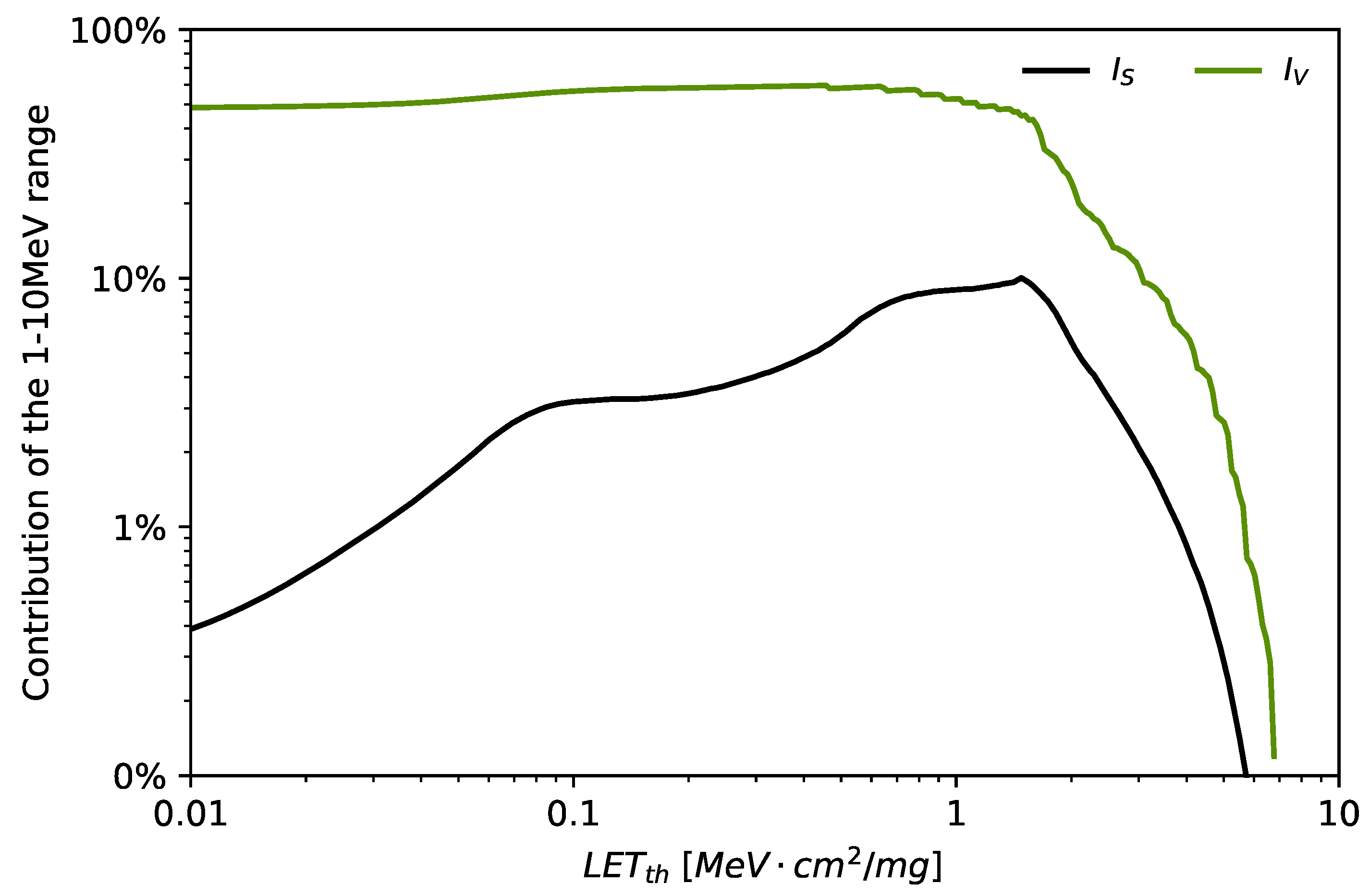
4.4. Contribution of the 1–10 MeV Energy Range to the SER

We investigated the contribution of the 1–10 MeV neutron energy range to the total SER (at ground level). To do so, we used Equation (17) to calculate I_S (E_n1 = 1 MeV, E_n2 = 10 MeV) and I_S (E_n1 = 1 MeV, E_n2 = 200 MeV). Dividing the first quantity by the second one led to the contribution of the 1–10 MeV range to the I_S term. Similarly, using Equation (16) allowed us to evaluate the contribution to the I_V term. The results are presented in Figure 8. For the I_V function, the contribution of the 1–10 MeV energy range increased when the LET_th was decreasing (which corresponds to device downscaling). For LET_th < 1.5 MeV·cm²/mg this contribution was quite constant, showing that there was a limitation of the low-energy range when shrinking the device. As far as the I_S function is concerned, the contribution of the 1–10 MeV energy range decreased for LET_th < 1.5 MeV·cm²/mg, meaning again that downscaling will not indefinitely increase the contribution of low-energy particles.

In summary, for down-sized technologies with low threshold LET values, the observation that the contribution of 1–10 MeV to I_V is constant and the contribution to I_S is decreasing implies that the overall contribution of this energy range to the SER is decreasing.

5. Conclusions

In this work, we examined neutron-induced SEEs and developed an analytical model aimed at calculating the SER, which also allowed us to investigate the contribution of low-energy neutrons (1–10 MeV). To build an efficient tool, we separated the radiation–matter interaction from the geometry considerations (sensitive volume). It is generally assumed that an SEE occurs when an ion crosses the sensitive volume and releases enough energy. We slightly modified this assertion by considering that it is equivalent to reaching the sensitive volume with an adequate LET (called LET_th).

The probability that an ion reaches the sensitive volume was computed analytically. On the other end, the nuclear physics part was calculated with the DHORIN code, which allowed us to determine the energy distributions of all secondary ions that can be produced, from hydrogen (Z = 1) to silicon (Z = 14), including their isotopes. Two main functions were derived: I_V(LET_th), which is related to the nuclear reactions occurring inside the sensitive volume, and I_S(LET_th), which is related to those occurring outside the sensitive volume. We found very good agreement between our results and Monte Carlo simulations of SER from the literature. We investigated the 1–10 MeV and the 1–200 MeV energy ranges, and we showed that, with the downscaling evolution, the contribution of the lowest energy range is not expected to increase, even if the sensitivity is increasing (as expressed by the decreasing LET_th).

In this work, we focused on low-energy neutrons in the atmosphere, but the methodology can be replicated for other environments such as accelerators. To do so, we need to know the neutron spectra and need to compute the associated ion generation rate using a code such as DHORIN or an equivalent. Then, the I_V(LET_th) and I_S(LET_th) functions can easily be calculated, and the contribution of the considered energy range to the total SER can be evaluated.

With device downscaling, electronic devices are more and more sophisticated, with many materials and complex geometries. It is crucial to perform accurate Monte Carlo simulations accounting for all these parameters. However, many of these parameters are proprietary, and it is necessary to develop calculation methods that rely on less parameters. This kind of method, including the method presented here, can be used by any end-user of an electronic device and with very short calculation times (less than a minute, compared to a Monte Carlo simulation that can last hours or even days).

Finally, it seems possible to account for other kinds of materials if the geometry remains simple (i.e., the addition of different layers of materials). Our approach could also be extended to the proton environment that is encountered in space.

References

- Ziegler, J.F.; Lanford, W.A. Effect of Cosmic Rays on Computer Memories. Science 1979, 206, 776–788. [Google Scholar] [CrossRef] [PubMed]
- Letaw, J.R.; Normand, E. Guidelines for predicting single-event upsets in neutron environments. IEEE Trans. Nucl. Sci. 1991, 36, 2348. [Google Scholar]
- Tosaka, Y.; Kanata, H.; Satoh, S.; Itakura, T. Simple method for estimating neutron-induced soft error rates based on modified BGR model. IEEE Electron Device Lett. 1999, 20, 89–91. [Google Scholar] [CrossRef]
- Connell, L.; Sexton, F.; Prinja, A. Further development of the Heavy Ion Cross section for single event UPset: Model (HICUP). IEEE Trans. Nucl. Sci. 1995, 42, 2026–2034. [Google Scholar] [CrossRef]
- Reed, R.A.; Weller, R.A.; Akkerman, A.; Barak, J.; Culpepper, W.; Duzellier, S.; Foster, C.; Gaillardin, M.; Hubert, G.; Jordan, T.; et al. Anthology of the Development of Radiation Transport Tools as Applied to Single Event Effects. IEEE Trans. Nucl. Sci. 2013, 60, 1876–1911. [Google Scholar] [CrossRef]
- Measurement and Reporting of Alpha Particle and Terrestrial Cosmic ray-Induced Soft Errors in Semiconductor Devices. JEDEC Solid State Technology Association, Sept. 2021. Available online: https://www.jedec.org/standards-documents/docs/jesd-89a (accessed on 26 November 2022).
- IEC/TS 62396-1; Process Management for Avionics–Atmospheric Radiation Effects–Part 1: Accommodation of Atmospheric Radiation Effects via Single Event Effects within Avionics Electronic Equipment. IEC: Geneva, Switzerland, 2006.
- Quinn, H.; Watkins, A.; Dominik, L.; Slayman, C. The Effect of 1–10-MeV Neutrons on the JESD89 Test Standard. IEEE Trans. Nucl. Sci. 2019, 66, 140–147. [Google Scholar] [CrossRef]
- Wrobel, F. Detailed history of recoiling ions induced by nucleons. Comput. Phys. Commun. 2008, 178, 88–104. [Google Scholar] [CrossRef]
- Wrobel, F.; Palau, J.M.; Iacconi, P.; Palau, M.C.; Sagnes, B.; Saigné, F. Methodology to compute neutron-induced alphas contribution on the SEU cross section in sensitive RAMs. IEEE Trans. Nucl. Sci. 2004, 51, 3291–3297. [Google Scholar] [CrossRef]
- Ziegler, J.F. TRIM96. The TRansport of Ions in Matter. IBM-Research. 1996. Available online: http://www.srim.org/ (accessed on 26 November 2022).
- Wrobel, F.; Iacconi, P. Parameterization of neutron-induced SER in bulk SRAMs from reverse Monte Carlo Simulations. IEEE Trans. Nucl. Sci. 2005, 52, 2313–2318. [Google Scholar] [CrossRef]
- Roche, P.; Gasiot, G.; Forbes, K.; O’Sullivan, V.; Ferlet, V. Comparisons of soft error rate for SRAMs in commercial SOI and bulk below the 130-nm technology node. IEEE Trans. Nucl. Sci. 2003, 50, 2046–2054. [Google Scholar] [CrossRef]