
A Multi-Objective Approach to Robust Control of Air Handling Units for Optimized Energy Performance

1
Department of Electrical, Computer & Software Engineering, The University of Auckland, Auckland 1010, New Zealand
2
SKEMA Business School, Université Côte d’Azur, Sophia Antipolis, 06108 Nice, France
*
Author to whom correspondence should be addressed.
Electronics 2023, 12(3), 661; https://doi.org/10.3390/electronics12030661
Submission received: 27 December 2022
/
Revised: 24 January 2023
/
Accepted: 26 January 2023
/
Published: 28 January 2023
(This article belongs to the Special Issue Resource Sustainability for Energy and Electronics)
Abstract
:This paper presents a robust control framework with meta-heuristic intelligence to optimize the energy performance of air handling units (AHUs) and to maximize the thermal comfort of occupants by judiciously selecting the temperature set points of two controllers (i.e., the controller and the boiler controller). The selection of these set points is formulated as a multi-objective optimization problem, where the goal is to balance energy consumption with thermal comfort. Furthermore, the uncertainty weights of the controller are estimated to minimize oscillations in the outflow air temperature of the AHU plant. The performance of the proposed framework is investigated by considering the real-time weather data of Auckland, New Zealand. The results of the simulation show that the proposed robust control framework could significantly reduce oscillations in the outflow air temperature compared with the conventional case, where the temperature set points are selected empirically. Moreover, annual energy savings of are achieved without compromising the thermal comfort.
1. Introduction
The demand for energy consumption has been increasing at an alarming rate with the increase in world population. To meet this increasing energy demand, a large dependence of the world over the past decade or so has been non-renewable energy resources. This trend is more likely to remain the same in the foreseeable future, even though heavy investments are currently being made in the renewable energy sector. The complication is that the availability of non-renewable resources is scarce. The rate at which they are being consumed presently will make them insufficient for the increasing energy demand in the future. Moreover, their increasing use is also posing a detrimental impact on the Earth’s environment, which includes climate change (global warming), rising sea levels and so on. To become independent from the use of non-renewable resources seems to be feasible. However, this will not be dynamic, as it would take several decades to free ourselves from the use of non-renewable energy resources and completely switch to renewable energy resources [1]. Meanwhile, efficient utilization of the available energy resources can be regarded as a highly capable substitute to address the aforementioned problems, as this will prompt a reduced rate of non-renewable resource consumption [2]. The latest statistical data released by U.S Energy Information Administration (EIA) indicates that over of the energy produced from the world’s resources is consumed by the buildings sector alone, with residential and commercial buildings included, and more than one-third of this energy consumed is utilized for space heating and cooling [3,4]. These statistics give a strong implication that minimizing the energy usage of heating, ventilation and air conditioning (HVAC) systems can be a principal element in realizing the curtailment of world’s energy consumption and, consequently, global climate change. A need for optimizing the operation of HVAC systems is thus certain in order to minimize their overall uptime and energy consumption in buildings, but this should be realized such that the thermal comfort of the occupants is minimally affected. Maintenance of a comfortable environment for occupants is critically acknowledged as one of the important goals in smart and energy-efficient buildings [5,6]. Some of the factors which are fundamental in realizing the occupants’ overall comfort in a building environment include thermal comfort, air quality and visual comfort [7]. Realization of improvement in any of these comfort factors results in higher building energy consumption. One of the principal issues in building energy management systems (BEMS) is therefore to create a balance between two objectives: occupants’ thermal comfort and energy consumption.
In the past few decades, several useful energy management systems (EMS) have been proposed for optimized energy performance and thermal comfort management in buildings [7] using various control methods such as model predictive control (MPC) [8] and robust control [9]. In order to guarantee thermal comfort to the occupants, it is necessary to ensure minimal oscillations in the heating, ventilation and air conditioning (HVAC) plant output so that the desired set point values can be realized within stipulated time steps [10]. To this end, controllers based on modern control methods, such as , have been used in the past in HVAC control applications [11,12,13]. For instance, in [11], Underwood designed an -based robust controller for an HVAC plant by considering the nominal linear model, wherein the focus is on minimization of the oscillations in the outflow air temperature of the plant. Although the controller proposed in [11] performs well under design load conditions, it manifests oscillatory behavior in half and quarter load conditions. Such performance is often undesirable from both the thermal comfort and energy consumption points of view.
The controllers discussed above are essentially based on the concept of classical feedback control. It has been acknowledged that in order to have an effective thermal control system (strategy) in buildings, it should account for both of the above objectives (i.e., thermal comfort and energy consumption) simultaneously under all operating conditions [14,15]. To address this issue, many researchers in the area of smart BEMS have formulated the problem from a multi-objective optimization (MOO) perspective [16,17,18,19,20] where, in general, the concept of classical feedback control is integrated with heuristics. For instance, Jindal et al. [19] proposed an energy management scheme for controlling the HVAC systems in the classrooms of a university building, wherein a heuristic algorithm was proposed to optimally schedule the usage of HVAC. The results of the work indicated a reduction in the energy demand by HVAC systems for an entire week without affecting the thermal comfort of the occupants. However, the nonlinear nature of the HVAC system was not taken into account. In [10], the problem of maximizing the energy efficiency of HVAC systems was formulated as a nonlinear optimization problem and solved using the particle swarm optimization (PSO) technique. Wang et al. [20] proposed a multi-agent framework with heuristic intelligence for optimizing the overall occupant comfort and energy consumption in buildings. However, the influence of varying weather conditions, which are often responsible for causing heavy oscillations in an HVAC system’s output, was not considered. Some other recent research where multi-objective techniques have been utilized with a focus on HVAC systems in particular can be found in [21,22,23,24,25]. For instance, in [22], a convex programming (CP)-based DR optimization framework is presented for the load management of various household appliances through BEMS in a smart home. This work primarily targets the objectives which focus on optimizing the energy performance of HVAC systems. A multi-objective mixed-integer linear programming (MOMILP)-based framework was proposed in [24] to minimize building energy consumption. Furthermore, Li et al. [25] formulated an MOO problem for minimizing the operational costs of the utility, along with maximizing DR aggregators’ and users’ benefits. All the research mentioned and discussed above address very significant aspects of energy and comfort management in buildings. However, relatively less evidence could be found in the literature, where the nonlinear nature of the HVAC system model is considered along with focus on the balancing of energy consumption and comfort.
In the present study, a novel robust control framework is proposed which focuses on optimization of the energy performance of an air handling unit (AHU) while maintaining better occupant thermal comfort. This is achieved by effectively controlling the outflow air temperature of the AHU via two different controllers: an controller and a boiler controller. The performance of these controllers is critically determined by the set points (reference signals). Therefore, in the proposed framework, the selection of these set points to the controllers is formulated as a multi-objective optimization problem, wherein the goal is to balance the energy consumption of the AHU with the thermal comfort. In the optimization process, the optimal set points to these controllers are computed (in accordance with the occupant’s specified comfort parameters) using a well-known meta-heuristic: NSGA-II [26,27,28]. Some highlights of the proposed framework and main contributions of this paper are summarized as follows:
- 1
- A key aspect of our framework is that the multi-objective optimization is performed online, (i.e., the optimal set points are computed while considering the time-varying weather data of Auckland, New Zealand in real time during the simulations).
- 2
- To reduce the computation time per time step and to expedite the online optimization process, an approximation scheme is developed to estimate the water mass flow rate (an important variable in one of the objective functions). This reduces the complexity of the proposed framework as well.
- 3
- 4
- During the optimization process, an a posteriori approach is used to select the knee point solution from the pool of evaluated non-dominated optimal solutions. This ensures a proper balance between minimization of energy consumption and maintenance of thermal comfort.
- 5
- The uncertainty weights of the controller are estimated to reduce oscillations in the outflow air temperature of the AHU plant.
The remainder of this paper is organized as follows. Section 2 provides a brief description of the AHU plant model considered in this study. Section 3 explains the problem formulation. The structure of the control system is discussed in Section 4, followed by the simulation results and conclusions in Section 5 and Section 6, respectively.
2. Dynamic Model of the AHU Plant
The dynamics of the AHU plant (see Figure 1) derived from the first principles and considered in this study are given by [29].
Assuming an instantaneous heat transfer between the air and the heating coil, we have
where denotes the air mass flow rate, is a constant (1.002 kJ·kg·K) denoting the specific heat capacity of air and represents the inflow air temperature.
The thermal transfer coefficient on the water side of the coil for the turbulent-forced convection (heavy thermal load) is given by
and for the laminar forced convection (light thermal load), we have
Equations (4) and (5) represent a sharp edge, but the transition between the turbulent and laminar flow of liquid is gradual. For this purpose, the transition between the two has been relaxed as follows:
The thermal transfer coefficient on the air side of the coil is given by
Furthermore, assuming that the hysteresis due to the actuator linkage mechanism is negligible within the control valve, the mass flow rate of the water flowing through the coil can be represented as follows:
where
Since equal percentage characteristics are assumed for the control valve, we have
A first-order representation is also assumed for the temperature sensor:
3. Problem Formulation
The present study proposes a meta-heuristic based framework for robust control of the outflow air temperature of a typical AHU plant (see Figure 1). Herein, the prime goal is to achieve two objectives simultaneously: (1) minimization of AHU plant energy consumption by reducing the thermal load on the AHU and (b) maximization of thermal comfort by reducing the oscillations in the AHU plant output . To this end, two different controllers, an controller and a boiler controller, are used to control the outflow air temperature of the AHU plant (discussed in Section 4). The performance of these controllers is critically determined by the reference signals (set points) and . Therefore, the goal in this work is to determine the optimal values of these reference signals using a suitable multi-objective optimization technique such that the above two conflicting objectives are balanced.
Let us consider the pth solution set :
where and are being used to represent and , respectively, for the sake of simplicity. The superscript p represents the pth candidate solution set (particle) from the optimization technique (PSO) used in this paper. Hence, denotes the candidate outflow air temperature set point, and denotes the candidate inflow water temperature set point. These form the decision variables in the optimization process. The goal of the optimization task is to evaluate the optimal solution set (i.e., ) as shown below:
where represents the search domain of the decision variables to be specified by the decision maker (occupant). The objective functions and are mathematically expressed as follows:
- Energy function:where is an occupant-specified parameter (to be called the energy index) which determines the amount of thermal load on the AHU plant. It is worth emphasizing here that the energy consumption of the AHU plant is determined by the thermal load, which is influenced by the difference between the outside temperature and the set-point (i.e., ). Thus, the smaller this temperature difference, the smaller the thermal load on the AHU plant is.
- Discomfort function:The corresponding comfort level is calculated as follows:For the above expression of , refer to Section 3.1. Note that the occupants’ thermal discomfort is determined by the difference between the outflow air temperature and the set point . As this temperature difference decreases, the discomfort level of the occupants decreases (i.e., the comfort level increases).
For the pth candidate’s solution, at the kth time step (i.e., ), the objective functions and are evaluated as per Algorithm 1. It should be noted that for better functionality of the method, both objectives and are normalized (see Algorithm 1 (Line 11)).
| Algorithm 1: Evaluation of objective functions at the kth time step. |
Input: Search Agent, ; Outside Weather Profile, ; Energy Index, , AHU Plant Output, Output: Objective values: and */ Outside Sensor (temperature) data 1 Collect the outside temperature value, i.e., */ Evaluate the Objective Functions */ Intuitive energy consumption level 2 */ Approximate Mass-flow Rate, 3 Calculate error (see Figure 2); */ Compute Robust Controller Output, 4 fort = to do 5 6 end 7 8 */ Approximate 9 */ Occupant discomfort level, 10 */ Normalize and between 11; |
Figure 2.
Approximation approach to evaluating Equation (22).
Figure 2.
Approximation approach to evaluating Equation (22).
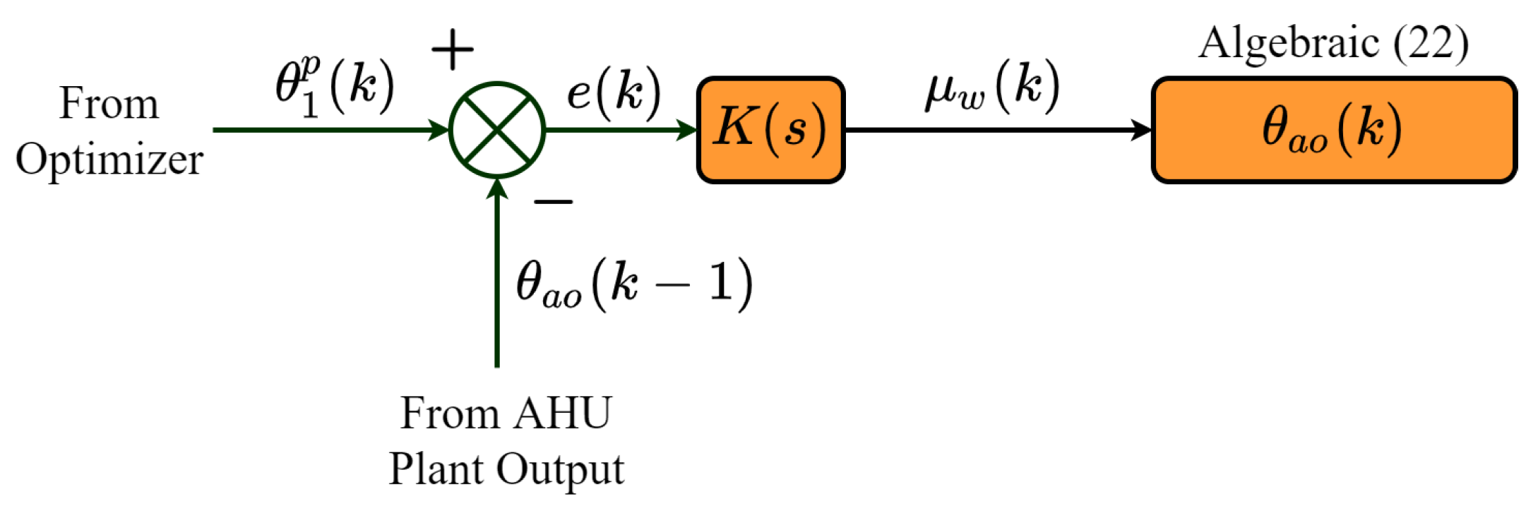
3.1. Approximation Approach to Evaluate
Since AHU plants are characterized by slower dynamics, it can be assumed at a given instant that
Based on this assumption, from Equation (1), we have
Under ideal conditions, it can be assumed that
For the pth solution set (i.e., )), we have
where = 4.194 kJ·kg·K, = 1.002 kJ·kg·K and = 0.3144 kg·s are all constants.
It is worth mentioning here that the ideal goal of the optimization task is to minimize and . However, these objectives are conflicting and cannot be minimized simultaneously in practice. Therefore, the goal is to search for the best possible solution which balances (satisfies) both objectives (energy function) and (discomfort function).
To this end, the framework comprises the following two processes.
3.2. Search Process
The principal step in the optimization process is to formulate an effective search strategy to find the optimal solution set, which in this case is (see Equation (13)). In this study, a multi-objective evolutionary algorithm (MOEA) called Non-Dominated Sorting Genetic Algorithm II (NSGA-II) is used for this purpose because of its popularity and efficiency in solving multi-objective optimization problems. NSGA-II is a seminal dominance-based MOEA which utilizes dominance-based relations for ranking and segregating the entire population of solutions into successive fronts using a well-known non-dominated sorting operation. Implementation and other details pertaining to NSGA-II are out of the scope of this paper and can be found elsewhere [31,32]. Although there are several multi-objective evolutionary algorithms (MOEAs) which are suitable for the task, such as Multi-Objective Particle Swarm Optimization (MOPSO), the Pareto Archived Evolution Strategy (PAES) and the Strength Pareto Evolutionary Algorithm (SPEA), this study considered the use of Non-Dominated Sorting Genetic Algorithm -II (NSGA-II). The rationale behind utilizing NSGA-II in this work is that it has been proven to perform well for solving multi-objective optimization problems (MOOPs) [33]. Further, NSGA-II is also known to be computationally better than its previous version (i.e., NSGA), apart from being able to give comparable performance to that of its two contemporary MOEAs (i.e., PAES and SPEA) [32,34].
In the framework, each search agent in NSGA-II represents a candidate solution set , the performance of which is evaluated as per the steps outlined in Algorithm 1. Note that the optimization process is performed online, and therefore for the pth candidate solution at the kth time step (i.e., ), the objective functions and are evaluated:
Due to the stochastic nature of NSGA-II, the best solution sets evaluated over multiple independent algorithm runs (denoted by R), are considered at every single time step k (see Algorithm 2 (Lines 2–5)).
| Algorithm 2: Meta-heuristic solution set selection. |
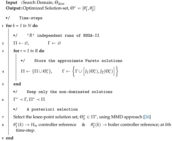 |
3.3. Best Solution Selection Process
After all the runs are complete, the non-dominated solutions over -runs are treated as the Approximate Pareto Front (APF) (i.e., ). Subsequently, the optimal set points and are selected from the APF by following the steps outlined in Lines 6 and 7 of Algorithm 2. Since the premise of this work is based on creating a balance between the above two objectives, an a posteriori selection approach called the minimum Manhattan distance (MMD) was adopted to select a knee point solution from the APF [26,27,28]. To this end, the Manhattan distance was determined between the hypothetical ideal point and each non-dominated solution in the APF . Following this, the solution corresponding to the minimum distance was selected:
where denotes the jth non-dominated solution in the APF . Finally, the identified knee point solutions (i.e., , ) are sent to the and the boiler controllers, respectively.
4. Structure of the Control System
The structure of the control system is shown in Figure 3. In particular, the two controllable inputs and of the AHU plant are controlled via the controller and the boiler controller, respectively. Moreover, to achieve the objectives described in Section 3, the system consists of an optimizer which has two parts: Part I and Part II. The purpose of Part I is to utilize the outside environmental information (i.e., the dry-bulb temperature ) collected by outside sensor and the occupant-specified comfort parameters to determine the optimal (best) temperature set point at each time step. This optimized set point is received by the controller, which controls the water mass flow rate flowing through the AHU coil by controlling the fractional valve-stem position F for temperature control. Part II of the optimizer focuses on controlling the inflow water temperature of the AHU plant. Note that the dead time (delay) between the inflow water temperature delivered by the boiler control system and the set point evaluated by our algorithm was assumed to be negligible (i.e., at a given time instant, ).
The design of the controller followed similar procedure to that given in [11], and it is therefore discussed briefly here for the sake of completeness.
Initially, the outflow air temperature of the AHU plant is generated via simulations from its nonlinear model (described in Section 2). The values of the parameters of the model used in the simulation can be found in [29]. A first-order lag plus delay linear time-invariant (LTI) model is fitted to this data:
The uncertainty bounds of various terms of the model in Equation (26) are determined by curve fitting and are given as [8.9 K, 48.4 K], [23.3 s, 41.3 s] and [47.9 s, 61.5 s]. Note that these bounds reflect the structural uncertainties of the model which are considered during the design of the controller.
The uncertainty in the gain () and time delay () parameters are used to derive the uncertainty weights, which consist of an integrator for performance () and first-order lead lag for the model uncertainty (), resulting in a fifth-order augmented plant description. Note that the controller weight () has been neglected in this design, the reason for which is explained well in [11]. The resulting augmented plant model is used to develop a robust controller (K) which minimizes the norm of the closed-loop plant (based on the solution of 2-Riccati algebraic equations), which is given as follows:
where S and T denote the normalized and complementary sensitivity functions, respectively. The transfer function of the stabilizing controller is given as
Note that in this work, the set point (i.e., ) varied after every 600 s as per the outside temperature (discussed in Section 5) . Thus, the purpose of the -based controller was to maintain stability and performance of the AHU in all operating conditions by regarding the varying optimal set point (i.e., ) as a disturbance.
5. Simulation Results and Discussion
The efficacy of the proposed framework in balancing the two conflicting objectives was investigated via simulations in a MATLAB®/Simulink® environment, considering the real-time weather profile of Auckland City. This was obtained from the meteorological data provided by the National Institute of Water and Atmospheric Research Limited (NIWA) in New Zealand [35].
5.1. Simulation Set-Up
The optimization was carried out online, where the objective functions and , corresponding to the pth candidate solution set at the kth time step (i.e., ), were evaluated as per Equations (23) and (24), respectively. Note that the value of the energy index was in the range of [0, 1]. In this work, is assumed to be one (i.e., minimizing the thermal load is assigned the highest priority).
The search domain used in this study is shown in Table 1. This was in compliance with the operative room temperatures recommended by the ASHRAE standard [36] (i.e., 20–23 °C during winter and 23–25 °C during summer). It is worth noting that the thermal comfort range (i.e., ) and the energy index were occupant (decision maker)-specified parameters and were key in evaluating the optimal (knee point) solutions (i.e., ) and (i.e., ).
The optimization was performed using the NSGA-II algorithm (see Section 3.2). To accommodate the stochastic nature of the NSGA-II algorithm, a total of 10 independent runs were carried out at each time step. Furthermore, single-point crossover was used as the recombination mechanism with the following crossover and mutation probabilities: . Each run of NSGA-II was terminated after 5000 function evaluations (FEs), and the population size was fixed at 50.
5.2. Performance Evaluation of the Controller without the Optimizer
Initially, the controller (described in Section 4) was designed to control the outflow air temperature by varying (see Figure 4). Without loss of generality, the investigation was carried out while considering both a notional periodic square waveform and a step signal as the reference (i.e., ) to the controller. Note that the AHU plant dynamics here were simulated for a duration of 4000 s (using square wave input) and 1000 s (using step input), respectively, at a sampling interval of . Furthermore, the reference of the boiler controller was chosen to be 28 °C. The output of the AHU plant () and the corresponding comfort level for these reference inputs are shown in Figure 5 and Figure 6 for three specific thermal load conditions. It was observed that the output of the AHU exhibited highly oscillatory behavior, particularly under part-load conditions, which resulted in a decreasing comfort level. Consequently, the power consumed by the AHU plant over a given duration also showed high oscillatory behavior with significant overshoots (see Figure 7 and Figure 8). Note that these observations are inline and consistent with the earlier investigations in [29], wherein similar oscillatory behavior was also observed under part-load conditions. Thus, the reference signals to the controller and the boiler controller shall be judiciously selected to achieve better comfort with less energy consumption.
5.3. Performance Evaluation of the Controller with the Optimizer
Following the simulation set-up described in Section 5.1 and the procedures explained in Section 3, the final output from the optimizer (i.e., the knee point solution(s) ), were used as reference signals for the controllers, which controlled the fractional valve-stem position , and the inflow water temperature of the AHU plant (see Figure 3). To supplement the understanding of this, Figure 9 and Figure 10 show the Pareto optimal fronts and the corresponding knee point solutions determined by our algorithm at four different outside temperatures .
It is worth mentioning that the AHU plant dynamics here were simulated while considering the Auckland weather profile data for the entire year (i.e., for a duration of 8640 h and with a sampling interval of 1 ms). Further, given that the slower dynamics tend to dominate the plant performance in HVAC system control, the set points were optimized at an interval of 10 min (i.e., the optimizer was operating at a step size of 600 s). For brevity purposes, we presented the performance of the controller with the proposed optimizer during a typical warm and a cool day in Figure 11 and Figure 12, respectively. Figure 11a shows the variation of optimized set points and , evaluated by the optimizer in accordance with the inflow air temperature (i.e., outside air temperature). It is worth noting that there was a huge fluctuation in the optimized inflow water temperature set point over time, particularly between 12:00 a.m. and 8:00 a.m. The reason for this was based on the working mechanism of the AHU plant (see Figure 1). In particular, the main variables which controlled the outflow air temperature were the fractional valve-stem position and the inflow water temperature . During the time between 12:00 a.m. and 8:00 a.m., the outside temperature was recorded to be the minimum, and as a result, the optimizer pushed the value of the optimized set point higher to keep the value of within the defined comfort range [19 °C, 25 °C] as per our proposed framework (see Table 1). Similar behavior can be observed in the trend of in Figure 12a, which was simulated for a day during the winter season. It can be observed that the controller with the optimizer (see Figure 3) was able to minimize the energy consumption compared with the controller without the optimizer (see Figure 4). Furthermore, this controller with the optimizer could maintain the occupant comfort at a higher level.
Note that to determine and compare the overall energy performance, the AHU plant dynamics were simulated with the conventional (see Figure 4) and proposed framework (see Figure 3) individually, considering the weather profile data for the entire year (i.e., 51,840 time steps). The corresponding AHU energy consumption was evaluated as per Equation (18):
where t denotes the number of hours in a considered time duration, is the considered time step interval, designates the number of time steps per hour and is the thermal load (i.e., AHU power consumption) at the time step.
Table 2 and Table 3 summarize the overall energy performance and the corresponding thermal comfort performance, respectively, provided by the AHU system. From the tables, it can be observed that the proposed control strategy could achieve annual energy savings of , with significant improvements in the occupant thermal comfort levels.
5.4. Computational Time Incurred by the Proposed Algorithm
Since, the proposed algorithm delivered good performance in minimizing the energy consumption and maximizing the thermal comfort, it is worthwhile to mention the computational aspect of the approach. One of the key contributions of the proposed framework in the paper is the approximation scheme, which was given in Section 3.1, for evaluating the approximate value of the outflow air temperature . This was developed in particular to reduce the computation time per time step and to expedite the online optimization process. The approximate value of is given by Equation (22). This approximated value is used in the objective function of the framework (see Equation (24)). The advantage of this is that instead of generating all the AHU plant dynamics at each time step, the proposed framework uses Equation (22) to evaluate the approximate value of , corresponding to the inflow air temperature . This approximation technique reduced the computation time of the proposed algorithm at each time step to s. If all the AHU plant dynamics were to be simulated during each time step, then the computational time incurred by the proposed algorithm would be 5 min (per time step). Therefore, the proposed multi-objective framework based on this approximation provides a significant improvement from the computational perspective.
5.5. Modeling Assumptions and Limitations of the Approach
The MOO framework which we developed in this study can be applied to a wide range of AHU plant models. However, the results presented above are specific to the type of AHU plant considered in this work. Thus, it makes it worthwhile to discuss some of the assumptions involved in the plant modeling and limitations of the overall approach. The AHU plant model utilized in this work was developed by adopting the lumped-capacity approach, wherein each heat exchange zone is assumed to behave as a ‘continuous stirred tank’ [29]. In other words, the heat exchange on the air side and the water side of the AHU (see Figure 1) is assumed to be instantaneous. Furthermore, a first-order representation was assumed for the control valve and actuator, which means the hysteresis due to the actuator linkage mechanism was assumed to be negligible, as mentioned in Section 2. Likewise, a first-order representation was assumed for the temperature sensor. The value of the thermal capacity of water was based on the static water mass of the coil multiplied by the specific heat capacity of the water , which was assumed to be constant in the model. Although the considered model was nonlinear and was experimentally verified in [29], because of the above assumptions, it is a particularly ‘idealistic’ representation of the AHU plant, and a more practical approach needs to be considered in future work. Moreover, the thermal model only considers a single output viz. the outflow air temperature , and other factors which contribute towards the thermal comfort, such as humidity, were not considered as model outputs in the present work. Thus, future studies should consider evaluating the performance of the proposed MOO framework on a more versatile thermal model of the AHU plant.
6. Conclusions and Future Work
A robust control framework with meta-heuristic intelligence has been proposed, wherein the focus is on optimizing the energy performance of air handling units (AHUs) with minimal impact on thermal comfort. This is achieved by judiciously selecting the temperature set points of two controllers (i.e., the controller and the boiler controller). The selection of these set points is formulated as a multi-objective optimization problem using a well-known meta-heuristic: Non-Dominated Sorting Genetic Algorithm-II (NSGA-II). Moreover, the uncertainty weights of the controller are estimated to minimize the oscillations in the outflow air temperature of the AHU plant. The results of the simulation show the following:
- The two controllers (with optimal set points) could significantly reduce the oscillations in the outflow air temperature compared with the conventional case, where the temperature set points were selected empirically.
- Annual energy savings of were achieved, with comfort levels maintained of the time.
- The proposed multi-objective framework is computationally effective.
Thus, the proposed framework successfully achieved a balance between AHU energy consumption and thermal comfort.
For future work, as a benchmark for experimentally validating and applying the proposed framework, a miniaturized form of the AHU plant can be set up in a laboratory. This would require the proposed framework to be written using suitable scripts on platforms such as Python or C and executed on devices such as field programmable gate arrays (FPGAs). A good starting point would be to structure the control system as per Figure 3 in an experimental set-up. Furthermore, a suitable interface could also be devised between the controller and the user for specifying the priorities of thermal comfort maximization and energy consumption minimization.
It is worth mentioning here that the overall thermal comfort is influenced by both the temperature and humidity. However, the performance of the proposed multi-objective framework in this paper was studied on a thermal model of an AHU plant, which consisted of a single output viz. the outflow air temperature. A more versatile thermal model of the AHU plant can be developed in future work, where humidity control can be considered as an additional aspect of the research.
Lastly, this work considered the usage of only NSGA-II as an optimization technique. Future work will consider the implementation of other recently proposed techniques in addition to classical optimization techniques such as MOPSO, PAES and SPEA for comprehensive performance comparison and analysis.
Author Contributions
Conceptualization, M.W., F.H. and A.S.; methodology, M.W. and F.H.; software, M.W. and F.H.; investigation, M.W.; data curation, M.W.; writing—original draft preparation, M.W.; writing—review and editing, A.S.; supervision, A.S. and A.U. All authors have read and agreed to the published version of the manuscript.
Funding
This research received no external funding.
Data Availability Statement
Not applicable.
Conflicts of Interest
The authors declare no conflict of interest.
Abbreviations
The following abbreviations are used in this manuscript:
| AHU | Air handling unit |
| ASHRAE | American Society of Heating Refrigerating and Air-Conditioning Engineers |
| BEMS | Building energy management systems |
| HVAC | Heating, ventilation and air conditioning |
| HCU | Heating coil unit |
| MOOP | Multi-objective optimization problem |
| NSGA | Non-Dominated Sorting Genetic Algorithm |
| Nomenclature | |
| Symbol | |
| F | Fractional valve-stem position |
| A | Heating exchanger (coil) surface area |
| Q | Heat transfer rate |
| n | Integer number |
| g | Gain |
| Mass-flow rate | |
| Reynolds number | |
| Sensor output (feedback signal) | |
| c | Specific heat capacity |
| Temperature | |
| C | Thermal capacity |
| U | Thermal transmission coefficient |
| Time constant | |
| d | Tube diameter |
| Valve let-by | |
| Valve authority | |
| Valve installed characteristics | |
| Valve inherent characteristics | |
| Subscripts and Superscripts | |
| a | Air |
| Inflow air | |
| i | Internal |
| Outflow air | |
| Plant | |
| Inflow water | |
| Outflow water | |
| m | Heating exchanger (coil) material |
| s | Sensor (detector) |
| Tube | |
| w | Water |
| Water-design condition | |
References
- Li, D.H.; Yang, L.; Lam, J.C. Zero energy buildings and sustainable development implications–A review. Energy 2013, 54, 1–10. [Google Scholar] [CrossRef]
- Rao, D.V.; Ukil, A. Modeling of room temperature dynamics for efficient building energy management. IEEE Trans. Syst. Man Cybern. Syst. 2017, 50, 717–725. [Google Scholar] [CrossRef]
- EIA. Consumption & Efficiency. 2019. Available online: https://www.eia.gov/consumption/ (accessed on 3 September 2019).
- Brastein, O.; Perera, D.; Pfeifer, C.; Skeie, N.O. Parameter estimation for grey-box models of building thermal behaviour. Energy Build. 2018, 169, 58–68. [Google Scholar] [CrossRef] [Green Version]
- Wang, Z.; Yang, R.; Wang, L. Multi-agent control system with intelligent optimization for smart and energy-efficient buildings. In Proceedings of the IECON 2010-36th Annual Conference on IEEE Industrial Electronics Society, Glendale, AZ, USA, 7–10 November 2010; pp. 1144–1149. [Google Scholar]
- Chakraborty, N.; Mondal, A.; Mondal, S. Intelligent scheduling of thermostatic devices for efficient energy management in smart grid. IEEE Trans. Ind. Inform. 2017, 13, 2899–2910. [Google Scholar] [CrossRef]
- Dounis, A.I.; Caraiscos, C. Advanced control systems engineering for energy and comfort management in a building environment—A review. Renew. Sustain. Energy Rev. 2009, 13, 1246–1261. [Google Scholar] [CrossRef]
- Širokỳ, J.; Oldewurtel, F.; Cigler, J.; Prívara, S. Experimental analysis of model predictive control for an energy efficient building heating system. Appl. Energy 2011, 88, 3079–3087. [Google Scholar] [CrossRef]
- Wang, S.; Xu, X. Optimal and robust control of outdoor ventilation airflow rate for improving energy efficiency and IAQ. Build. Environ. 2004, 39, 763–773. [Google Scholar] [CrossRef]
- Miyata, S.; Lim, J.; Akashi, Y.; Kuwahara, Y. Optimal set-point regulation in HVAC system for controllability and energy efficiency. Adv. Build. Energy Res. 2020, 14, 160–170. [Google Scholar] [CrossRef]
- Underwood, C. Robust control of HVAC plant II: Controller design. Build. Serv. Eng. Res. Technol. 2000, 21, 63–71. [Google Scholar] [CrossRef]
- Anderson, M.; Buehner, M.; Young, P.; Hittle, D.; Anderson, C.; Tu, J.; Hodgson, D. MIMO robust control for HVAC systems. IEEE Trans. Control Syst. Technol. 2008, 16, 475–483. [Google Scholar] [CrossRef]
- Moradi, H.; Bakhtiari-Nejad, F.; Saffar-Avval, M. Multivariable robust control of an air-handling unit: A comparison between pole-placement and H∞ controllers. Energy Convers. Manag. 2012, 55, 136–148. [Google Scholar] [CrossRef]
- Mariano-Hernández, D.; Hernández-Callejo, L.; Zorita-Lamadrid, A.; Duque-Pérez, O.; García, F.S. A review of strategies for building energy management system: Model predictive control, demand side management, optimization, and fault detect & diagnosis. J. Build. Eng. 2021, 33, 101692. [Google Scholar]
- Mansy, H.; Kwon, S. Optimal HVAC Control for Demand Response via Chance-Constrained Two-Stage Stochastic Program. IEEE Trans. Smart Grid 2020, 12, 2188–2200. [Google Scholar] [CrossRef]
- Yu, L.; Jiang, T.; Zou, Y. Online energy management for a sustainable smart home with an HVAC load and random occupancy. IEEE Trans. Smart Grid 2017, 10, 1646–1659. [Google Scholar] [CrossRef] [Green Version]
- Ma, K.; Hu, G.; Spanos, C.J. Energy management considering load operations and forecast errors with application to HVAC systems. IEEE Trans. Smart Grid 2016, 9, 605–614. [Google Scholar] [CrossRef]
- Lu, N. An evaluation of the HVAC load potential for providing load balancing service. IEEE Trans. Smart Grid 2012, 3, 1263–1270. [Google Scholar] [CrossRef]
- Jindal, A.; Kumar, N.; Rodrigues, J.J. A heuristic-based smart HVAC energy management scheme for university buildings. IEEE Trans. Ind. Inform. 2018, 14, 5074–5086. [Google Scholar] [CrossRef]
- Wang, Z.; Wang, L.; Dounis, A.I.; Yang, R. Multi-agent control system with information fusion based comfort model for smart buildings. Appl. Energy 2012, 99, 247–254. [Google Scholar] [CrossRef]
- Manic, M.; Wijayasekara, D.; Amarasinghe, K.; Rodriguez-Andina, J.J. Building energy management systems: The age of intelligent and adaptive buildings. IEEE Ind. Electron. Mag. 2016, 10, 25–39. [Google Scholar] [CrossRef]
- Tsui, K.M.; Chan, S.C. Demand response optimization for smart home scheduling under real-time pricing. IEEE Trans. Smart Grid 2012, 3, 1812–1821. [Google Scholar] [CrossRef]
- Rezaei, E.; Dagdougui, H. Optimal real-time energy management in apartment building integrating microgrid with multi-zone HVAC control. IEEE Trans. Ind. Inform. 2020, 16, 6848–6856. [Google Scholar] [CrossRef]
- Shakouri, H.; Kazemi, A. Multi-objective cost-load optimization for demand side management of a residential area in smart grids. Sustain. Cities Soc. 2017, 32, 171–180. [Google Scholar] [CrossRef]
- Li, D.; Chiu, W.Y.; Sun, H.; Poor, H.V. Multiobjective optimization for demand side management program in smart grid. IEEE Trans. Ind. Inform. 2017, 14, 1482–1490. [Google Scholar] [CrossRef] [Green Version]
- Chiu, W.Y.; Yen, G.G.; Juan, T.K. Minimum Manhattan distance approach to multiple criteria decision making in multi-objective optimization problems. IEEE Trans. Evol. Comput. 2016, 20, 972–985. [Google Scholar] [CrossRef] [Green Version]
- Hafiz, F.; Swain, A.; Mendes, E.M.A.M.; Aguirre, L.A. MultiObjective Evolutionary Approach to Grey-Box Identification of Buck Converter. IEEE Trans. Circuits Syst. I Regul. Pap. 2020, 67, 2016–2028. [Google Scholar] [CrossRef] [Green Version]
- Hafiz, F.; Swain, A.; Mendes, E. Multi-objective evolutionary framework for non-linear system identification: A comprehensive investigation. Neurocomputing 2020, 386, 257–280. [Google Scholar] [CrossRef] [Green Version]
- Underwood, C. Robust control of HVAC plant I: Modelling. Build. Serv. Eng. Res. Technol. 2000, 21, 53–61. [Google Scholar] [CrossRef]
- Zajic, I.; Larkowski, T.; Sumislawska, M.; Burnham, K.J.; Hill, D. Modelling of an air handling unit: A Hammerstein-bilinear model identification approach. In Proceedings of the 2011 21st International Conference on Systems Engineering, Washington, DC, USA, 16–18 August 2011; pp. 59–63. [Google Scholar]
- Deb, K. Multi-objective optimisation using evolutionary algorithms: An introduction. In Multi-Objective Evolutionary Optimisation for Product Design and Manufacturing; Springer: Berlin/Heidelberg, Germany, 2011; pp. 3–34. [Google Scholar]
- Deb, K.; Pratap, A.; Agarwal, S.; Meyarivan, T. A fast and elitist multiobjective genetic algorithm: NSGA-II. IEEE Trans. Evol. Comput. 2002, 6, 182–197. [Google Scholar] [CrossRef] [Green Version]
- Pang, L.M.; Ishibuchi, H.; Shang, K. NSGA-II with simple modification works well on a wide variety of many-objective problems. IEEE Access 2020, 8, 190240–190250. [Google Scholar] [CrossRef]
- Jain, A.; Lalwani, S.; Lalwani, M. A comparative analysis of MOPSO, NSGA-II, SPEA2 and PESA2 for multi-objective optimal power flow. In Proceedings of the 2018 2nd International Conference on Power, Energy and Environment: Towards Smart Technology (ICEPE), Shillong, India, 1–2 June 2018; pp. 1–6. [Google Scholar]
- National Institute of Water and Atmospheric Research Limited (NIWA). Weather and Climate Forecasting Services, Auckland, New Zealand. 2021. Available online: https://niwa.co.nz/our-services/online-services/environmental-data-explorer-new-zealand (accessed on 25 December 2022).
- ASHRAE. ASHRAE STANDARD: Thermal Environmental Conditions for Human Occupancy; ASHRAE: Peachtree Corners, GA, USA, 2016; ISSN 1041-2336. [Google Scholar]
Figure 1.
Schematic of the heating coil unit (HCU) of the AHU.
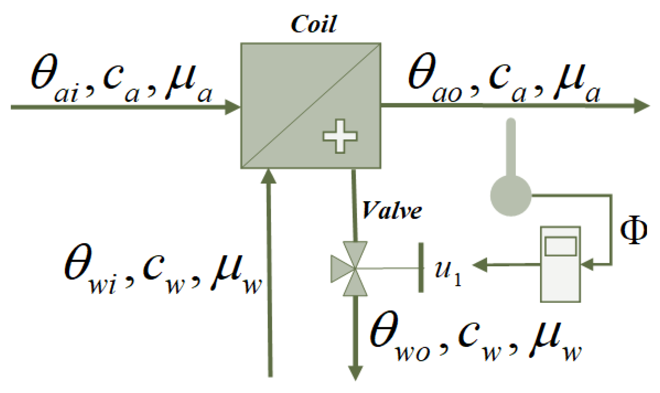
Figure 3.
Structure of control system.
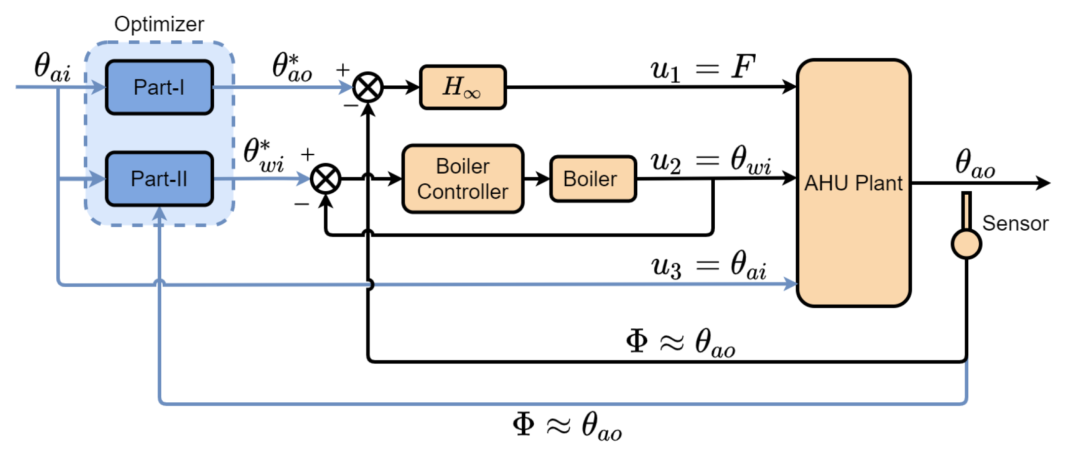
Figure 4.
Illustration of conventional control of .
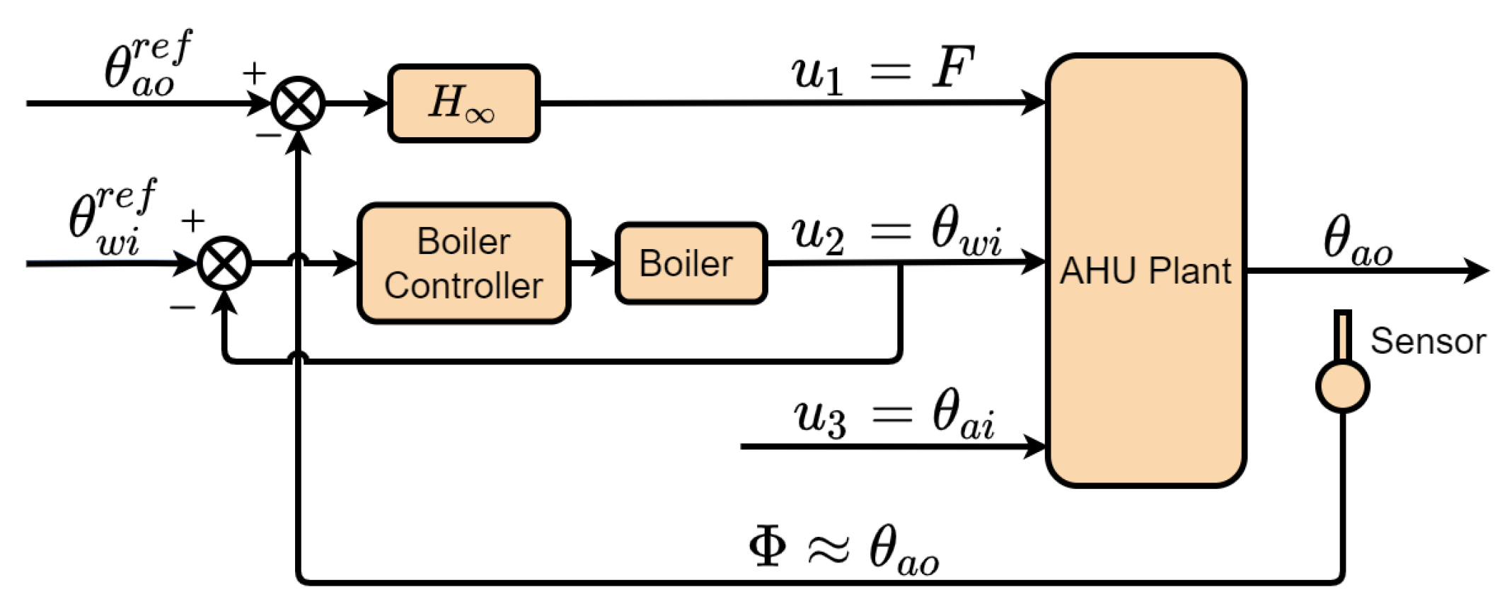
Figure 5.
AHU plant response with controller at three different thermal load conditions (square wave input).
Figure 5.
AHU plant response with controller at three different thermal load conditions (square wave input).

Figure 6.
AHU plant response with controller at three different thermal load conditions (step input).
Figure 6.
AHU plant response with controller at three different thermal load conditions (step input).

Figure 7.
AHU system power consumption with controller at three different thermal load conditions (square wave input).
Figure 7.
AHU system power consumption with controller at three different thermal load conditions (square wave input).
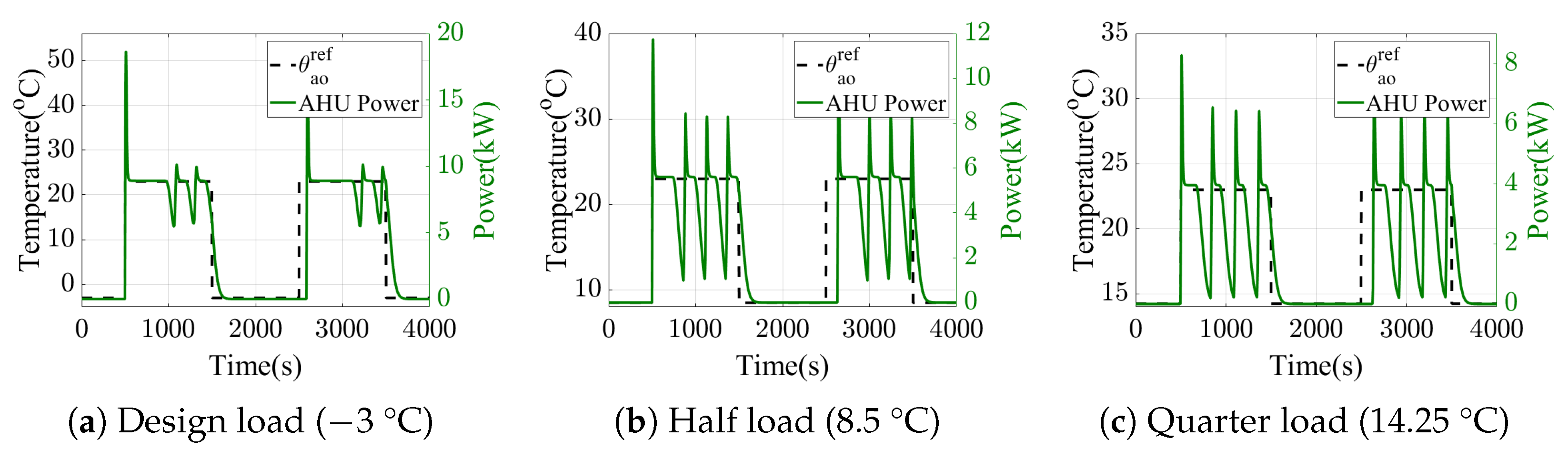
Figure 8.
AHU system power consumption with controller at three different thermal load conditions (step input).
Figure 8.
AHU system power consumption with controller at three different thermal load conditions (step input).
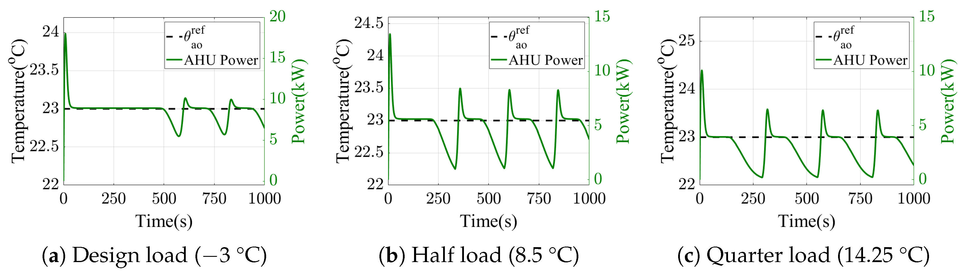
Figure 9.
Pareto optimal fronts generated at minimum (16 °C) and maximum (26 °C) outside temperatures recorded during summer.
Figure 9.
Pareto optimal fronts generated at minimum (16 °C) and maximum (26 °C) outside temperatures recorded during summer.

Figure 10.
Pareto optimal fronts generated at minimum ( °C) and maximum ( °C) outside temperatures recorded during winter.
Figure 10.
Pareto optimal fronts generated at minimum ( °C) and maximum ( °C) outside temperatures recorded during winter.

Figure 11.
System performance during typical warm day in Auckland (first day of January). (a) Optimized set-points. (b) Comfort level comparison. (c) AHU system power consumption for temperature control.
Figure 11.
System performance during typical warm day in Auckland (first day of January). (a) Optimized set-points. (b) Comfort level comparison. (c) AHU system power consumption for temperature control.

Figure 12.
System performance during typical cool day in Auckland (first day of June). (a) Optimized set points. (b) Comfort level comparison. (c) AHU system power consumption for temperature control.
Figure 12.
System performance during typical cool day in Auckland (first day of June). (a) Optimized set points. (b) Comfort level comparison. (c) AHU system power consumption for temperature control.


Table 1.
Search domain of decision variables.
| Decision Variable | Search Domain () | |
|---|---|---|
| (°C) | 19 | 25 |
| (°C) | 10 | 40 |
Table 2.
Overall energy performance of the AHU in kWh.
| Time Duration (t) | Energy Consumption (kWh) | Energy Saving (kWh) | |
|---|---|---|---|
| Without Optimizer () | With Optimizer () | ||
| First Day of January (24 h) | |||
| First Day of June (24 h) | |||
| Entire Year (8640 h) | |||
Table 3.
Number of time steps recorded with high comfort level values.
| Time Duration (N) | Number of Time Steps with Comfort Levels | Increase in Comfort Levels (%) | |
|---|---|---|---|
| Without Optimizer | With Optimizer | ||
| First Day of January (144 time steps) | 89 | 136 | |
| First Day of June (144 time steps) | 26 | 91 | |
| Entire Year (51,840 time steps) | |||
Disclaimer/Publisher’s Note: The statements, opinions and data contained in all publications are solely those of the individual author(s) and contributor(s) and not of MDPI and/or the editor(s). MDPI and/or the editor(s) disclaim responsibility for any injury to people or property resulting from any ideas, methods, instructions or products referred to in the content. |
© 2023 by the authors. Licensee MDPI, Basel, Switzerland. This article is an open access article distributed under the terms and conditions of the Creative Commons Attribution (CC BY) license (https://creativecommons.org/licenses/by/4.0/).
Share and Cite
MDPI and ACS Style
Wani, M.; Hafiz, F.; Swain, A.; Ukil, A. A Multi-Objective Approach to Robust Control of Air Handling Units for Optimized Energy Performance. Electronics 2023, 12, 661. https://doi.org/10.3390/electronics12030661
AMA Style
Wani M, Hafiz F, Swain A, Ukil A. A Multi-Objective Approach to Robust Control of Air Handling Units for Optimized Energy Performance. Electronics. 2023; 12(3):661. https://doi.org/10.3390/electronics12030661
Chicago/Turabian StyleWani, Mubashir, Faizal Hafiz, Akshya Swain, and Abhisek Ukil. 2023. "A Multi-Objective Approach to Robust Control of Air Handling Units for Optimized Energy Performance" Electronics 12, no. 3: 661. https://doi.org/10.3390/electronics12030661
Note that from the first issue of 2016, this journal uses article numbers instead of page numbers. See further details here.