Optimal Placement and Sizing of D-STATCOMs in Electrical Distribution Networks Using a Stochastic Mixed-Integer Convex Model

Abstract

This paper addresses the problem regarding the optimal placement and sizing of distribution static synchronous compensators (D-STATCOMs) in electrical distribution networks via a stochastic mixed-integer convex (SMIC) model in the complex domain. The proposed model employs a convexification technique based on the relaxation of hyperbolic constraints, transforming the nonlinear mixed-integer programming model into a convex one. The stochastic nature of renewable energy and demand is taken into account in multiple scenarios with three different levels of generation and demand. The proposed SMIC model adds the power transfer losses of the D-STATOMs in order to size them adequately. Two objectives are contemplated in the model with the aim of minimizing the annual installation and operating costs, which makes it multi-objective. Three simulation cases demonstrate the effectiveness of the stochastic convex model compared to three solvers in the General Algebraic Modeling System. The results show that the proposed model achieves a global optimum, reducing the annual operating costs by 29.25, 60.89, and 52.54% for the modified IEEE 33-, 69-, and 85-bus test systems, respectively.

1. Introduction

The efficient operation of electrical distribution grids has always been a challenge, which is becoming more relevant day by day with the constant growth in demand, taking these systems to their limits or deteriorating their operating state. Industrial loads have increased in recent years, more so than residential ones [1]. In addition, these loads are constantly growing, typically implying many rotating machines, which require large amounts of reactive power to maintain the balance of magnetic fields. These requirements degrade the power factor of electrical distribution systems, and they cause congestion in transmission lines, which limits the grid’s energy transfer capacity and causes low voltage issues [2,3,4].

Usually, utility companies install passive and active devices to enhance the operation of electrical distribution grids. These devices can be capacitor banks, distribution static synchronous compensators (D-STATCOMs), energy storage systems (batteries, supercapacitors, superconducting magnets, flywheels, among others), and distributed generators (coal-fired, solar, wind, and biomass power plants, among others) [5,6]. Capacitor banks have been proven to be a good solution for improving the operation of electrical distribution grids (enhancing voltage profiles and reducing power losses) because of their low cost. Nevertheless, they do not provide an optimal solution because they have a fixed capacity and cannot adequately compensate for the typical variations of an electrical distribution system [7], whereas D-STATCOMs work by regulating their output voltage via a self-turn-off power switching element to manage their reactive power. This mode of operation gives them an advantage over capacitor banks, as they can dynamically alleviate the distribution system’s reactive power requirements [8,9]. Therefore, it is necessary to properly locate and size D-STATCOMs to improve the load power factor and voltage profiles and increase the power transfer capacity of transmission lines in distribution systems at reasonable investment costs.

The problem regarding the optimal location, size, and operation of D-STATCOMs in electrical distribution grids has been studied in the specialized literature. In reference [10], a combination between a fuzzy multi-objective approach and the ant colony algorithm was proposed to optimize the simultaneous reconfiguration and allocation of photovoltaic (PV) generation and D-STATCOMs. This algorithm aimed to mitigate power losses and improve voltage profiles by considering the impact of both PV devices and D-STATCOMs. In reference [11], a heuristic technique using power loss and voltage indices was proposed to determine the optimal placement and sizing of D-STATCOMs in electrical distribution systems. This technique was evaluated through numerical validation on the IEEE 33-bus test system, albeit only under maximum load conditions. In reference [12], the authors proposed an approach that employs analytical and heuristic optimization techniques to identify the ideal location and size of D-STATCOMs. This work also outlined the typical objective functions used in this area of research, such as the indicators for voltage stability and power losses. Another study by [13] used a multi-objective particle swarm optimizer to determine the placement and size of D-STATCOMs while considering power grid reconfiguration. The objective functions were the minimization of active power losses, the voltage stability index, and the load capacity factor of distribution lines. However, this approach was limited, as it only considered the optimization process under maximum load conditions. This could lead to the oversizing of the compensating devices, given that active and reactive power consumption implies variable inputs. The authors of [14] used a discrete-continuous version of the vortex search algorithm to address the problem regarding the optimal location and size of D-STATCOMs in electric distribution networks. This algorithm had two stages; the first stage (the discrete part) selected the buses to install the D-STATCOMs, while the second stage (the continuous part) determined their optimal sizes. The authors of [15] combined the Chu and Beasley genetic algorithm (CBGA) and a second-order cone programming formulation to determine the optimal configuration (location and size) of D-STATCOMs in electric distribution networks. This combination could not ensure that the global optimum of the problem was found because of the random nature of the CBGA. Furthermore, the second-order cone formulation only minimized the total energy losses of each proposition of the CBGA, resulting in higher grid operating costs than those of the metaheuristic approach presented in [14].

Table 1. Summary of research works related to the siting and sizing of D-STATCOMs.

Methodology	Objective Function	Year	Ref.
Genetic algorithm	Minimization of power losses	2011	[16]
Artificial neural networks	Mitigation of voltage sags under faults	2012	[17]
Immune algorithm	Minimization of power losses and reduction of investment and operating costs	2014	[18]
Particle swarm optimization	Minimization of power losses and voltage profile improvement	2014	[19]
Ant colony optimization	Minimization of power losses and voltage profile improvement	2015	[10]
Sensitivity indices	Minimization of power losses and voltage profile improvement	2015	[20]
Harmony search algorithm	Minimization of power losses	2015	[21]
Heuristic search algorithm	Minimization of power losses	2016	[22]
Imperialist competitive algorithm	Minimization of energy costs and voltage profile improvement	2017	[23]
Discrete-continuous vortex search algorithm	Investment and operating costs reduction	2017	[15]
Modified crow search algorithm	Reducing line losses, maximizing economic benefits, improving voltage profiles, and reducing pollution levels	2018	[24]
Hybrid analytical-coyote	Minimization of active power losses and voltage profile improvement	2019	[25]
Modified sine-cosine algorithm	Minimization of power losses and voltage profile improvement	2020	[26]
GAMS software for the solution of the exact MINLP model	Reduction in investment and operating costs	2021	[27]

summarizes the proposed methodologies used to solve the optimal D-STATCOM location and sizing problem in electrical distribution grids.

Even though the works shown in Table 1 can yield outstanding results, none of them can guarantee the global optimum of the problem since the exact model addressed therein is a nonconvex, nonlinear mixed-integer programming one. The exact model was reformulated in [28,29]. These reformulations were based on a mixed-integer second-order cone model, which can ensure the global optimum using the branch-and-cut in combination with an interior-point method. However, these models neglect the stochastic part of generation and demand, which is caused by their uncertainties. Unlike these previous works, this study describes a stochastic mixed-integer convex model that considers three different load-generation conditions (i.e., low-, medium-, and high-generation and -demand levels) in order to locate and size D-STATOMs in an electrical distribution network under multiple operating conditions. Furthermore, the proposed model considers the power transfer losses generated by D-STATOMs through their voltage source converters, with the purpose of sizing these devices properly. This implies the following contributions:

i.

The description of a stochastic mixed-integer convex (SMIC) model for the optimal placement and sizing of D-STATCOMs in electrical distribution networks. The proposed SMIC model considers nine scenarios involving low-, medium-, and high-load-generation levels.

ii.

The addition of binary-polynomial constraints to the proposed SMIC model in order to model the power transfer losses of D-STATCOMs. These constraints are convexified using second-order cone relaxation.

iii.

The objective function of the proposed SMIC model is composed of two terms: minimizing the annual energy loss costs and the annualized investment costs related to installing a new D-STATCOM, which implies a multi-objective problem. A weight factor is used to solve the problem, as these terms are in conflict.

iv.

Three simulation cases are proposed to demonstrate the effectiveness of the stochastic convex model, and it is compared to three solvers available in the General Algebraic Modeling System (GAMS) software.

This study is organized as follows. Section 2 presents the exact formulation for the optimal placement and sizing of D-STATCOMs in electrical distribution networks. Section 3 relaxes the exact formulation into a convex model and presents the stochastic mixed-integer convex model. Section 4 describes the three test systems used, along with the load-generation scenarios. Section 5 shows the proposed SMIC model’s main results and analysis. Finally, the main conclusions are presented in Section 6.

2. Mathematical Model

The optimal location and sizing of D-STATCOMs in electrical distribution grids allow one to improve their operating conditions, which includes reducing line congestion and power losses and improving the voltage profiles. Therefore, not only is it essential to know where to locate these devices, but also what size should be used to avoid deteriorating the grid operating conditions. Therefore, a mathematical model is required to solve the D-STATCOM optimal location and sizing problem in electrical distribution networks. Because it has continuous and binary variables, this model is a nonlinear mixed-integer programming (MINLP) one. The continuous variables are associated with the voltages at the nodes, power injection at the nodes, and the power flowing through the transmission lines. On the other hand, the binary variables are related to the location of a D-STATCOM, i.e., in a particular node. The electrical distribution grid can be modeled as an oriented graph $\mathcal{G}=\left\{\mathcal{N},\mathcal{B}\right\}$, where $\mathcal{N}$ is the set of nodes and $\mathcal{B}\in \mathcal{N}\times \mathcal{N}$ is the set of branches [30]. Figure 1 illustrates an example of a generic branch l (or line) between node k and m, $l=\left(km\right)\in \mathcal{B}$. The nonlinear mixed-integer programming model for the problem under study is presented below:

2.1. Objective Function

The proposed objective function is composed of two parts, namely minimizing the yearly costs of energy losses ($f_1$) and reducing the annualized investment costs associated with installing a new D-STATCOM ($f_2$), as shown below:

$$\begin{array}{c}\hfill \begin{array}{cc}\hfill min& f=f_1+f_2\hfill \\ \hfill f_1& =\sigma T\sum _{l\in \mathcal{B}}\sum _{t\in \mathcal{T}}real\left\{\left(s_{lt}^s+s_{lt}^r\right)\right\}\Delta t\hfill \\ \hfill f_2& =\xi T\sum _{k\in \mathcal{N}}{h}_k\left(\alpha h_k^2+\beta h_k+\gamma \right)\hfill \end{array}\end{array}$$

(1)

where $\Delta t$ is a single time period of the analysis; $h_k$ is the optimal size for a D-STATCOM connected at node k; T denotes the time under analysis (generally one year); $\xi$ is a positive constant related to the annualized investment costs of installing a new D-STATCOM; and $\alpha$, $\beta$, and $\gamma$ are the cost coefficients of the cubic function employed to install a new D-STATCOM [29]. This cost function relates the operating voltage and the current apparent power rating of the D-STATCOM [31]. $s_{lt}^s$ and $s_{lt}^r$ represent the power flows of the line connected between nodes k and m, as shown in Figure 1. The superscript s denotes the power flow in the line from k to m, while the superscript r denotes the power flow in the line from m to k ($s_{lt}^s\ne s_{lt}^r$). $real\left(·\right)$ represents the real part of the complex number.

Remark 1. 

The proposed objective function (1) has two conflicting goals, which makes it difficult to solve the problem. This means that, while objective one ($f_1$) improves, objective two ($f_2$) becomes worse—and vice versa. Therefore, the proposed objective function is rewritten using a weight factor in order to allow the utility company to give higher priority to one objective, as shown below:

$$\begin{array}{c}\hfill f=\omega f_1+(1-\omega )f_2\end{array}$$

(2)

where $\omega \in [0,1]$ denotes the weight factor, which allows varying the weight of both objective functions.

Remark 2. 

The installation cost function (cubic function) of the D-STATCOM devices $f_2$ comes from the Siemens database, as described in [32,33]. This database presents the cost functions for flexible AC transmission system (FACTS) devices. All of their cost functions are in the form of a cubic function, and the differences between them are their coefficients.

2.2. Set of Constraints

The physical operations and regulation characteristics of electrical distribution grids give the set of constraints of this model. This set involves the apparent power balance at nodes, the power transmission capacity through the lines, the power limits of the generators, the maximum and minimum voltage levels, and the D-STATCOM size. The set of constraints is presented below:

2.2.1. Grid-Connected D-STATCOMs

The integration of a D-STATCOM is usually carried out through a voltage source converter (VSC). In general, in the optimal location and sizing problem of D-STATCOMs in electrical distribution grids, the power losses caused by VSCs are not modeled. This may lead to an error in the location or size optimal of a D-STATCOM. With this in mind, the VSC power losses are modeled as a quadratic function [34]:

$$\begin{array}{cc}\hfill s_{los{s}_{vsc}}=& b(c_0+c_1{s}_{st}+c_2{s}_{st}^2),\hfill \end{array}$$

(3)

where b is a binary variable that represents the operating state of the VSC ($b=1$ means that the VSC is operating, and $b=0$ means that it is not); $s_{st}$ denotes the apparent power flow between the D-STATCOM and the grid; $s_{los{s}_{vsc}}$ denotes the power losses in the VSC; $c_0$, $c_1$, and $c_2$ are coefficients that represent the different types of losses within a converter [35,36]; $c_0$ is the reference losses coefficient for no-load energizing, which is associated with the passive components of the VSC, such as the filter and transformer; and $c_1$ and $c_2$ are the switching and power conduction loss coefficients in the VSC, respectively [37].

On the other hand, the maximum size, location, and maximum number of D-STATCOMs are defined as

$$\begin{array}{cc}\hfill 0\le h_k\le z_k{s}_{st}^{max},& \forall k\in \mathcal{N}\hfill \end{array}$$

(4)

$$\begin{array}{cc}\hfill -h_k\le s_{st,kt}\le h_k,& \forall k\in \mathcal{N},\forall t\in \mathcal{T}\hfill \end{array}$$

(5)

$$\begin{array}{c}\hfill \sum _{k\in \mathcal{N}}{z}_k\le \eta ,\end{array}$$

(6)

$$\begin{array}{cc}\hfill z_k\in \left\{0,1\right\},& \forall k\in \mathcal{N},\hfill \end{array}$$

(7)

where $h_k$ is the auxiliary variable used to define the maximum values for the D-STATCOM; $s_{st,kt}$ is the apparent power of a D-STATCOM; $z_k$ is a binary variable that defines whether a D-STATCOM is connected at node k; and $\eta$ is the maximum number of D-STATCOMs available for installation. Finally, the relationship between the power of the D-STATCOM and the power delivered by the VSC to the grid is

$$\begin{array}{c}\hfill s_{st,kt}=s_{los{s}_{vsc}}+s_{vsc,kt},\end{array}$$

(8)

where $s_{vsc,kt}$ is the apparent power delivered by the VSC at node k.

2.2.2. Power Balance Equation

The power balance is given by the sum of generated and demand power at node k, which is equal to the injection power flow, as follows:

$$\begin{array}{cc}\hfill s_{kt}^g-s_{kt}^d+s_{vsc,kt}=\sum _{l\in L}\left(A_{kl}^{+}{s}_{lt}^s+A_{kl}^{-}{s}_{lt}^r\right),& \forall k\in \mathcal{N},\forall t\in \mathcal{T}\hfill \end{array}$$

(9)

where $s_{kt}^g$ and $s_{kt}^d$ are the generated and demanded power, respectively; $s_{vsc,kt}$ is the power injected by the VSC; $A^{+}$ contains the positive values of the node-to-branch incidence matrix A; and $A^{-}$ contains its negative values ($A=A^{+}+A^{-}$).

Remark 3. 

The subscript $kt$ denotes the element connected to node k at time t, and the subscript $lt$ represents the element connected to branch l at time t.

2.2.3. Power Flow Equation

The power flowing through a line and the maximum flow can be represented as

$$\begin{array}{c}\hfill s_{lt}^s=v_{kt}{y}_l^{*}{\left(v_{kt}-v_{mt}\right)}^{*},\forall l\in \mathcal{B},\forall t\in \mathcal{T}\end{array}$$

(10)

$$\begin{array}{c}\hfill s_{lt}^r=v_{mt}{y}_l^{*}{\left(v_{mt}-v_{kt}\right)}^{*},\forall l\in \mathcal{B},\forall t\in \mathcal{T}\end{array}$$

(11)

$$\begin{array}{c}\hfill ∥s_{lt}^s∥\le s_l^{max},\forall l\in \mathcal{B},\forall t\in \mathcal{T}\end{array}$$

(12)

$$\begin{array}{c}\hfill ∥s_{lt}^r∥\le s_l^{max},\forall l\in \mathcal{B},\forall t\in \mathcal{T}\end{array}$$

(13)

where $v_{kt}and{v}_{mt}$ is the complex voltage at node k (or m) at time t; $y_l$ is the admittance of branch l; ${(·)}^{*}$ denotes the conjugate of the complex number; and $s_l^{max}$ is the maximum power flow in branch l.

2.2.4. Operating Regulation

Regulatory policies bound voltage values for the satisfactory operation of electrical grids. The voltage at the slack node and the voltage limits are defined as

$$\begin{array}{cc}\hfill v_{0t}=v^{\mathrm{nom}}{e}^{j0},& \forall t\in \mathcal{T}\hfill \end{array}$$

(14)

$$\begin{array}{cc}\hfill v_{kt}\le v^{max},& \forall k\in \mathcal{N},\forall t\in \mathcal{T}\hfill \end{array}$$

(15)

$$\begin{array}{cc}\hfill v_{kt}\ge v^{min},& \forall k\in \mathcal{N},\forall t\in \mathcal{T}\hfill \end{array}$$

(16)

where $v_{0t}$ is the rated voltage at the substation (usually $v^{\mathrm{nom}}=1$ in per-unit), and $v^{max}$ and $v^{min}$ are the maximum and minimum voltages allowed in the grid.

2.3. Interpretation of the Mathematical Model

The mathematical model for the optimal D-STATCOM location and sizing problem in electrical distribution grids described from (1) to (16) contains continuous variables associated with the magnitudes and angles of the nodal voltages, as well as the active and reactive power injection of the generators and the D-STATCOMs. At the same time, this model includes the binary variables related to the location of the D-STATCOMs in the electrical network. Equations (1)–(16) of the MINLP have the following aspects. Expression (1) corresponds to the total costs for one year of operating the electrical distribution system, which is denoted by two terms: the first one, $f_1$, is associated with the annual costs of the energy losses, while the second one, $f_2$, is related to the yearly costs of installing a new D-STATCOM. Equation (3) represents the power losses of a VSC, which are given by passive components, the switching function, and energy transfer. Inequalities (4) and (5) define the maximum and minimum limits of the D-STATCOMs installed in the electrical network, while inequality (6) limits the maximum number of D-STATCOMs to be installed. Equation (8) represents the reactive power flow between the D-STATCOMs and the grid. Expression (9) is the apparent power balance for each node and period. Equations (10) and (11) represent the power flowing through the transmission lines for each branch and period. In contrast, inequalities (12) and (13) denote their maximum power flow. Finally, inequalities (15) and (16) are the upper and lower voltage bounds of each node and period, respectively.

3. Convex Reformulation

The above-presented mixed-integer nonlinear model for the problem under study is difficult to solve since it falls into the NP-hard category. Therefore, metaheuristic methods are typically used to solve it in the literature. However, none of these methods can ensure a global optimum, and many of them require tuning several parameters, thus affecting their performance. Unlike these methods, this study transforms the model into a convex one through relaxation. The main advantage of this convex model is that the global optimum is guaranteed and does not require parameter adjustment.

3.1. Approximation to a Linear Function for D-STATCOM Costs

$f_2$ is a non-convex and cubic function. Therefore, the global optimum of the problem cannot be guaranteed. However, it is possible to make a linear approximation of this function, as the size range ($<2$ MVAr) of the D-STATCOMs considered in this paper allows it. Performing a Taylor’s expansion around $h_k=0$ yields the following expression:

$$\begin{array}{c}\hfill f_2=T\xi \sum _{k\in N}\gamma h_k.\end{array}$$

(17)

3.2. Conic Representation of the Power Flow Equations

The power flow equations shown in (10) and (11) are nonconvex because they are equalities and there are products between voltages. Two auxiliary variables are generated to transform the model into a standard second-order cone approximation [38]. The auxiliary variables are defined as

$$\begin{array}{c}\hfill u_{kt}=v_{kt}{v}_{kt}^{*}={∥v_{kt}∥}^2,\end{array}$$

(18)

$$\begin{array}{c}\hfill w_{lt}=v_{kt}{v}_{mt}^{*}\end{array}$$

(19)

where $u_{kt}\in \mathcal{R}$ is the voltage squared at the node k, and $w_{lt}\in \mathcal{C}$ is the product of the voltages in branch l.

Now, these auxiliary variables (18) and (19) are replaced into (10) and (11), yielding

$$\begin{array}{c}\hfill s_{lt}^s=y_l^{*}\left(u_{kt}-w_{lt}\right),\end{array}$$

(20)

$$\begin{array}{c}\hfill s_{lt}^r=y_l^{*}\left(u_{mt}-w_{lt}^{*}\right).\end{array}$$

(21)

Observe that the new power flow equations, (20) and (21), depend on the auxiliary variables, as shown below:

$$\begin{array}{c}\hfill \begin{array}{cc}\hfill w_{lt}& =v_{kt}{v}_{mt}^{*}\hfill \\ \hfill w_{lt}{w}_{kmt}^{*}& =v_{kt}{v}_{mt}^{*}{v}_{mt}{v}_{kt}^{*}\hfill \\ \hfill {∥w_{lt}∥}^2& ={∥v_{kt}∥}^2{∥v_{mt}∥}^2\hfill \\ \hfill {∥w_{lt}∥}^2& =u_{kt}{u}_{mt}\hfill \end{array}\end{array}$$

(22)

Here, the nonconvex form has remained, so it is necessary to rewrite it as a hyperbolic constraint,

$$\begin{array}{c}\hfill \begin{array}{cc}\hfill {∥w_{lt}∥}^2& =u_{kt}{u}_{mt}\hfill \\ \hfill {∥w_{lt}∥}^2& =\frac{1}{4}{\left(u_{kt}+u_{mt}\right)}^2-\frac{1}{4}{\left(u_{kt}-u_{mt}\right)}^2\hfill \\ \hfill {\left(u_{kt}-u_{mt}\right)}^2+{∥2w_{lt}∥}^2& ={\left(u_{kt}+u_{mt}\right)}^2\hfill \\ \hfill ∥\begin{array}{c}2w_{lt}\\ u_{kt}-u_{mt}\end{array}∥& =u_{kt}+u_{mt}.\hfill \end{array}\end{array}$$

(23)

Note that the hyperbolic constraint (23) continues to maintain its nonconvex form. Thereupon, this expression is relaxed in order to convert it into the convex constraint of a second-order cone, as follows:

$$\begin{array}{cc}\hfill ∥\begin{array}{c}2w_{lt}\\ u_{kt}-u_{mt}\end{array}∥& \le u_{kt}+u_{mt}.\hfill \end{array}$$

(24)

3.3. Conic Representation of VSC Power Losses

The VSC power losses expressed in (3) are a nonlinear nonconvex equation that complicates the problem’s solution. Hence, this equation is also transformed into a linear constraint, as follows:

$$\begin{array}{cc}\hfill s_{los{s}_{vsc},kt}=& b_{kt}{c}_0+c_1{s}_{abs,kt}^{abs}+c_2{k}_{kt},\hfill \end{array}$$

(25)

with

$$\begin{array}{cc}\hfill s_{abs,kt}& =|s_{st,kt}|,\hfill \end{array}$$

(26)

$$\begin{array}{cc}\hfill k_{kt}=s_{st,kt}^2& =q_{st,kt}^2..\hfill \end{array}$$

(27)

The constraint (26) can be rewritten as a linear constraint:

$$\begin{array}{c}\hfill -s_{st,kt}\le s_{abs,kt}\le s_{st,kt}.\end{array}$$

(28)

The quadratic constraint (27) can be converted into a second-order cone constraint, as follows:

$$\begin{array}{c}\hfill \begin{array}{cc}\hfill k_{kt}=& q_{st,kt}^2\hfill \\ \hfill {\displaystyle \frac{1}{4}}{(k_{kt}+1)}^2-{\displaystyle \frac{1}{4}}{(k_{kt}-1)}^2=& {∥q_{st,kt}∥}^2\hfill \\ \hfill {(k_{kt}+1)}^2=& {∥2q_{st,kt}∥}^2+{(k_{kt}-1)}^2\hfill \\ \hfill ∥\begin{array}{c}2q_{st,kt}\\ 1-k_{kt}\end{array}∥=& k_{kt}+1\hfill \\ \hfill ∥\begin{array}{c}2q_{st,kt}\\ 1-k_{kt}\end{array}∥\le & k_{kt}+1.\hfill \end{array}\end{array}$$

(29)

3.4. Proposed Mixed-Integer Convex Model

Using the above transformations, the exact model for the optimal D-STATCOM location and sizing problem in electrical distribution grids ((1)–(16)) is transformed into a multi-objective mixed-integer convex model:

$$\min f=\omega f_1+(1-\omega )f_2$$

(30)

$$\begin{array}{cc}\hfill & f_1=\sigma T\sum _{l\in \mathcal{B}}\sum _{t\in \mathcal{T}}real\left\{\left(s_{lt}^s+s_{lt}^r\right)\right\}\Delta t\hfill \end{array}$$

(31)

$$\begin{array}{cc}\hfill & f_2=T\xi \sum _{k\in \mathcal{N}}\gamma h_k\hfill \end{array}$$

(32)

$$\begin{array}{cc}\hfill & s_{kt}^g-s_{kt}^d+s_{vsc,kt}=\sum _{l\in \mathcal{B}}\left(A_{kl}^{+}{s}_{lt}^s+A_{kl}^{-}{s}_{lt}^r\right),\forall k\in \mathcal{N},\forall t\in \mathcal{T}\hfill \end{array}$$

(33)

$$\begin{array}{cc}\hfill & s_{lt}^s=y_l^{*}\left(u_{kt}-w_{lt}\right),\forall l\in \mathcal{B},\forall t\in \mathcal{T}\hfill \end{array}$$

(34)

$$\begin{array}{cc}\hfill & s_{lt}^r=y_l^{*}\left(u_{mt}-w_{lt}^{*}\right),\forall l\in \mathcal{B},\forall t\in \mathcal{T}\hfill \end{array}$$

(35)

$$\begin{array}{cc}\hfill & ∥s_{lt}^s∥\le s_l^{max},\forall l\in \mathcal{B},\forall t\in \mathcal{T}\hfill \end{array}$$

(36)

$$\begin{array}{cc}\hfill & ∥s_{lt}^r∥\le s_l^{max},\forall l\in \mathcal{B},\forall t\in \mathcal{T}\hfill \end{array}$$

(37)

$$\begin{array}{cc}\hfill & u_{0t}={\left(v^{\mathrm{nom}}\right)}^2,\forall t\in \mathcal{T}\hfill \end{array}$$

(38)

$$\begin{array}{cc}\hfill & ∥\begin{array}{c}2w_{lt}\\ u_{kt}-u_{mt}\end{array}∥\le u_{kt}+u_{mt},\forall k\in \mathcal{N},\forall t\in \mathcal{T}\hfill \end{array}$$

(39)

$$\begin{array}{cc}\hfill & u^{min}\le u_{kt}\le u^{max},\forall k\in \mathcal{N},\forall t\in \mathcal{T}\hfill \end{array}$$

(40)

$$\begin{array}{cc}\hfill & -s_{st,kt}\le s_{abs,kt}\le s_{st,kt},\forall k\in \mathcal{N},\forall t\in \mathcal{T}\hfill \end{array}$$

(41)

$$\begin{array}{cc}\hfill & s_{st,kt}=s_{los{s}_{vsc}}+s_{vsc,kt},\forall k\in \mathcal{N},\forall t\in \mathcal{T}\hfill \end{array}$$

(42)

$$\begin{array}{cc}\hfill & -s_{st,kt}\le s_{abs,kt}\le s_{st,kt},\forall k\in \mathcal{N},\forall t\in \mathcal{T}\hfill \end{array}$$

(43)

$$\begin{array}{cc}\hfill & s_{los{s}_{vsc},kt}=b_{kt}{c}_0+c_1{s}_{abs,kt}+c_2{k}_{kt},\forall k\in \mathcal{N},\forall t\in \mathcal{T}\hfill \end{array}$$

(44)

$$\begin{array}{cc}\hfill & ∥\begin{array}{c}2q_{st,kt}\\ 1-k_{kt}\end{array}∥\le k_{kt}+1,\forall k\in \mathcal{N},\forall t\in \mathcal{T}\hfill \end{array}$$

(45)

$$\begin{array}{cc}\hfill & 0\le h_k\le z_k{s}_{st}^{max},\forall k\in \mathcal{N}\hfill \end{array}$$

(46)

$$\begin{array}{cc}\hfill & -h_k\le s_{st,kt}\le h_k,\forall k\in \mathcal{N},\forall t\in \mathcal{T}\hfill \end{array}$$

(47)

$$\begin{array}{cc}\hfill & \sum _{k\in \mathcal{N}}{z}_k\le \eta \hfill \end{array}$$

(48)

$$\begin{array}{cc}\hfill & z_k\in \left\{0,1\right\},\forall k\in \mathcal{N}\hfill \end{array}$$

(49)

with $u^{\min }={\left(v^{\min }\right)}^2$ and $u^{\max }={\left(v^{\max }\right)}^2$. This model allows finding the global optimum of the nonconvex problem if the second-order cone constraints are well-defined conditions, as proven in [39].

The convex mathematical model for the optimal location and sizing of the D-STATCOM devices in electrical distribution networks formulated from (30) to (49) presents continuous variables associated with the squared magnitudes of the nodal voltages, as well as the active and reactive power injections of the generators and the D-STATCOMs. At the same time, this model includes the binary variables related to the location of the D-STATCOMs in the electrical network. Equations (30)–(49) of the convex mathematical model have the following aspects. Equation (30) is the total costs for one year of operating an electrical distribution system, which is represented by two terms: the first one (31), $f_1$, remains the annual costs of the energy losses. While the second one (32), $f_2$, is the yearly costs of installing a new D-STATCOM in linearized form to be convex. Expression (33) is the apparent power balance for each node and period. Expressions (34) and (35) are the power flowing through the transmission lines for each branch and period in function of the auxiliary variables $u_{kt}$ and $w_{lt}$, respectively, and inequalities (36) and (37) are their maximum power flow represented as a conical constraint shape. Equation (38) denotes the nominal voltage at the substation (usually 1 in per-unit). Inequality (39) is a second-order cone constraint for the auxiliary variables. Inequality (40) represents the regulation bound of the voltage squared at each node. Inequality (41) is the maximum apparent power flowing through the VSC. Equation (42) is apparently power injected (or absorbed) by the D-STATCOM, while inequality (43) represents its maximum power flow. Equation (44) is the power loss in the VSC in function of the auxiliary variables $s_{abs,kt}$ and $k_{kt}$. Expression (45) is the second-order cone constraints that correspond to the power losses by VSCs. Inequalities (46) and (47) represent the maximum and minimum limits of the D-STATCOMs installed in the electrical network, while inequality (48) limits the maximum number of D-STATCOMs to be installed, and Equation (49) represents the binary variable that defines whether a D-STATCOM is connected at node k.

3.5. Stochastic Mixed-Integer Convex Model

An electrical distribution system can have many operating states, as the generation from renewable sources and the demand are constantly changing. Therefore, for the problem under study, it is necessary to define a minimum number of possible scenarios. In this sense, the expected value of the objective function (30) can be formulated as a sample average approximation [40], which is defined as:

$$\begin{array}{cc}\hfill minE(f_1,f_2,{\zeta }_n)& =\sum _{n\in \mathcal{E}}{\zeta }_{n}f,\hfill \end{array}$$

(50)

where ${\zeta }_n$ is the probability of some scenario occurring and $\mathcal{E}$ is the set of scenarios.

Remark 4. 

Note that the objective function (50) continues to be affine. Therefore, it is convex, and the global optimum of the problem can be ensured. However, the number of scenarios must be finite in order for the problem to be tractable.

Finally, the proposed stochastic mixed-integer convex (SMIC) model takes the following form:

$$\begin{array}{c}\hfill \begin{array}{cc}\hfill min& \sum _{n\in \mathcal{E}}{\zeta }_{n}f\hfill \\ \hfill \mathrm{subject}\mathrm{to}& \left(31\right)-\left(49\right).\hfill \end{array}\end{array}$$

(51)

4. Test System

Numerical experiments were performed to validate the proposed SMIC model on three modified distribution systems, namely the IEEE 33-, 69-, and 85-bus test systems. All of the systems have three PV solar generators, and their main characteristics are described below:

4.1. Modified IEEE 33-Bus Test System

The IEEE 33-bus test system features a radial topology consisting of 33 buses and 32 lines. This system operates at 12.66 kV and experiences a peak demand of $3715+j2300$ kVA, resulting in power losses of $210.9876$ kW and $143.1283$ kvar at peak load. This study added three PV solar generators with rated powers of 801.8 kW, 1091.3 kW, and 1053.6 kW to buses 13, 24, and 30, respectively. The locations and sizes of these generators were determined based on previous works [41]. The modified IEEE 33-bus test system’s topology is depicted in Figure 2a, with voltage and power base values of 12.66 kV and 1 MW, respectively. The data regarding peak consumptions and transmission lines used for this test system can be found in [42].

4.2. Modified IEEE 69-Bus Test System

The IEEE 69-bus test system comprises 69 buses and 68 lines with a radial topology. This system operates at 12.66 kV and has a peak demand of $3890.7+j2693.6$ kVA, which generates, in peak hours, power losses of $224.9520$ kW and $102.3559$ kvar, respectively. The modification includes three PV solar generators at nodes 11, 18, and 61, with rated powers of 1631.31 kW, 463.33 kW, and 503.80 kW, respectively. The location and size of the PV solar generators were taken from [41]. The topology of the modified IEEE 69-bus test system is illustrated in Figure 2b, and its base values for voltage and power are 12.66 kV and 1 MW, respectively. This test system’s data, namely the peak consumptions and transmission lines, can be consulted in [42].

4.3. Modified IEEE 85-Bus Test System

The IEEE 85-bus test system is fitted with 85 buses and 84 lines arranged in a radial topology, and it operates at 11 kV with a peak demand of $2570.28+j2622.20$ kVA. This test system’s data, namely its peak consumptions and transmission lines, can be consulted in [43]. Additionally, three PV solar generators were added to buses 35, 67, and 71, with rated powers of 526.8 kW, 380.1 kW, and 1719 kW, respectively. The location and size of these generators were also taken from [43]. The modified IEEE 69-bus test system, with a base voltage of 12.66 kV and a base power of 1 MW, is shown in Figure 2c.

4.4. Load-Generation Scenario

When it comes to analyzing stochastic scenarios, numbers are vital; achieving an accurate and tractable model requires an appropriate number of scenarios. This study considers three different generation and demand conditions (corresponding to low-, medium-, and high-generation and demand levels). These scenarios generate nine possible combinations of generation and demand, each with a corresponding probability. While increasing the number of scenarios might improve the model’s accuracy, the additional computational effort required does not sufficiently justify the benefit.

Table 2. Probability of load-generation scenarios.

Scenario	Load-Generation	Probability (${\mathit{\zeta }}_{\mathit{n}}$)
1	Low/low	0.2210
2	Low/medium	0.0443
3	Low/high	0.0676
4	Medium/low	0.2767
5	Medium/medium	0.0554
6	Medium/high	0.0845
7	High/low	0.0845
8	High/medium	0.0332
9	High/high	0.0507

shows the probability of each scenario considered in this study.

Table 3. Parameter data to calculate the annual investment costs of D-STATCOMs.

Par.	Value	Unit	Par.	Value	Unit
$\sigma$	0.1390	USD/kWh	T	365	Days
${\Delta }_h$	0.50	h	$\alpha$	0.30	USD/MVAr${}^3$
$\beta$	−305.10	USD/MVAr${}^2$	$\gamma$	127,380	USD/MVAr
$k_1$	6/2190	1/Days	$k_2$	10	Years

presents the parameter data taken from [29] for this study.

5. Numerical Implementation

The numerical implementation of the proposed SMIC model was conducted in MATLAB $2021b$, using the CVX [44] and GUROBI solvers [45]. Computation was carried out on a 64-bit version of Microsoft Windows 10 on a personal computer with an Intel Quad-Core i7-7700HQ processor and 16.0 GB RAM. To assess the effectiveness of the proposed model, the exact MINLP model was solved using the BONMIN, CONOPT, and GUROBI solvers in GAMS.

Three simulation cases were analyzed:

C1:

The proposed model was compared with GAMS, only considering the installation of three D-STATCOMs.

C2:

The impact on the total annual operating costs of the number of D-STATCOMs available for installation was assessed by varying the number of devices from 0 to 5.

C3:

The Pareto front was formed by analyzing the trade-off between the costs of the D-STATCOMs and the annual energy loss costs, which are conflicting objectives.

5.1. Analysis of Case 1 (C1)

This scenario assesses the performance of the proposed SMIC model, solved using CVX and GUROBI, compared to GAMS with three different available solvers. The results of each component of the objective function regarding the three electrical distribution test systems are shown in

Table 4. Optimal location and size reached by the proposed SMIC model and the GAMS solvers.

			${\mathit{f}}^{\mathbf{annual}}$	${\mathit{f}}^{\mathbf{loss}}$	${\mathit{f}}^{\mathbf{invest}}$
Method	Location (Bus)	Size (k)	(USD/year)	(USD/year)	(USD/year)
	IEEE 33-bus test system
Ben. case			65,324.25	65,324.25	0.00
CONOPT	$\{30,32,33\}$	$\{538.55,113.67,28.38\}$	48,464.31	39,803.98	8660.33
BONMIN	$\{14,30,32\}$	$\{197.49,453.29,142.53\}$	46,212.30	36,115.04	10,097.26
GUROBI	$\{13,30,32\}$	$\{202.96,451.01,142.54\}$	46,243.04	36,105.07	10,137.98
SMIC	$\{14,30,32\}$	$\{197.49,453.29,142.53\}$	46,212.30	36,115.04	10,097.26
	IEEE 69-bus test system
Ben. case			112,740.90	112,740.90	0.00
CONOPT	$\{63,64,65\}$	$\{572.64,120.30,31.16\}$	45,329.51	39,803.98	9223.70
GUROBI	$\{21,61,64\}$	$\{109.99,578.90,153.25\}$	44,082.85	33,810.49	10,272.36
SMIC	$\{21,61,64\}$	$\{109.99,578.90,153.25\}$	44,082.85	33,810.49	10,272.36
	IEEE 89-bus test system
Ben. case			102,369.39	102,369.39	0.00
CONOPT	$\{27,52,68\}$	$\{439.58,328.83,431.30\}$	49,062.63	33,795.46	15,267.17
BONMIN	$\{38,52,73\}$	$\{331.48,381.82,399.55\}$	51,045.58	36,882.55	14,163.03
GUROBI	$\{65,70,75\}$	$\{586.54,134.11,118.05\}$	66,816.56	56,144.56	10,672.00
SMIC	$\{12,34,67\}$	$\{247.46,536.40,452.22\}$	48,581.90	32,853.47	15,728.43

.

From Table 4, it is possible to state that:

• The proposed SMIC model for the three test systems finds the best solutions (global optima) with objective function values of USD 46,212.30, USD 44,082.85, and USD 48,581.90. These solutions were obtained from the exact costs function (1). Comparing the benchmark cases to the best solutions revealed significant reductions of 29.25%, 60.89%, and 52.54% for the modified IEEE 33-, 69-, and 85-bus test systems, respectively.
• For the modified IEEE 33-bus test system, it can be noted that the BONMIN solver reached the same solution as the proposed SMIC model. In contrast, the CONOPT and GUROBI solvers achieved the worst solutions (local optima), reducing the annual operating costs by 25.81% and 29.21%, respectively.
• As for the modified IEEE 69-bus test system, the BONMIN solver did not yield any feasible solution due to convergence issues. On the other hand, the GUROBI solver found the same solution as the proposed SMIC model, and the CONOPT solver reached a local optimum, reducing the annual operating cost by 59.79%.
• For the modified IEEE 85-bus test system, it is evident that none of the solvers could attain the global optimum of the problem, and only local optima were found. In this case, the CONOPT solver reported a better solution than other solvers, which indicates that none of the solvers outperformed the other.

Figure 3 compares the voltage profiles of the test systems, considering the D-STATCOMs installed (or not).

From the voltage profiles shown in Figure 3, it is possible to state that, when the D-STATCOMs are included in the test systems, the voltage profiles are improved, remaining closer to their reference values ($\approx 1pu$). Note that, in Figure 3a, the worst voltage profile when the D-STATCOMs are installed is 0.9890 pu at node 8—whereas without D-STATCOMs, the worst voltage profile is 0.9677 pu at node 18, improving the voltage profile by 2.2%. For the 69-bus test system, the worst voltage profiles (see Figure 3b) with and without D-STATCOMs are 0.9942 pu at node 50 and 0.9789 pu at node 65, respectively. For this test system, the voltage profile is enhanced by 1.5%. In the case of the 69-bus test system, the worst voltage profiles with and without D-STATCOMs are 0.9804 pu and 0.9477 pu, both at node 84. The voltage profile is thus improved by 3.4%.

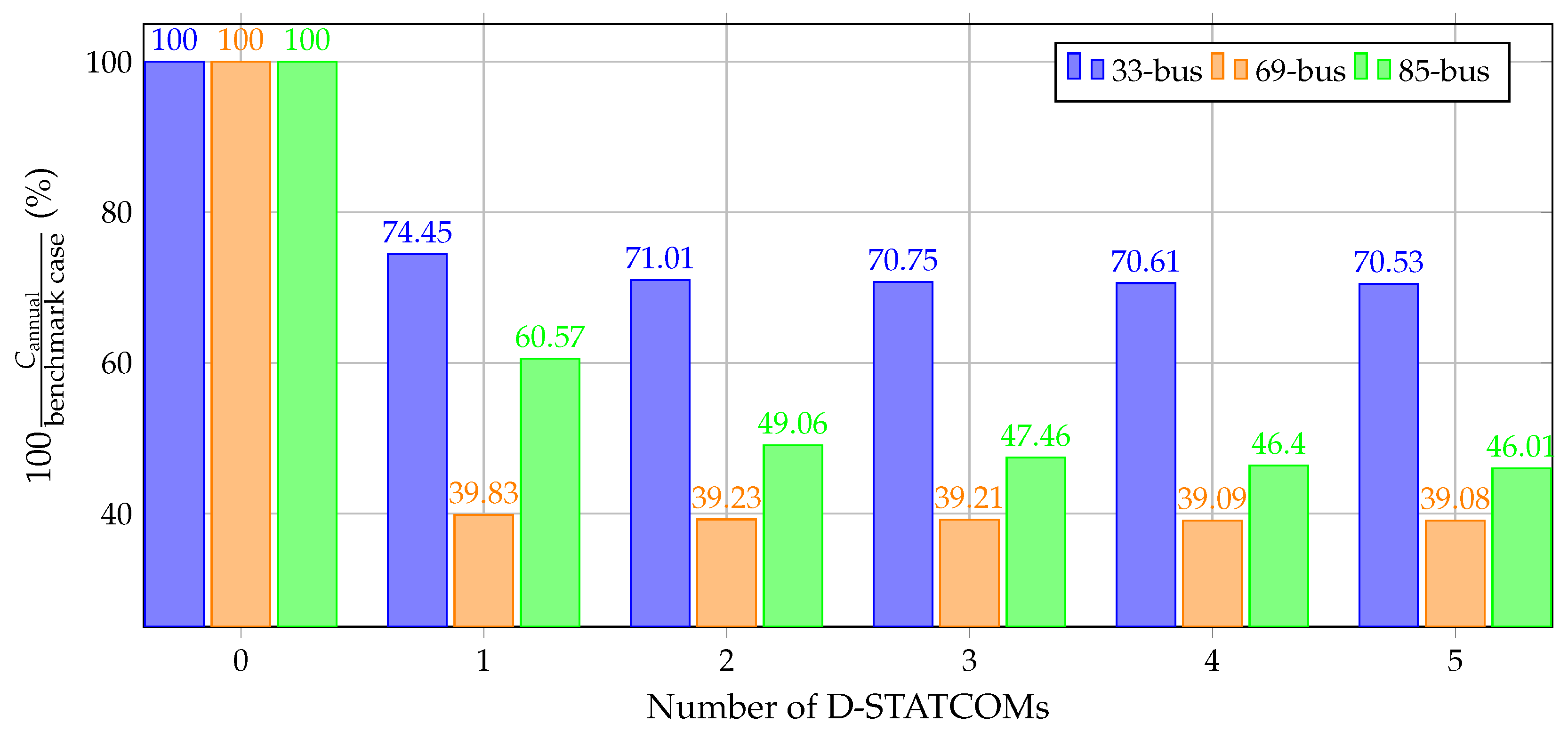
5.2. Analysis of Case 2 (C2)

This scenario analyzes the impact of varying the number of D-STATCOMS installed on the annual operating costs. The availability of D-STATCOMS to be installed goes from 1 to 5. This is depicted in Figure 4.

Figure 4 shows that, after installing the third D-STATCOM, the objective functions do not improve considerably. This indicates that installing more D-STATCOMs would not significantly reduce the annual operating costs of electrical networks. It can also be noted that the cost reduction is imperceptible between three and five D-STATCOMs installed. In these intervals, the annual operating costs are only reduced by 0.22%, 0.13%, and 1.45% for the modified IEEE 33-, 69-, and 85-bus test systems, respectively. For the first two test systems, it is not worth installing more than three D-STATCOMs, since the respective reductions in dollars per year of operation are USD 143.71 and USD 146.56. In contrast, the modified IEEE 85-bus test system shows a reduction of USD 1484.35 per year of operation. Hence, the decision to install more than three depends on the utility company.

5.3. Analysis of Case 3 (C3)

This section shows the Pareto set by varying the weight factor ($\omega$) of the multi-objective function (2) from 0 to 1 in steps of 0.1.

Table 5. Pareto set attained with the weight factor methodology.

Factor ($\mathit{\omega }$)	${\mathit{C}}_{\mathbf{annual}}$ (USD/year)	${\mathit{C}}_{\mathbf{loss}}$ (USD/year)	${\mathit{C}}_{\mathbf{invest}}$ (USD/year)
	IEEE 33-bus test system
0.0	65,324.25	65,324.25	0
0.1	65,324.25	65,324.25	0
0.2	47,707.61	37,002.80	9005.45
0.3	46,341.15	36,390.38	9950.77
0.4	46,276.73	36,252.71	10,024.01
0.5	46,212.31	36,115.05	10,097.26
0.6	46,379.65	36,172.90	10,206.75
0.7	46,395.17	36,172.01	10,223.16
0.8	46,410.70	36,171.13	10,239.57
0.9	46,412.49	36,272.77	10,339.72
1.0	104,613.34	32,121.99	72,491.35
	IEEE 69-bus test system
0.0	112,740.90	112,740.90	0
0.1	112,740.90	112,740.90	0
0.2	44,757.04	35,202.5	9554.54
0.3	44,754.02	34,336.33	10,417.69
0.4	46,332.37	33,331.98	13,000.39
0.5	44,082.85	33,810.49	10,272.36
0.6	44,101.20	33,577.67	10,523.53
0.7	44,119.56	33,344.86	10,774.70
0.8	44,230.72	33,501.36	10,729.36
0.9	48,705.06	30,205.07	18,499.99
1.0	50,821.03	30,109.31	20,711.72
	IEEE 85-bus test system
0.0	102,369.39	102,369.39	0
0.1	102,369.39	102,369.39	0
0.2	90,641.97	88,022.15	2619.82
0.3	56,682.66	47,597.36	9085.30
0.4	51,604.91	39,705.79	11,899.12
0.5	48,581.90	32,853.47	15,728.43
0.6	49,777.82	32,370.34	17,407.48
0.7	49,701.84	28,554.90	21,146.94
0.8	52,111.75	28,893.70	23,218.05
0.9	52,287.42	28,302.63	23,984.79
1.0	66,766.11	27,425.10	39,341.01

lists the objective function values for three test systems, which are computed using the SMIC model.

The results from the Pareto front in Table 5 reveal the following insights:

• There is a trade-off between the annual costs of energy losses and those associated with investment costs in D-STATCOMs, as improving one objective leads to the deterioration of the other and vice versa. Specifically, the two extreme solutions are characterized by: (i) annual energy losses costs of USD $65,324.25$, USD $112,740.90$, and USD $10,2369.39$ per year for the modified IEEE 33-, 69-, and 85-bus test systems, respectively, with zero investments (i.e., $\omega =0$); and (ii) increased investments of USD $72,491.35$, USD $20,711.72$, and USD $39,341.01$ per year of operation (i.e., $\omega =1$), which results in the lowest cost of energy losses for the three test systems.
• The optimal solution for each test system in Table 4 is achieved via the proposed SMIC model, which corresponds to the minimum cost reported in the multi-objective case (i.e., when $\omega =0.5$). This indicates that the scaling factor of the objective function for the single-objective case does not significantly affect the final result of the convex model. However, the main advantage of having a Pareto front is that it offers a range of possibilities in order for a utility company to choose the most suitable option based on its investment capabilities.

6. Conclusions and Future Works

This study addressed the optimal placement and sizing of D-STATCOMs in electrical distribution networks by introducing a SMIC model in the complex domain. The proposed model employed a convexification technique based on hyperbolic constraint relaxation, which transformed the MINLP model into a convex one. The stochastic nature of renewable energy and demand was accounted for through multiple scenarios, representing different levels of generation and demand. The effectiveness of the proposed model was evaluated for three test systems and compared to three GAMS software solvers. The results showed that the proposed model achieved the global optimum, reducing the annual operating costs by 29.25%, 60.89%, and 52.54% for the modified IEEE 33-, 69-, and 85-bus test systems, respectively. In some cases, the GAMS software solvers also reached the global optimum, but in other cases, they failed to converge and often got stuck in local optima. Overall, the proposed SMIC model demonstrated significant improvements over existing methods.

The effect of varying the number of available D-STATCOMs (from 0 to 5) on the annual operating costs was also analyzed in this work, which showed that, after three D-STATCOMs, the improvement in the objective function was imperceptible. This was supported by analyzing the differences regarding the annual energy losses cost reductions associated with installing three D-STATCOMs and allocating five. These reductions were USD 143.71, USD 146.56, and USD 1484.35 for the modified IEEE 33-, 69-, and 85-bus test systems, which are not significant values.

Analyzing the formulation of the problem revealed a conflict between the two objective functions. However, the weight factor-based multi-objective approach provided several feasible options for the utility operator to implement based on its investment capabilities. Additionally, the study found that $\omega =0.50$ represents the global minimum for the single-objective function approach, thus confirming the effectiveness of the proposed SMIC model in finding the global optimum during each evaluation.

As future works, the following investigation topics can be analyzed: (i) the joint optimization of the placement and sizing of renewable energy resources and D-STATCOMs in order to enhance grid performance within a specific planning horizon while considering annual load increase; and (ii) the implementation of the proposed SMIC model in other problems related to electrical distribution networks.

References

- Jardini, J.; Tahan, C.; Gouvea, M.; Ahn, S.; Figueiredo, F. Daily load profiles for residential, commercial and industrial low voltage consumers. IEEE Trans. Power Deliv. 2000, 15, 375–380. [Google Scholar] [CrossRef] [Green Version]
- Rahimzadeh, S.; Bina, M.T. Looking for optimal number and placement of FACTS devices to manage the transmission congestion. Energy Convers. Manag. 2011, 52, 437–446. [Google Scholar] [CrossRef]
- Tuzikova, V.; Tlusty, J.; Muller, Z. A novel power losses reduction method based on a particle swarm optimization algorithm using STATCOM. Energies 2018, 11, 2851. [Google Scholar] [CrossRef] [Green Version]
- Abba, S.; Najashi, B.G.; Rotimi, A.; Musa, B.; Yimen, N.; Kawu, S.; Lawan, S.; Dagbasi, M. Emerging Harris Hawks Optimization based load demand forecasting and optimal sizing of stand-alone hybrid renewable energy systems– A case study of Kano and Abuja, Nigeria. Results Eng. 2021, 12, 100260. [Google Scholar] [CrossRef]
- Yunus, A.S.; Abu-Siada, A.; Mosaad, M.I.; Albalawi, H.; Aljohani, M.; Jin, J.X. Application of SMES Technology in Improving the Performance of a DFIG-WECS Connected to a Weak Grid. IEEE Access 2021, 9, 124541–124548. [Google Scholar] [CrossRef]
- Mosaad, M.I.; Sabiha, N.A.; Abu-Siada, A.; Taha, I.B. Application of Superconductors to Suppress Ferroresonance Overvoltage in DFIG-WECS. IEEE Trans. Energy Convers. 2021, 37, 766–777. [Google Scholar] [CrossRef]
- Yuvaraj, T.; Ravi, K.; Devabalaji, K. DSTATCOM allocation in distribution networks considering load variations using bat algorithm. Ain Shams Eng. J. 2017, 8, 391–403. [Google Scholar] [CrossRef] [Green Version]
- Gupta, A.R.; Kumar, A. Optimal placement of D-STATCOM using sensitivity approaches in mesh distribution system with time variant load models under load growth. Ain Shams Eng. J. 2018, 9, 783–799. [Google Scholar] [CrossRef] [Green Version]
- Téllez, A.Á.; López, G.; Isaac, I.; González, J. Optimal reactive power compensation in electrical distribution systems with distributed resources. Review. Heliyon 2018, 4, e00746. [Google Scholar] [CrossRef] [Green Version]
- Tolabi, H.B.; Ali, M.H.; Rizwan, M. Simultaneous reconfiguration, optimal placement of DSTATCOM, and photovoltaic array in a distribution system based on fuzzy-ACO approach. IEEE Trans. Sustain. Energy 2014, 6, 210–218. [Google Scholar] [CrossRef]
- Gupta, A.R.; Kumar, A. Energy savings using D-STATCOM placement in radial distribution system. Procedia Comput. Sci. 2015, 70, 558–564. [Google Scholar] [CrossRef] [Green Version]
- Sirjani, R.; Jordehi, A.R. Optimal placement and sizing of distribution static compensator (D-STATCOM) in electric distribution networks: A review. Renew. Sustain. Energy Rev. 2017, 77, 688–694. [Google Scholar] [CrossRef]
- Rezaeian Marjani, S.; Talavat, V.; Galvani, S. Optimal allocation of D-STATCOM and reconfiguration in radial distribution network using MOPSO algorithm in TOPSIS framework. Int. Trans. Electr. Energy Syst. 2019, 29, e2723. [Google Scholar] [CrossRef]
- Montoya, O.D.; Gil-González, W.; Hernández, J.C. Efficient operative cost reduction in distribution grids considering the optimal placement and sizing of D-STATCOMs using a discrete-continuous VSA. Appl. Sci. 2021, 11, 2175. [Google Scholar] [CrossRef]
- Montoya, O.D.; Chamorro, H.R.; Alvarado-Barrios, L.; Gil-González, W.; Orozco-Henao, C. Genetic-Convex Model for Dynamic Reactive Power Compensation in Distribution Networks Using D-STATCOMs. Appl. Sci. 2021, 11, 3353. [Google Scholar] [CrossRef]
- Samimi, A.; Golkar, M.A. A novel method for optimal placement of STATCOM in distribution networks using sensitivity analysis by DIgSILENT software. In Proceedings of the 2011 Asia-Pacific Power and Energy Engineering Conference, Washington, DC, USA, 25–28 March 2011; IEEE: Piscataway, NJ, USA, 2011. [Google Scholar]
- Tanti, D.; Verma, M.; Singh, D.B.; Mehrotra, O. Optimal Placement of Custom Power Devices in Power System Network to Mitigate Voltage Sag under Faults. Int. J. Power Electron. Drive Syst. 2012, 2, 267–276. [Google Scholar] [CrossRef] [Green Version]
- Taher, S.A.; Afsari, S.A. Optimal location and sizing of DSTATCOM in distribution systems by immune algorithm. Int. J. Electr. Power Energy Syst. 2014, 60, 34–44. [Google Scholar] [CrossRef]
- Devi, S.; Geethanjali, M. Optimal location and sizing of Distribution Static Synchronous Series Compensator using Particle Swarm Optimization. Int. J. Electr. Power Energy Syst. 2014, 62, 646–653. [Google Scholar] [CrossRef]
- Gupta, A.R.; Kumar, A. Optimal placement of D-STATCOM in distribution network using new sensitivity index with probabilistic load models. In Proceedings of the 2015 2nd International Conference on Recent Advances in Engineering & Computational Sciences (RAECS), Chandigarh, India, 21–22 December 2015; pp. 1–6. [Google Scholar] [CrossRef]
- Yuvaraj, T.; Devabalaji, K.; Ravi, K. Optimal Placement and Sizing of DSTATCOM Using Harmony Search Algorithm. Energy Procedia 2015, 79, 759–765. [Google Scholar] [CrossRef] [Green Version]
- Muthukumar, K.; Jayalalitha, S. Optimal placement and sizing of distributed generators and shunt capacitors for power loss minimization in radial distribution networks using hybrid heuristic search optimization technique. Int. J. Electr. Power Energy Syst. 2016, 78, 299–319. [Google Scholar] [CrossRef]
- Sedighizadeh, M.; Eisapour-Moarref, A. The imperialist competitive algorithm for optimal multi-objective location and sizing of DSTATCOM in distribution systems considering loads uncertainty. INAE Lett. 2017, 2, 83–95. [Google Scholar] [CrossRef] [Green Version]
- Sannigrahi, S.; Acharjee, P. Implementation of crow search algorithm for optimal allocation of DG and DSTATCOM in practical distribution system. In Proceedings of the 2018 International Conference on Power, Instrumentation, Control and Computing (PICC), Thrissur, India, 18–20 January 2018; pp. 1–6. [Google Scholar] [CrossRef]
- Amin, A.; Kamel, S.; Selim, A.; Nasrat, L. Optimal Placement of Distribution Static Compensators in Radial Distribution Systems Using Hybrid Analytical-Coyote optimization Technique. In Proceedings of the 2019 21st International Middle East Power Systems Conference (MEPCON), Cairo, Egypt, 17–19 December 2019; pp. 982–987. [Google Scholar] [CrossRef]
- Dash, S.K.; Mishra, S. Simultaneous Optimal Placement and Sizing of D-STATCOMs Using a Modified Sine Cosine Algorithm. In Proceedings of the Advances in Intelligent Computing and Communication: Proceedings of ICAC 2020; Springer: Berlin/Heidelberg, Germany, 2021; pp. 423–436. [Google Scholar]
- Montoya, O.D.; Fuentes, J.E.; Moya, F.D.; Barrios, J.Á.; Chamorro, H.R. Reduction of annual operational costs in power systems through the optimal siting and sizing of STATCOMs. Appl. Sci. 2021, 11, 4634. [Google Scholar] [CrossRef]
- Gil-González, W.; Montoya, O.D.; Grisales-Noreña, L.F.; Trujillo, C.L.; Giral-Ramírez, D.A. A mixed-integer second-order cone model for optimal siting and sizing of dynamic reactive power compensators in distribution grids. Results Eng. 2022, 15, 100475. [Google Scholar] [CrossRef]
- Montoya, O.D.; Garces, A.; Gil-González, W. Minimization of the distribution operating costs with D-STATCOMS: A mixed-integer conic model. Electr. Power Syst. Res. 2022, 212, 108346. [Google Scholar] [CrossRef]
- Garces, A. Convex Optimization: Applications in Operation and Dynamics of Power Systems (in Spanish), 1st ed.; Universidad Tecnológica de Pereira: Pereira, Colombia, 2020. [Google Scholar]
- Saravanan, M.; Slochanal, S.M.R.; Venkatesh, P.; Abraham, P.S. Application of PSO technique for optimal location of FACTS devices considering system loadability and cost of installation. In Proceedings of the 2005 International Power Engineering Conference, Singapore, 29 November–2 December 2005; IEEE: Picataway, NJ, USA, 2005; pp. 716–721. [Google Scholar]
- Saravanan, M.; Slochanal, S.M.R.; Venkatesh, P.; Abraham, J.P.S. Application of particle swarm optimization technique for optimal location of FACTS devices considering cost of installation and system loadability. Electr. Power Syst. Res. 2007, 77, 276–283. [Google Scholar] [CrossRef]
- Cai, L.J.; Erlich, I.; Stamtsis, G. Optimal choice and allocation of FACTS devices in deregulated electricity market using genetic algorithms. In Proceedings of the IEEE PES Power Systems Conference and Exposition, Kunming, China, 13–17 October 2004; IEEE: Piscatway, NJ, USA, 2004; pp. 201–207. [Google Scholar]
- Sarantakos, I.; Peker, M.; Zografou-Barredo, N.M.; Deakin, M.; Patsios, C.; Sayfutdinov, T.; Taylor, P.C.; Greenwood, D. A robust mixed-integer convex model for optimal scheduling of integrated energy storage—soft open point devices. IEEE Trans. Smart Grid 2022, 13, 4072–4087. [Google Scholar] [CrossRef]
- Patsios, C.; Wu, B.; Chatzinikolaou, E.; Rogers, D.J.; Wade, N.; Brandon, N.P.; Taylor, P. An integrated approach for the analysis and control of grid connected energy storage systems. J. Energy Storage 2016, 5, 48–61. [Google Scholar] [CrossRef] [Green Version]
- BS EN 62751-1:2014+A1:2018; Power Losses in Voltage Sourced Converter (VSC) Calves for High-Voltage Direct Current (HVDC) Systems. Technical Report; British Standards Institution: Loughborough, UK, 2018.
- Bierhoff, M.H.; Fuchs, F.W. Semiconductor losses in voltage source and current source IGBT converters based on analytical derivation. In Proceedings of the 2004 IEEE 35th Annual Power Electronics Specialists Conference (IEEE Cat. No. 04CH37551), Aachen, Germany, 20–25 June 2004; IEEE: Piscataway, NJ, USA, 2004; Volume 4, pp. 2836–2842. [Google Scholar]
- Zohrizadeh, F.; Josz, C.; Jin, M.; Madani, R.; Lavaei, J.; Sojoudi, S. A survey on conic relaxations of optimal power flow problem. Eur. J. Oper. Res. 2020, 287, 391–409. [Google Scholar] [CrossRef]
- Lavaei, J.; Tse, D.; Zhang, B. Geometry of Power Flows and Optimization in Distribution Networks. IEEE Trans. Power Syst. 2014, 29, 572–583. [Google Scholar] [CrossRef] [Green Version]
- Verweij, B.; Ahmed, S.; Kleywegt, A.J.; Nemhauser, G.; Shapiro, A. The sample average approximation method applied to stochastic routing problems: A computational study. Comput. Optim. Appl. 2003, 24, 289–333. [Google Scholar] [CrossRef]
- Gil-González, W.; Garces, A.; Montoya, O.D.; Hernández, J.C. A mixed-integer convex model for the optimal placement and sizing of distributed generators in power distribution networks. Appl. Sci. 2021, 11, 627. [Google Scholar] [CrossRef]
- Montoya, O.D.; Gil-González, W.; Grisales-Noreña, L. An exact MINLP model for optimal location and sizing of DGs in distribution networks: A general algebraic modeling system approach. Ain Shams Eng. J. 2020, 11, 409–418. [Google Scholar] [CrossRef]
- Montoya, O.D.; Grisales-Noreña, L.F.; Alvarado-Barrios, L.; Arias-Londoño, A.; Álvarez-Arroyo, C. Efficient reduction in the annual investment costs in AC distribution networks via optimal integration of solar PV sources using the newton metaheuristic algorithm. Appl. Sci. 2021, 11, 11525. [Google Scholar] [CrossRef]
- Grant, M.; Boyd, S. Graph implementations for nonsmooth convex programs. In Recent Advances in Learning and Control; Blondel, V., Boyd, S., Kimura, H., Eds.; Lecture Notes in Control and Information Sciences; Springer: Berlin/Heidelberg, Germany, 2008; pp. 95–110. [Google Scholar] [CrossRef] [Green Version]
- Gurobi Optimization, LLC. Gurobi Optimizer Reference Manual; Gurobi Optimization, LLC.: Beaverton, OR, USA, 2022. [Google Scholar]
Figure 1.
Generic branch scheme for an electrical distribution grid.
Figure 2.
Test system diagrams: (a) modified IEEE 33-bus test system; (b) modified IEEE 69-bus test system; and (c) modified IEEE 85-bus test system.
Figure 3.
Comparison of the voltage profiles with and without D-STATCOM installation: (a) modified IEEE 33-bus test system; (b) modified IEEE 69-bus test system; and (c) modified IEEE 85-bus test system.
Figure 4.
Percentage reduction in annual operating costs regarding the benchmark case by number of D-STATCOMs.