Efficient Node Localization on Sensor Internet of Things Networks Using Deep Learning and Virtual Node Simulation

Abstract

Localization is a primary concern for wireless sensor networks as numerous applications rely on the precise position of nodes. This paper presents a precise deep learning (DL) approach for DV-Hop localization in the Internet of Things (IoT) using the whale optimization algorithm (WOA) to alleviate shortcomings of traditional DV-Hop. Our method leverages a deep neural network (DNN) to estimate distances between undetermined nodes (non-coordinated nodes) and anchor nodes (coordinated nodes) without imposing excessive costs on IoT infrastructure, while DL techniques require extensive training data for accuracy, we address this challenge by introducing a data augmentation strategy (DAS). The proposed algorithm involves creating virtual anchors strategically around real anchors, thereby generating additional training data and significantly enhancing dataset size, improving the efficacy of DNNs. Simulation findings suggest that the proposed deep learning model on DV-Hop localization outperforms other localization methods, particularly regarding positional accuracy.

1. Introduction

A wireless sensor network (WSN) consists of numerous actuators and sensors strategically positioned across a geographical area. Sensors are designed to be cost-effective with low power consumption. Self-reconfigurable nodes are capable of sensing data and transmitting it to a designated sink node [1]. The wireless sensor network has various applications, such as environmental monitoring, military area surveying, traffic management, medical management, and other security purposes [2]. For these applications, the node position is crucial to detecting information which would be meaningless without location information attached [3]. For geographical area coverage, manual sensor deployment is the easiest approach, but it is not practical for large ad hoc network areas and in remote regions [4]. In WSN, sensor nodes which are aware of their location, named anchors, are used for localization purposes. However, these anchors could potentially raise the network cost and necessitate increased energy consumption [5]. Anchor nodes assist other unknown nodes to determine their location. Various localization approaches have been utilized for location estimation of wireless sensor nodes [6]. These localization methods are divided into two classes: range-based and range-free. Range-based methods utilize separation information within neighbor nodes to approximate the position of unknown nodes, which generally involves higher cost for the measurement of distance [7].

The range-based localization algorithm shows higher localization accuracy as compared to range-free but requires additional ranging hardware for node estimation [8]. Contrarily, the connectivity information is utilized by range-free methods for location approximation. In these techniques, the position of unidentified nodes is estimated with the assistance of hop counts between the anchor and unidentified nodes [9]. It has been noted that this approach is cost-effective as it reduces its requirement over nodes for installing extra hardware [10]. The range-free algorithms offer significant cost and power savings [11].

DV-Hop-based range-free localization techniques are most commonly used in WSN but are much less accurate as compared to range-based methods [12]. In earlier studies, researchers utilized machine learning (ML) and deep learning (DL) techniques to enhance localization performance. Various supervised learning algorithms, including the Support Vector Machine (SVM) and Artificial Neural Network (ANN), have been employed for localization purposes [13]. For the implementation of deep learning, there exists the need for extensive training datasets. The larger the datasets, the more accurate the estimated node positions of unknown nodes. However, obtaining such data is often challenging, as it relies on anchors equipped with expensive Global Positioning System (GPS) technology, which is operated with batteries, resulting in relatively limited data. Moreover, GPS has a low signal for an indoor environment, and the technology is expensive for mass deployment. To address this limitation and enhance localization precision, we propose a precise and low-cost deep-learning-based localization method for IOT networks using the whale optimization algorithm.

The following are the paper’s key contributions:

• To address the challenge of limited training data for the proposed deep learning model, we devise an effective data augmentation strategy (DAS).
• This approach entails strategically creating numerous virtual anchors surrounding the current real anchors. By doing so, additional training data are generated, leading to a substantial increase in dataset size.
• To lower the localization error, the whale optimization algorithm is introduced.

Simulation results prove that our proposed DV-Hop+WOA+DNN localization algorithm effectively diminishes localization errors when compared to traditional methods such as distance vector hop, genetic-based distance vector hop, and distance vector hop employing Particle Swarm Optimization (PSO).

The rest of the paper is organized as follows: In Section 2, related work is discussed. Section 3 gives a brief discussion of traditional DV-Hop localization. Section 4 describes the proposed DV-Hop localization based on the whale optimization algorithm. In Section 5, a description of data augmentation is given. Section 6 shows the simulation results and, lastly, in Section 7, the conclusion is discussed.

2. Literature Review

Sensor node localization consists of two fundamental steps: first, estimating distances, and second, determining node coordinates. Researchers have improved the DV-Hop localization, focusing on refining the process of node localization based on network connectivity and topology. Hop size and weighting are two commonly used approaches to improve distance measurement in localization problems. For example, Kumar et al. (2013) [14] introduced an approach that implements the beacon node’s hop size to determine the target node’s distance. Additionally, the advanced DV-Hop method is utilized to reduce the localization inaccuracy among the beacon nodes and the unknown node. This method used a weighted least square technique to escalate the reliability of the localization. Supplement data are also utilized to upgrade the position of unknown nodes. However, the impact of irregularity on signals is not taken into account. Chen et al. (2012) [15] worked on placing certain anchors at the boundaries of the observing zones to approximate the position of nodes. Anchor nodes kept near the edge of the observational field are not appropriate for isolated areas, according to this study. Zaidi et al. (2015) [16] suggested a different range-free technique in which unknown nodes may locate themselves using domestically relevant information, eliminating unnecessary complexity and power consumption that would be generated if data transmission between nodes was needed. The influence of radio asymmetry on the localization method is not described in this paper. Zazali et al. (2020) [17] introduce an advanced algorithm aimed at optimizing the spatial allocation of sensor nodes within a network. The main objective of this study is to extend the network’s operational lifespan by reducing the energy consumption of sensor nodes while simultaneously minimizing localization errors. Maddumabandara et al. (2015) [18] developed a new model for assessing indoor object localization using wireless sensor networks in real time. The main purpose of the proposed approach is to reduce computational costs while maintaining the robustness of power-based phase transition algorithm.

Another line of research relates to using optimization algorithms to refine DV-Hop, such as the work of Sharma et al. (2018) [19], who propose an upgraded range-free technique based on the genetic algorithm (GA). A correction factor is used to adjust the hop size of the number of anchors, and further refine the adjusted hop size using a line search method. Another approach to increasing localization precision is through the use of a genetic algorithm, which optimizes an objective function through small perturbations to system parameters [20]. The computational efficiency and convergence of the genetic algorithm may be compromised by the presence of voids, non-uniform node distribution, sparse hub coverage, and irregular radio patterns. Singh et al. (2018) [21] present a Particle Swarm Optimization (PSO)-based upgraded DV-Hop localization technique. In PSO-based optimization on DV-Hop, the hop count and an average hop size are jointly optimized for location estimation. Particularly, the number of hops is used in determining the distance from beacon nodes, which in turn are used to estimate node location. Studies show that current PSO-based approaches suffer from low location accuracy. Kaur et al. (2018) [22] present a gray-wolf optimization (GWO) algorithm to obtain an approximate average distance per hop. Gray-wolf optimization is reported to have high precision in estimating the hop count in previous studies. GWO has a tunable accuracy, which in turn increases the computational cost due to the increased number of iterations. The concept of data augmentation and blockchain for increasing datasets involves expanding data through transformations and storing it securely is also introduced in some studies, such as Sugasaki et al. (2022) [23] propose a novel data augmentation algorithm implemented for Wi-Fi indoor localization, known for location data augmentation. In contrast to traditional methods, proposed data augmentation synthesizes identified data for the entire target environment from scattered sampled data, achieving a high-density representation. However, the impact of radio irregularities on the proposed approach is not defined. Marquez et al. (2022) [24] propose a machine learning algorithm designed for localization in a LoRa WAN using a data augmentation algorithm. This approach involves a network comprising four gateways and three static nodes, each with its known coordinates. However, given the potential for node displacement due to events such as landslides or floods, the main purpose is to accurately detect positions within a range of at least 100 m, despite having access to only a limited dataset. Faheem et al. (2024) [25] introduce a blockchain-based industrial wireless sensor network, which offers a robust solution for secure and resilient data transmission. The authors deem this approach essential for intelligent integration, monitoring, and control of devices within the smart grid. The Advanced Solana Blockchain (ABC) introduces a framework for smart contracts, specifically designed for managing devices in the smart grid. The proposed approach facilitates real-time control and monitoring of devices in a secure and resilient manner. However, the proposed approach is not tested on anisotropic network conditions, as the wireless sensor network is very prone to interference and fading. Raza et al. (2020) [26] introduce a novel framework for autonomic performance prediction in data warehouses, using a cluster-based approach and leveraging case-based reasoning. By implementing autonomic computing principles, this approach anticipates performance metrics ahead of time, aiding in query monitoring and management. This approach uses metrics for precision, accuracy, and relative error rate. However, the concept of data augmentation is not introduced in this study for increasing the datasets for automatic prediction framework. A detailed comparison of existing localization techniques is elaborated in

Table 1. Summary of localization.

Authors	Algorithm Used	Accuracy	Communication Cost	Analysis
Kumar et al. [14]	DV-Hop	Low	Low	Simulation
Chen et al. [15]	Range-free localization	Low	Low	Simulation
Zaidi et al. [16]	Localization estimation error (LLE)	High	Low	Simulation
Zazali et al. [17]	FC DV-Hop	Medium	Medium	Simulation
Maddumabandara et al. [18]	TDOA	High	High	Experimental
Sharma et al. [19]	GA DV-Hop	Low	Medium	Simulation
Singh et al. [21]	PSO IDV-Hop	High	High	Simulation
Kaur et al. [22]	GWO DV-Hop	High	High	Simulation
Sugasaki et al. [23]	RSSI	Low	Low	Simulation
Marquez et al. [24]	RSSI	Medium	High	Simulation
Faheem et al. [25]	Advanced Solana Blockchain (ABC)	High	Low	Simulation
Raza et al. [26]	Case-based reasoning (CBR)	High	High	Simulation

.

3. DV-Hop Algorithm

The distance vector hop makes use of a hop-based propagation model for exchanging the information about the distance between all the sensors. A packet having information of coordinates and hop count is broadcast in the network among nodes by each anchor node. The hop count in first step is taken as 0 by default [19]. The hop count is incremented by 1, and again an updated version is broadcast in the sensor network [27]. The node at the receiving end records the minimum hop distance and ignores the larger one as shown in Figure 1. Then, the information is flooded into the network with an increase of one hop. All the sensor nodes obtain the minimum hop count value in the network in this way.

The hop size is determined in the next step using the following equation:

$$\left(Hop\_Size\right)=\frac{{\sum }_{w\ne k}^K\sqrt{{(y_w-y_k)}^2+{(x_w-x_k)}^2}}{{\sum }_{w\ne k}^K{h}_{\left(wk\right)}}$$

(1)

In Equation (1), the k-th anchor node has coordinates $(x_k,y_k)$. Other anchor nodes have coordinates $(x_w,y_w),\forall w\in [1,K]$, and $w\ne k$, and the lower hop count among anchors w and k is represented by $h_{\left(wk\right)}$.

The estimated distance between unidentified and real anchor nodes is measured as

$$d_{\left(a\right)}=\left(Hop\_Size\right)\ast h_{\left(pu\right)}$$

(2)

where $h_{pu}$ represent the hop counts among the number of anchor nodes.

In the third step, the trilateration method is examined to approximate the region of unidentified nodes [28]. Assume that the coordinates of the unknown node are $(x,y)$ and $(x_k,y_k)$ is the location of the $k^{th}$ beacon. The below Equation (3) is implemented to compute the average distance among these deployed nodes:

$$d_k=\sqrt{{(y_k-y_i)}^2+{(x_k-x_i)}^2}$$

(3)

From Equation (3), we obtain:

$$\left.\begin{array}{ccc}{(y_r-y_1)}^2+{(x_r-x_1)}^2& =& {\left(di\right)}_1^2\\ {(y_r-y_2)}^2+{(x_r-x_2)}^2& =& {\left(di\right)}_2^2\\ \cdots & & \\ ⋮& & \\ {(y_r-y_t)}^2+{(x_r-x_t)}^2& =& {\left(di\right)}_t^2\end{array}\right\}$$

(4)

Equation (4) is rearranged, and the tth equation is subtracted from the remaining equation as follows:

$$\left.\begin{array}{ccc}\hfill y_1^2-y_t^2+x_1^2-x_t^2-{\left(di\right)}_1^2+{\left(di\right)}_t^2& =& 2\times y_r\times (y_1-y_t)\hfill \\ & & +2\times x_r\times (x_1-x_t)\hfill \\ & & \\ \hfill y_2^2-y_t^2+x_2^2-x_t^2-{\left(di\right)}_2^2+{\left(di\right)}_t^2& =& 2\times y_r\times (y_2-y_t)\hfill \\ & & +2\times x_r\times (x_2-x_t)\hfill \\ & & \\ \hfill & ⋮& \\ \hfill y_{t-1}^2-y_t^2+x_{t-1}^2-x_t^2-{\left(di\right)}_{t-1}^2+{\left(di\right)}_t^2& =& 2\times y_r\times (y_{t-1}-y_t)\hfill \\ & & +2\times x_r\times (x_{t-1}-x_t)\hfill \\ & \end{array}\right\}$$

(5)

$$MX=N$$

(6)

$$M=2\times \left[\begin{array}{cc}{x}_1-x_t& y_1-y_t\\ x_2-x_t& y_2-y_t\\ .& .& .\\ x_{t-1}-x_t& y_{t-1}-y_t\end{array}\right]$$

(7)

and

$$N=\left[\begin{array}{c}{y}_1^2-y_t^2+x_1^2-x_t^2-{\left(di\right)}_1^2+d_t^2\\ y_2^2-y_t^2+x_2^2-x_t^2-{\left(di\right)}_2^2+d_t^2\\ .\\ .\\ y_{t-1}^2-y_t^2+x_{t-1}^2-x_t^2-{\left(di\right)}_{t-1}^2+d_t^2\end{array}\right]$$

(8)

Finally, the least square estimate technique is applied to compute the coordinates of nodes as follows:

$$X={\left(M^{T}M\right)}^{-1}{M}^{T}N$$

(9)

4. Whale Optimization Algorithm (WOA)

The WOA is an optimization method which relies on the natural hunting mechanism of humpback whales. This optimization technique is a nature-inspired meta-heuristic algorithm which is optimized by imitating biological and physical phenomena [29]. It uses three steps for improving the position of candidate solutions, namely, encircling prey, spiral location updating, and searching for prey, to update the location. These steps are as follows:

• Encircling prey:
  In this method, the position of the prey is detected by humpback whales, and after that, they encircle around it. When the decision coefficient p < 0.5 (with p being a random number, and the legend in this paper using 0.5) and ${\left|A\right|}_r$ < 1, it signifies that the current humpback whale has identified the prey $S_p$ and is now tightening its encirclement.
  The placement of the candidate determination is updated in the equation given below:

  $$\overrightarrow{S}(t+1)=\overrightarrow{S}*\left(t\right)-{\overrightarrow{A}}_r.{\overrightarrow{D}}_t$$

  (10)

  $${\overrightarrow{D}}_t=|\overrightarrow{B}.\overrightarrow{S}*\left(t\right)-\overrightarrow{S}\left(t\right)|$$

  (11)

  where $\overrightarrow{S}(t+1)$ is the whale’s present position, $\overrightarrow{S}*\left(t\right)$ is the whale’s previous position at iteration t, and ${\overrightarrow{D}}_t$ is the interspace between whale and prey.
  The $\overrightarrow{B}$ and ${\overrightarrow{A}}_r$ are coefficient vectors calculated by equation given below:

  $${\overrightarrow{A}}_r=2.{\overrightarrow{a}}_r.\overrightarrow{e}+{\overrightarrow{a}}_r$$

  (12)

  $$\overrightarrow{B}=2.\overrightarrow{e}$$

  (13)

  where ${\overrightarrow{a}}_r$ is linearly reduced from 2 to 0 as the number of iterations increases throughout the iteration period and $\overrightarrow{e}$ is a random vector in [0,1].
• Spiral Position Updating: if p ≥ 0.5
  In this step, a spiral equation is generated among the location of whale and prey to match the motion of humpback whales as in the equation given below:

  $$\overrightarrow{S}(t+1)=e^{\left(gl\right)}.cos\left(2\pi k\right).{\overrightarrow{D}}_t^{\ast }+\overrightarrow{S}*\left(t\right)$$

  (14)

  $${\overrightarrow{D}}_t^{\ast }=|\overrightarrow{S}*\left(t\right)-\overrightarrow{S}\left(t\right)|$$

  (15)

  where g is a constant utilized to show the shape of the logarithmic spiral, and l is a random number uniformly distributed between −1 and 1.
• Searching for prey: if p < 0.5 and $|A_r|$ < 1
  In this method, whales uses random search to locate their prey depending on the position of each other. The mathematical model is described in the equation given below:

  $$\overrightarrow{S}(t+1)={\overrightarrow{S}}_{\left(rand\right)}-{\overrightarrow{A}}_r.{\overrightarrow{D}}_t$$

  (16)

  $$\overrightarrow{D}=|\overrightarrow{B}.{\overrightarrow{S}}_{\left(rand\right)}-\overrightarrow{S}|$$

  (17)

  where ${\overrightarrow{S}}_{\left(rand\right)}$ is the random position of the whale and ${\overrightarrow{A}}_r$ is the coefficient vector utilized to update the position of individual whales based on optimization strategies.

Whale Optimization Based on Improved DV-Hop Localization

In this section, we present whale optimization based on improved DV-Hop localization. The DV-Hop algorithm depends on distance vector hop routing, estimating node distances by multiplying the number of hop counts by the hop size of the anchor node. However, challenges are encountered in distance estimation when the number of hops between the anchor and target nodes exceeds two, leading to poor localization in the network. To address this issue, an improved DV-Hop algorithm incorporating the whale optimization algorithm (WOA) has been proposed. This improved algorithm refines the hop size calculation within the network to enhance distance estimation between target and anchor nodes by introducing a correction factor depicted in step 3, while the WOA improves accuracy of estimating node locations. The process of the proposed algorithm is divided into the following four steps:

Step 1: Initially, the coordinates of beacon nodes are determined, and their positions are broadcast to the main sensor central hub. Subsequently, each sensor node in the network is assigned the minimum hop count value.

Step 2 involves calculating the hop size of anchor nodes using Equation (18) as provided below:

$$(Hop\_Size)=\frac{{\sum }_{w\ne k}^K\sqrt{{(y_w-y_k)}^2+{(x_w-x_k)}^2}}{{\sum }_{w\ne k}^K{h}_{\left(wk\right)}}$$

(18)

where, the kth anchor node has coordinates $(x_k,y_k)$ and the other nodes have location $(x_w,y_w),\forall w\in [1,K]$ and $k\ne w$, smallest quantity of hop count among two anchor node k and w is represented by $h_{\left(kw\right)}$.

Step 3: The approximate interspace among anchor nodes k and w is determined by Equation (19):

$$d^{\left(est\right)}=(Hop\_Size)\ast h_{\left(kw\right)}$$

(19)

The actual separation among beacon k and w is computed by using Equation (20):

$$d^{\left(true\right)}=\sqrt{{(y_k-y_i)}^2+{(x_k-x_i)}^2}$$

(20)

The error in estimated distance and actual distance of nodes k and w is calculated as:

$$d^{\left(error\right)}=d^{\left(est\right)}-d^{\left(true\right)}$$

(21)

A correction coefficient is added to modify the hop size of anchor nodes as given by Equation (22):

$$\theta =\frac{d_{\left(pm\right)}^{\left(est\right)}-d_{\left(pm\right)}^{\left(true\right)}}{h_{\left(kw\right)}}$$

(22)

where $d_{\left(pm\right)}^{\left(est\right)}$ and $d_{\left(pm\right)}^{\left(true\right)}$ are the estimated and actual distance among beacon nodes.

In the above equation, $\theta$ represents the correction factor. The hop size determined by Equation (18) is modified by adding a correction factor ($\theta$) to it. The improved distance between anchor node k and w is computed as shown in Equation (23):

$$d_{\left(modi\right)}=(Hop\_Size+\theta )\ast h_{\left(kw\right)}$$

(23)

Step 4: In this step, we have proposed the application of the WOA to the DV-Hop algorithm to further reduce the localization errors. Since localization is an optimization problem whose overall estimation error can be minimized, the objective function of improved DV-Hop using the WOA using DV-Hop localization is given by the equation:

$$f(x,y)=min\left[\sum _{i=1}^K\left|\sqrt{{(y_k-y_i)}^2+{(x_k-x_i)}^2}-d_{\left(modi\right)}\right|\right]$$

(24)

where $(x_i,y_i)$ are the coordinates of anchor nodes, i = 1, 2 … t.

$(x_k,y_k$) are the estimated coordinates of target nodes, k = t + 1, t + 2 … n, and $d_{\left(modi\right)}$ is the modified distance between anchor nodes and target nodes, calculated according to Equation (23).

5. Data Augmentation in Localization

The role of data augmentation in DV-Hop localization involves augmenting the training dataset by artificially creating additional data points based on the current dataset [30,31]. In this scenario, deep learning techniques, such as Generative Adversarial Networks (GANs) or Variational Auto Encoders (VAEs), can be implemented to create artificially generated data that closely resemble real-world scenarios [32]. This augmentation process may involve techniques such as initiating noise to examine environmental diversity or activating current data points to generate virtual anchor nodes to increase the density of reference nodes [32]. By increasing the training dataset through data augmentation, deep learning models can better learn the fundamental patterns and connections in the localization issues, resulting in improved accuracy and reliability in DV-Hop localization. Furthermore, data augmentation can assist address challenges linked with limited real-world data, improving the generalization ability of the deep learning model to unseen environments. Data augmentation is implemented to enhance the accuracy of datasets prediction models by increasing the sample size through the integration of artificially generated data [33].

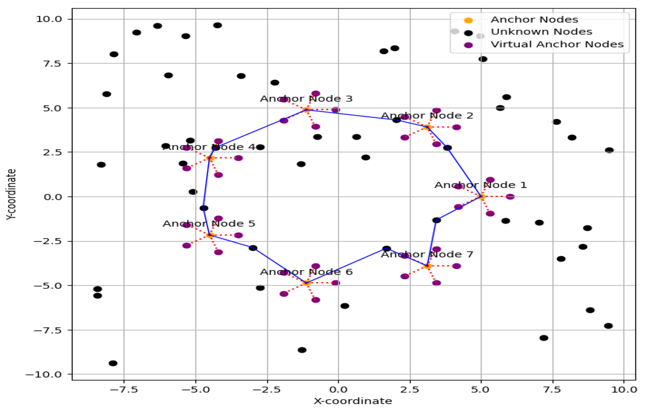
In the subsequent steps, we will consider a similar strategy, implementing data augmentation to augment the dataset as shown in Algorithm 1. We initiate by collecting a dataset of real anchor node positions. Through GAN training, the generator learns to create synthetic anchor positions that closely resemble a real location, while the discriminator distinguishes between real and synthetic positions. This training process ensures the generation of high-quality synthetic data. Therefore, we have considered multiple duplicates of virtual anchors positioned surrounding each original anchor, as depicted in Figure 2. The mathematical representation of the coordinates for these additional virtual anchors is governed by Equation (25). The main aim of the proposed augmentation technique is to implement an enhanced dataset, producing more versions of virtual anchors to alter the training data. The proposed scheme considers one hundred unknown nodes (U = 100) and seven anchor nodes (D = 7), and each anchor is encircled by five original virtual anchors (B = 5) as shown in Figure 3. The coordinates of the virtual anchors surrounded by the original anchor nodes can be formulated by developing a span range and multiplying it by a random Gaussian deviation $(\delta x_L,\delta y_L)$, represented as $(B_{cx},B_{cy})$, where $B_{cx}=Range\times$$randn(1,B)$ and $B_{cy}=Range\times$$randn(1,B)$ as shown in Algorithm 1. The positional coordinates of given anchor node i $(x_i,y_i)$ for (i = 1, …, D) and (L = 1, …, B) are given as:

$$\left.\begin{array}{ccc}(x_i\pm \delta x_1,x_i\pm \delta y_2)& =& (x_1,y_1)\\ (x_i\pm \delta x_2,x_i\pm \delta y_2)& =& (x_2,y_2)\\ \cdots & & \\ ⋮& & \\ (x_i\pm \delta x_L,x_L\pm \delta y_L)& =& (x_L,y_L)\end{array}\right\}$$

(25)

where D and B denotes the number of original and virtual deployed anchor nodes.

Algorithm 1 Pseudocode for the DAS algorithm

Input: Length of Border, Total Nodes, Anchor Nodes, Span Range, B; G (generation of coordinates of all nodes); Anchor = [G(1,1:Anchor Nodes);G(2,1:Anchor Nodes)]; Output:      1: Start    2: $B\leftarrow 5$    3: $L\leftarrow \mathrm{Anchor}\text{\_}\mathrm{Nodes}\times B$    4: for $i\leftarrow \mathrm{Total}\text{\_}\mathrm{Nodes}$ to $\mathrm{Anchor}\text{\_}\mathrm{Nodes}+1$ do    5:     Shift_unknown_nodes    6:     $n\leftarrow 1$    7:     for $j\leftarrow 1$ to $L+\mathrm{Anchor}\text{\_}\mathrm{Nodes}$ do    8:        $Bcx\leftarrow \mathrm{Range}\times \mathrm{randn}(1,B)$    9:        $Bcy\leftarrow \mathrm{Range}\times \mathrm{randn}(1,B)$  10:        for $k\leftarrow 0$ to B do  11:            if $k==0$ then  12:                Set $G1$  13:            else  14:                Bind $G(:,i+j)$  15:            end if  16:            Increment n  17:            Set $n\leftarrow n-1$  18:        end for  19:     end for  20: end for  21: End

The size of training data ${\left(Dis\right)}_T$ is given in the equation:

$${\left(Dis\right)}_T=(D\ast B+D)\ast U$$

(26)

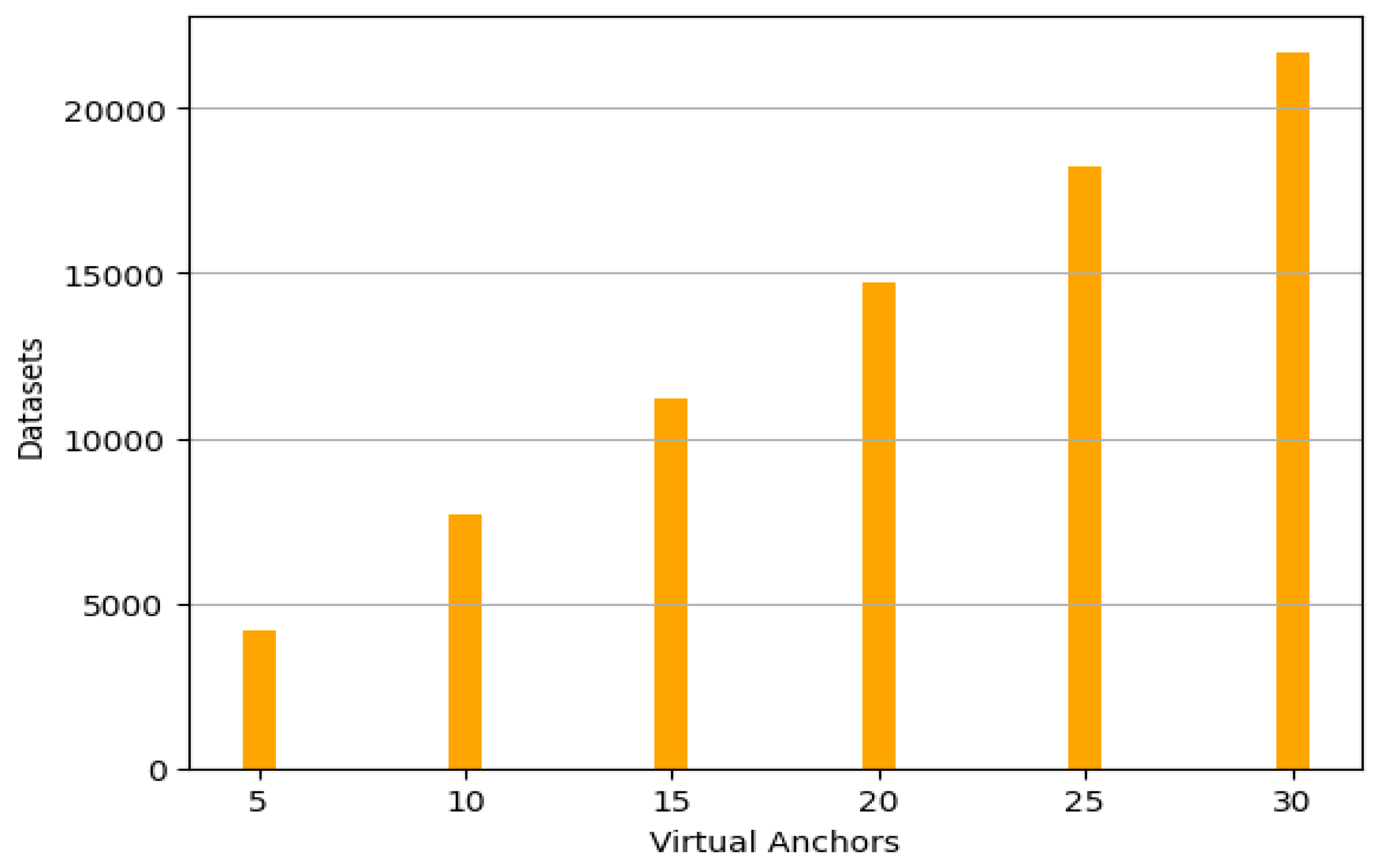
By taking the reference of Figure 3, the present scenario determines the composition of datasets by considering the number of the original anchors (D = 7), the number of unknown nodes (U = 100), and the presence of the virtual anchor nodes (B = 5). The total data size is estimated as 4200. Furthermore, increasing the size of virtual anchor nodes will result in a significant expansion of the overall data size as shown in Figure 3.

Next, the training and testing of these datasets will go through a deep neural network (DNN). Through a process of supervised learning, the DNN learns the detailed structure and correlations built in these sensor readings that enhance the actual distances.

Initially during the training step, the DNN generates its internal parameters through the optimization technique, aiming to minimize the error between estimated distances and ground level real values. This approach enables the DNN to generate a deep understanding of the complex mapping between the data calculated from sensors and real distances, capturing variations in the datasets and irregularities that may occur in the localization process.

The proposed DNN architecture consists of one input layer; five hidden layers with neuron counts of 30, 15, 10, 15, and 30; and a single output layer. During training, the adam optimizer is used to adjust weights repeatedly with the aim of optimizing model performance. Once trained, the DNN can efficiently estimate the distance of unknown nodes that are linked with the original anchor and virtual anchor nodes. When a newly deployed node enters the network or requires localization, the sensor node starts communicating data to the DNN, which then processes this information through its training and skilled model. The dataset is partitioned into 80% for training and 20% for the testing. The training of the DNN involves iterating up to 1100 times, a significant step taken to manage the DNN in achieving an optimal normalized mean-square error (MSE). By calculating the sensor readings with regard to the patterns learned during the training process, the DNN measures an estimate of the node’s distance from the anchor nodes in the network as shown in Algorithm 2.

Algorithm 2 DNN for distance estimation

1: function forward_pass(X):   2:     $H\leftarrow \mathrm{activation}\text{\_}\mathrm{function}(X\times W_1+b_1)$   3:     $Y\leftarrow \mathrm{activation}\text{\_}\mathrm{function}(H\times W_2+b_2)$   4:     return Y   5:     6: function train_DNN($X_{\mathrm{train}}$, $Y_{\mathrm{train}}$, $0.001$, 1100):   7:     initialize_parameters()   8: for  $epoch$  in  $[1,\dots ,1100]$  do   9:     for i in $[1,\dots ,\mathrm{len}\left(X_{\mathrm{train}}\right)]$ do 10:        $Y_{\mathrm{pred}}\leftarrow \mathrm{forward}\text{\_}\mathrm{pass}\left(X_{\mathrm{train}}\left[i\right]\right)$ 11:        $loss\leftarrow \mathrm{compute}\text{\_}\mathrm{loss}(Y_{\mathrm{pred}},Y_{\mathrm{train}}\left[i\right])$ 12:        compute_gradients($X_{\mathrm{train}}\left[i\right]$, $Y_{\mathrm{train}}\left[i\right]$, $Y_{\mathrm{pred}}$) 13:        update_weights($0.001$) 14:     end for 15: end for 16:   17: function activation_function(Z): 18:     return ReLU(Z) 19:   20: function ReLU(Z): 21:     return $\max (0,Z)$

6. Results and Analysis

The performance of the suggested algorithm is analyzed by simulation results by modifying the various parameters. The various parameters whose values are varied are node density, anchor density, virtual anchor nodes and transmission range.

Table 2. Parameters used in simulation.

Simulation Configuration	Value
WSN coverage region	$100\times 100$ m2
Transmission range	15 m, 20 m, 25 m, 30 m, 35 m
Unknown nodes	50
Anchor nodes	6
Virtual anchor nodes	5, 10, 15, 20, 25, 30
Span	2 m, 4 m, 6 m, 8 m, 10 m, 12 m
Optimization technique	Whale optimization

represents the simulation parameters, and the 100 × 100 m² area is taken for data simulation. To implement this strategy, we have considered two scenarios with different span ranges. The first scenario shows an illustration of 50 unidentified nodes followed by 6 anchor nodes, each encircled by 5 virtual anchors, with range of 2 m as shown in Figure 4a. The second scenario shows a uniform distribution of 50 unidentified nodes followed by 6 anchor nodes, each encircled by 5 additional virtual anchors, with a span range of 6 m shown in Figure 4b.

To verify the outcomes of the proposed algorithm with traditional DV-Hop methods, the localization error is calculated as the root-mean-square error (RMSE) shown in the equation given below:

$$\left(RMSE\right)=\frac{{\sum }_{p=1}^Q\sqrt{{(x^{cal}-x^{act})}^2+{(y^{cal}-y^{act})}^2}}{Q\times T}$$

(27)

where ($x^{cal}$, $y^{cal}$) and ($x^{act}$, $y^{act}$) denote the measured and actual position of unknown node.

6.1. The Impact of the Number of Virtual Anchors on Localization Error

Figure 5 depicts the relationship between localization error and virtual anchor nodes’ variation. The 100 × 100 m² area is examined for simulation purposes, where 50 unidentified nodes having a 25 m range among the sensor nodes are deployed within the network. Virtually deployed anchors are taken between 5 and 30. The simulation findings suggest that with an increase in the number of virtual anchor nodes, the localization error diminishes as clearly shown by Figure 5. Furthermore, it has come to our attention that the localization error of the proposed DNN-based DV-Hop outperforms other localization techniques.

6.2. The Impact of Span on Localization Error

The graph depicting the relationship between localization error and the span is presented in Figure 6. For simulation purposes, a 100 × 100 m² area is considered, where 50 unknown nodes, each with a transmission range of 25 m, are deployed. The virtual anchors are surrounded by real anchor nodes, and spans are taken between 2 and 12. We observe that with an increasing span, the localization error decreases, as clearly shown by Figure 6. This is due to the fact that a wider span between virtual anchor nodes can lead to better network connectivity, as it ensures that a larger portion of the network is covered by the anchor nodes. The proposed algorithm showcases increasing excellence over the DV-Hop approach as the span (distance) increases.

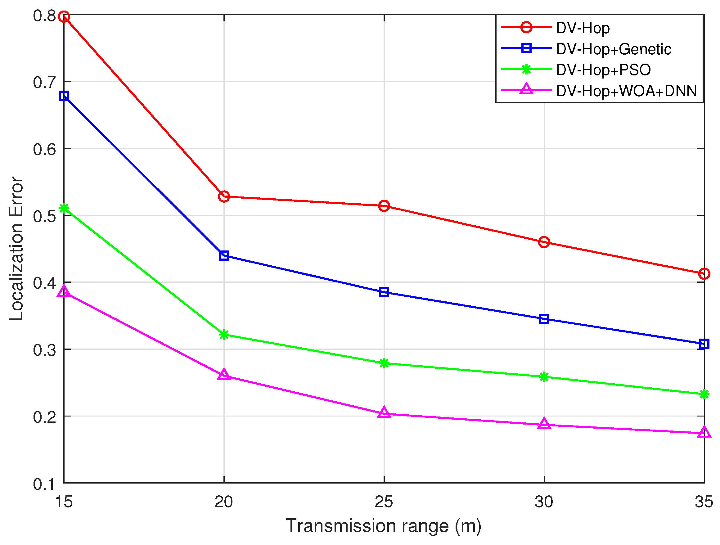
6.3. The Impact of Transmission Range on Localization Error

Impact of variability in transmission range on localization error is represented by Figure 7. A region spanning of 100 × 100 m² hosting a fixed complement of 50 unidentified nodes and seven anchors is taken for simulation purposes. Each anchor node is surrounded by five virtual anchor nodes. The transmission range is maintained within the range from 15 m to 35 m. Simulation results give evidence that localization error is reduced with regard to the higher value of the transmission range. The explanation for this is that when transmission range increases while unknown and anchor nodes are constant, the connectivity between the nodes is improved. Therefore, neighboring anchor nodes per unknown node rise. Therefore, the localization error decreases significantly with the increase in transmission range. As illustrated in Figure 7, we compared our proposed algorithm with traditional DV-Hop, genetic-based DV-Hop, and PSO-based DV-Hop algorithms. The analysis concluded that our proposed algorithm outperforms these algorithms.

6.4. The Impact of Span Variation on Localization Accuracy in DV-Hop and DV-Hop+WOA+DNN Algorithm

The examination of the traditional DV-Hop and proposed DNN approach involved systematically adjusting the span values to 2, 4, 6, 8 and 10, as shown in Figure 8 and Figure 9. As shown in the bar graph, there is a noticeable trend of increasing localization accuracy as the span distance and the number of virtual anchors are incremented. In this evaluation, we considered a range of virtual anchors (5, 10, 15, 20, 25) m and span distances ranging from 2 to 10 (m). This comprehensive analysis provides valuable insights into the effectiveness of our proposed DV-Hop DNN algorithm compared to the traditional DV-Hop method, highlighting its superior performance in achieving an accurate localization approach for the given scenario.

7. Conclusions

This paper presents a data augmentation strategy that enhances the number of additional added virtual anchors, substantially expanding the training dataset and leading to more precise localization. The proposed algorithm involves creating virtual anchors strategically around real anchors, thereby generating additional training data and significantly enhancing dataset size. However, deploying a large number of real anchor sensors can be impractical and present difficulties related to the availability of sufficient training data. In response to this challenge, we proposed a data augmentation scheme aimed at virtually expanding the anchor pool, thereby alleviating the financial constraints associated with deploying numerous physical anchors. Additionally, we have proposed a deep neural network algorithm to estimate the location of unidentified nodes. Simulation results show that our proposed algorithm achieves a reduction in localization error of approximately 33% compared to the traditional DV-Hop algorithm.

References

- Kumar, R.; Kumar, S.; Shukla, D.; Raw, R.S.; Kaiwartya, O. Geometrical Localization Algorithm for Three Dimensional Wireless Sensor Networks. Wirel. Pers. Commun. 2014, 79, 249–264. [Google Scholar] [CrossRef]
- Zou, D.; Sun, G.; Li, Z.; Xi, G.; Wang, L. Incremental Strategy-based Residual Regression Networks for Node Localization in Wireless Sensor Networks. KSII Trans. Internet Inf. Syst. 2022, 16, 2627–2647. [Google Scholar] [CrossRef]
- Cortez-González, J.; Ruiz-Ibarra, E.; Espinoza-Ruiz, A.; Castro, L.A.; Mass-Sanchez, J. Weighted Hyperbolic DV-Hop Positioning Node Localization Algorithm in WSNs. Wirel. Pers. Commun. 2016, 96, 5011–5033. [Google Scholar] [CrossRef]
- Gupta, V.; Singh, B. Study of range free centroid based localization algorithm and its improvement using particle swarm optimization for wireless sensor networks under log normal shadowing. Int. J. Inf. Technol. 2018, 12, 975–981. [Google Scholar] [CrossRef]
- Gao, W.; Ge, Y.; Wang, S.; Li, Y.; Lou, K.; Jiang, M.; Jiang, J. Improved DV-Hop Localization Algorithm Based on Anchor Weight and Distance Compensation in Wireless Sensor Network. Int. J. Signal Process. Image Process. Pattern Recognit. 2017, 9, 167–176. [Google Scholar] [CrossRef]
- Gui, L.; Zhang, X.; Ding, Q.; Shu, F.; Wei, A. Reference Anchor Selection and Global Optimized Solution for DV-Hop Localization in Wireless Sensor Networks. Wirel. Pers. Commun. 2017, 96, 5995–6005. [Google Scholar] [CrossRef]
- Pandey, S.; Varma, S. A Range Based Localization System in Multihop Wireless Sensor Networks: A Distributed Cooperative Approach. Wirel. Pers. Commun. 2016, 86, 615–634. [Google Scholar] [CrossRef]
- Rashid, H.; Turuk, A.K. Localization of wireless sensor networks using a single anchor node. Wirel. Pers. Commun. 2013, 72, 975–986. [Google Scholar] [CrossRef]
- Kanwar, V.; Kumar, A. Multiobjective optimization-based DV-hop localization using NSGA-II algorithm for wireless sensor networks. Int. J. Commun. Syst. 2020, 33, e4431. [Google Scholar] [CrossRef]
- Najeh, T.; Sassi, H.; Liouane, N. A Novel Range Free Localization Algorithm in Wireless Sensor Networks Based on Connectivity and Genetic Algorithms. Int. J. Wirel. Inf. Netw. 2018, 25, 88–97. [Google Scholar] [CrossRef]
- Kumar, G.; Rai, M.K.; Saha, R.; Kim, H.J. An improved DV-Hop localization with minimum connected dominating set for mobile nodes in wireless sensor networks. Int. J. Distrib. Sens. Netw. 2018, 14, 2018. [Google Scholar] [CrossRef]
- Mekelleche, F.; Haffaf, H. Classification and comparison of range-based localization techniques in wireless sensor networks. J. Commun. 2017, 12, 221–227. [Google Scholar] [CrossRef]
- Yadav, P.; Kumar, K.; Sharma, S.C. Machine Learning Based Techniques for Node Localization in WSN: A Survey. In Proceedings of the International Conference on Device Intelligence, Computing and Communication Technologies, (DICCT), Dehradun, India, 17–18 March 2023; pp. 12–17. [Google Scholar] [CrossRef]
- Kumar, S.; Lobiyal, D.K. An Advanced DV-Hop Localization Algorithm for Wireless Sensor Networks. Wirel. Pers. Commun. 2013, 71, 1365–1385. [Google Scholar] [CrossRef]
- Chen, X.; Zhang, B. Improved DV-Hop node localization algorithm in wireless sensor networks. Int. J. Distrib. Sens. Netw. 2012, 8, 213980. [Google Scholar] [CrossRef]
- Zaidi, S.; El Assaf, A.; Affes, S.; Kandil, N. Range-free nodes localization in mobile wireless sensor networks. In Proceedings of the 2015 IEEE International Conference on Ubiquitous Wireless Broadband (ICUWB), Montreal, QC, Canada, 4–7 October 2015; pp. 1–6. [Google Scholar]
- Zazali, A.A.; Subramaniam, S.K.; Zukarnain, Z.A. Flood Control Distance Vector-Hop (FCDV-Hop) Localization in Wireless Sensor Networks. IEEE Access 2020, 8, 206592–206613. [Google Scholar] [CrossRef]
- Maddumabandara, A.; Leung, H.; Liu, M. Experimental Evaluation of Indoor Localization Using Wireless Sensor Networks. IEEE Sens. J. 2015, 15, 5228–5237. [Google Scholar] [CrossRef]
- Sharma, G.; Kumar, A. Improved range-free localization for three-dimensional wireless sensor networks using genetic algorithm. Comput. Electr. Eng. 2018, 72, 808–827. [Google Scholar] [CrossRef]
- Srinivas, M.; Patnaik, L.M. Genetic Algorithms: A Survey. Computer 1994, 27, 17–26. [Google Scholar] [CrossRef]
- Singh, S.P.; Sharma, S.C. Implementation of a PSO Based Improved Localization Algorithm for Wireless Sensor Networks. IETE J. Res. 2019, 65, 502–514. [Google Scholar] [CrossRef]
- Kaur, A.; Kumar, P.; Gupta, G.P. Nature Inspired Algorithm-Based Improved Variants of DV-Hop Algorithm for Randomly Deployed 2D and 3D Wireless Sensor Networks. Wirel. Pers. Commun. 2018, 101, 567–582. [Google Scholar] [CrossRef]
- Sugasaki, M.; Shimosaka, M. Robustifying Wi-Fi Localization by Between-Location Data Augmentation. IEEE Sens. J. 2022, 22, 5407–5416. [Google Scholar] [CrossRef]
- Marquez, L.E.; Calle, M. Machine learning for localization in LoRaWAN: A case study with data augmentation. In Proceedings of the IEEE Future Networks World Forum (FNWF), Montreal, QC, Canada, 10–14 October 2022; pp. 422–427. [Google Scholar] [CrossRef]
- Faheem, M.; Kuusniemi, H.; Eltahawy, B.; Bhutta, M.S.; Raza, B. A lightweight smart contracts framework for blockchain-based secure communication in smart grid applications. IET Gener. Transm. Distrib. 2024, 18, 625–638. [Google Scholar] [CrossRef]
- Raza, B.; Aslam, A.; Sher, A.; Malik, A.K.; Faheem, M. Autonomic performance prediction framework for data warehouse queries using lazy learning approach. Appl. Soft Comput. J. 2020, 91, 106216. [Google Scholar] [CrossRef]
- Sharma, G.; Kumar, A. Improved DV-Hop localization algorithm using teaching learning based optimization for wireless sensor networks. Telecommun. Syst. 2017, 67, 163–178. [Google Scholar] [CrossRef]
- Kanwar, V.; Kumar, A. DV-Hop-based range-free localization algorithm for wireless sensor network using runner-root optimization. J. Supercomput. 2020, 77, 3044–3061. [Google Scholar] [CrossRef]
- Bozorgi, S.M.; Yazdani, S. IWOA: An improved whale optimization algorithm for optimization problems. J. Comput. Des. Eng. 2019, 6, 243–259. [Google Scholar] [CrossRef]
- Njima, W.; Chafii, M.; Chorti, A.; Shubair, R.M.; Poor, H.V. Indoor Localization Using Data Augmentation via Selective Generative Adversarial Networks. IEEE Access 2021, 9, 98337–98347. [Google Scholar] [CrossRef]
- Wu, X.; Zhang, Y.; Yu, J.; Zhang, C.; Qiao, H.; Wu, Y.; Wang, X.; Wu, Z.; Duan, H. Virtual data augmentation method for reaction prediction. Sci. Rep. 2022, 12, 17098. [Google Scholar] [CrossRef]
- Chen, Y.; Li, G.; Tan, Y.; Zhang, G. Graph-Based Radio Fingerprint Augmentation for Deep-Learning-Based Indoor Localization. IEEE Sens. J. 2023, 23, 6074–6084. [Google Scholar] [CrossRef]
- Esheh, J.; Affes, S. Effectiveness of Data Augmentation for Localization in WSNs Using Deep Learning for the Internet of Things. Sensors 2024, 24, 430. [Google Scholar] [CrossRef]
Figure 1.
Flow chart for DV-Hop algorithm.
Figure 2.
Deployment of virtual anchor nodes.
Figure 3.
Datasets of virtual augmentation strategy.
Figure 4.
(a) Sensor node deployment with a span of 2 m (b) Sensor node deployment with a span of 6 m.
Figure 5.
Localization error versus virtual anchors.
Figure 6.
Localization error versus span.
Figure 7.
Error in localization plotted against transmission range.
Figure 8.
Span variation in DV-Hop algorithm.
Figure 9.
Span variation in DV-Hop+WOA+DNN algorithm.