
Wind Power Forecasting with Machine Learning Algorithms in Low-Cost Devices
by
 , , and
Pablo Andrés Buestán-Andrade
1,* ,
,
Mario Peñacoba-Yagüe
2,*,
Jesus Enrique Sierra-García
2 and
Matilde Santos
3
1
Computer Science Faculty, Complutense University of Madrid, 28040 Madrid, Spain
2
Department of Digitalization, University of Burgos, 09006 Burgos, Spain
3
Institute of Knowledge Technology, University Complutense of Madrid, 28040 Madrid, Spain
*
Authors to whom correspondence should be addressed.
Electronics 2024, 13(8), 1541; https://doi.org/10.3390/electronics13081541
Submission received: 29 February 2024
/
Revised: 10 April 2024
/
Accepted: 15 April 2024
/
Published: 18 April 2024
(This article belongs to the Special Issue Application of Time Series Analysis and Forecasting in Computer Science)
Abstract
:The urgent imperative to mitigate carbon dioxide (CO2) emissions from power generation poses a pressing challenge for contemporary society. In response, there is a critical need to intensify efforts to improve the efficiency of clean energy sources and expand their use, including wind energy. Within this field, it is necessary to address the variability inherent to the wind resource with the application of prediction methodologies that allow production to be managed. At the same time, to extend its use, this clean energy should be made accessible to everyone, including on a small scale, boosting devices that are affordable for individuals, such as Raspberry and other low-cost hardware platforms. This study is designed to evaluate the effectiveness of various machine learning (ML) algorithms, with special emphasis on deep learning models, in accurately forecasting the power output of wind turbines. Specifically, this research deals with convolutional neural networks (CNN), fully connected networks (FC), gated recurrent unit cells (GRU), and transformer-based models. However, the main objective of this work is to analyze the feasibility of deploying these architectures on various computing platforms, comparing their performance both on conventional computing systems and on other lower-cost alternatives, such as Raspberry Pi 3, in order to make them more accessible for the management of this energy generation. Through training and a rigorous benchmarking process, considering accuracy, real-time performance, and energy consumption, this study identifies the optimal technique to accurately model such real-time series data related to wind energy production, and evaluates the hardware implementation of the studied models. Importantly, our findings demonstrate that effective wind power forecasting can be achieved on low-cost hardware platforms, highlighting the potential for widespread adoption and the personal management of wind power generation, thus representing a fundamental step towards the democratization of clean energy technologies.
1. Introduction
Wind power is increasingly recognized as a pivotal component in the global effort to transition towards sustainable energy solutions amidst escalating concerns regarding climate change and the imperative to mitigate greenhouse gas emissions [1]. The utilization of wind turbines for electricity generation has gained significant attention due to their clean nature and potential to contribute to decarbonization efforts [2].
However, the inherent variability of the wind resource poses challenges in terms of efficiency and reliability in power generation, as well as its integration into the electrical grid [3]. This is why the forecasting of variables such as wind speed and energy production has become crucially important. The ability to accurately predict these variables not only enhances the operational efficiency of wind farms but also enables better control systems and the implementation of predictive maintenance strategies, which can reduce operational costs and increase the technology’s lifespan.
However, nowadays, new regulations are fostering the use of clean energy at any level, even the isolated installation of small wind turbines that are intended to cover for individual energy consumption. This generalization of the use of the renewable devices demands affordable energy management. If their wind energy generation has to be reliable, consumers must have access to tools that allow them to plan and handle the power produced by the wind converters. Thus, low-cost solutions for the prediction of energy generation are a must. This will allow consumers to better plan energy buying from the electric grid, reduce costs, and avoid energy wasting.
In this work, in order to improve the accuracy and efficiency of predictions in the context of wind energy, various machine learning model architectures have been applied and implemented. Among others, we have considered convolutional neural networks (CNNs), long short-term memory (LSTM) neural networks, gated recurrent unit (GRU) cells, and transformers, which are all particularly suited for processing temporal series of data. This research evaluates and compares these machine learning models implemented on low-cost devices. Training and test experiments have been carried out to identify the most suitable model architecture to effectively address the forecasting of wind power generation.
The implementation of these machine learning techniques on different hardware platforms has been analyzed with the aim of finding affordable and low-cost solutions that can be proposed to energy consumers. These novel techniques have been designed to run smoothly on cost-effective systems, defined as hardware platforms that are economically accessible to a wide range of users, typically priced below EUR 100. This definition of low-cost devices covers devices like the Raspberry Pi 3 (Raspberry Pi foundation, Cambridge, UK).
The implementation of these techniques in low-cost devices has many advantages, not only at the level of use but also in engineering education and to address some challenges that Industry 4.0 brings [4]. Therefore, the importance of and need to use low-cost hardware platforms in wind energy prediction cannot be underestimated if the use of this type of renewable energy is to be extended. These platforms offer accessibility to cutting-edge advances in wind resource prediction technology for researchers, educators, and professionals in the sector. On the other hand, using low-cost platforms to provide solutions that improve energy generation allows for democratizing the use of these wind devices, allowing entities and individuals with limited resources to benefit from this energy source, as well as its possible extension to other applications.
To summarize, the final goal of this experimental study is to analyze the potential for cost-effective computing solutions, such as the Raspberry Pi 3, to make advanced machine learning algorithms more accessible to individuals and for small-scale applications, such as wind energy generation on low-cost devices, thus expanding their use.
The main contributions of this paper can be stated as follows:
- I.
- This study works with different machine learning techniques for wind forecasting using real-time series wind data, considering factors such as the data window size and the input features. It systematically evaluates different deep learning methodologies (CNN, FC), including some more recent ones such as GRU and transformers;
- II.
- This research also investigates the impact on the training process of the algorithms, which used a novel filtering method integrated into the input feature set of the temporal series;
- III.
- The evaluation of machine learning (ML) models, carried out through metrics such as the root mean square error (RMSE) and mean absolute error (MAE) of different variables, such as accuracy;
- IV.
- The feasibility of implementing these ML forecasting techniques in diverse computing platforms is explored, comparing their performance on both conventional computing systems and more cost-effective alternatives, such as Raspberry Pi 3, and considering the accuracy, real-time performance, and energy consumption on both types of platforms.
This work is structured as follows: the following section gives an overview of the state of the art on wind power forecasting using different platforms. In Section 3, the machine learning techniques used herein for wind energy prediction are presented, detailing their configuration. The experiments carried out and the results obtained are described and discussed in Section 4. Finally, the conclusions and potential future research directions are mentioned.
2. Related Works
Advanced machine learning algorithms play a key role in wind forecasting due to their ability to capture complex patterns and non-linear relationships in wind data [5]. These algorithms, such as recurrent neural networks (RNNs), gated recurrent units (GRUs), and transformer models, have proved successful in sequential data prediction, making them well-suited for wind power time series forecasting. RNNs, including GRU architectures, are particularly adapted to modeling temporal dependencies in wind data, while transformer-based models, originally developed for natural language processing, have shown promising results in various time series forecasting applications [6]. The utilization of these advanced machine learning algorithms not only enhances the accuracy of wind forecasting but also enables the identification of subtle patterns and trends that traditional statistical methods may overlook [7]. As an example of these algorithms’ utilization, Zhang et al. 2019 [8] carried out a study in which the LSTM network was applied to forecast the output power from a wind farm situated in China. The input data consisted of three months’ wind speed data obtained from numerical weather prediction (NWP) models, while the wind power that was generated served as the output variable. Another interesting paper is [9], in which a comparison between LSTM and GRU techniques’ use for short-term offshore wind speed forecasting was performed. Another comparative study is presented in [10], where the efficacy of the LSTM, GRU, and transformer neural network architectures for predicting wind turbine variables is analyzed. The findings of this paper show the superior adaptability of the GRU model to time series data, as evidenced by its lower RMSE and MAE errors compared to the LSTM and transformer architectures. Moreover, this study emphasized the importance of integrating additional features to enhance the predictive capabilities of machine learning models.
As this study focuses on low-cost hardware implementation, it is worth mentioning that low-cost technology has gained importance for sensors, both physical and virtual (IoT), that monitor devices and measure variables, especially those related to the weather. However, far fewer works explore low-cost solutions for prediction. This is due to the heavy computational load of some intelligent techniques, such as neural networks in general and, particularly, deep learning networks, which require substantial computation and memory resources. There are different approaches to addressing this issue. One solution is to use hardware-based neural networks. In [11], recent advances in light-weight deep learning models and network architecture search (NAS) algorithms are reviewed, starting with simplified layers and efficient convolution and including new architectural designs and optimization. Several practical applications of efficient CNNs have been investigated using various types of hardware architectures and platforms. In [12], the hardware implementation of different complex machine learning models such as convolutional neural networks (CNNs), recurrent neural networks (RNNs), and artificial neural network (ANNs) is investigated. The challenges, such as speed, area, resource consumption, and throughput, are discussed. In [13], a new framework for end-to-end deep neural networks’ training, quantization, and deployment is presented. The proposal is compared to existing embedded inference engines in terms of memory and power efficiency.
In any case, the most common approach is to simplify the neural network so as to be able to implement it on a small computational device. For instance, in [14], the authors propose an area-efficient implementation of an artificial neural network, reducing the number of layers in the ANN by nearly half, and keeping the number of fixed layers as low as possible. This way, they use less area to minimize the cost of on-chip implementation. Among the less-demanding NNs, spiking neural networks (SNN) have attracted much attention regarding hardware implementations, mainly in the neuromorphic hardware research community, as they are neuromorphic systems based on the information processing and storage procedure of biological neurons. In [15], a low-cost and high-speed implementation of a spiking neural network based on FPGA is proposed. Also, in [16], the current implementations of SNNs on various hardware platforms are discussed.
In [17], a lightweight convolutional neural network, TripleNet, is designed where the network model reduces the number of parameters of the network so it can operate easily on Raspberry Pi to perform image classification experiments. A simplified CNN was implemented in a drowsiness driving detection system using Raspberry Pi in [18].
Furthermore, Table 1 presents a selection of references that have used low-cost hardware platforms to implement machine learning algorithms, which allows us to highlight the differences in our article. These references have been found using the Google Scholar database with the following search terms: “Deep learning on a Raspberry PI”, “CNN on low-cost hardware”, “CNN on Raspberry Pi”, and “Neural networks on low-cost hardware”. These studies exemplify the potential of low-cost hardware to drive innovation and address real-world challenges using advanced and intelligent techniques. The objective of this summary is to provide information on the growing trend of using low-cost hardware for machine learning applications for various applications. To the best of our knowledge, this is the first study that evaluates wind energy forecasting based on low-cost hardware platforms.
Inspired by these articles, the present research aims to further explore advanced machine learning techniques and their potential application to improve the accuracy of wind energy prediction, using a practical approach that has not been covered in the mentioned articles. This approach is the hardware implementation of these ML techniques for time series prediction on low-cost platforms, with a novel objective of making them accessible and affordable for any wind turbine owner.
3. Machine Learning Techniques
Before describing the configuration, training, and validation of the proposed machine learning models, a brief overview of the techniques used in this study is presented. These techniques are CNN, fully connected, GRU, and transformer models.
3.1. CNN
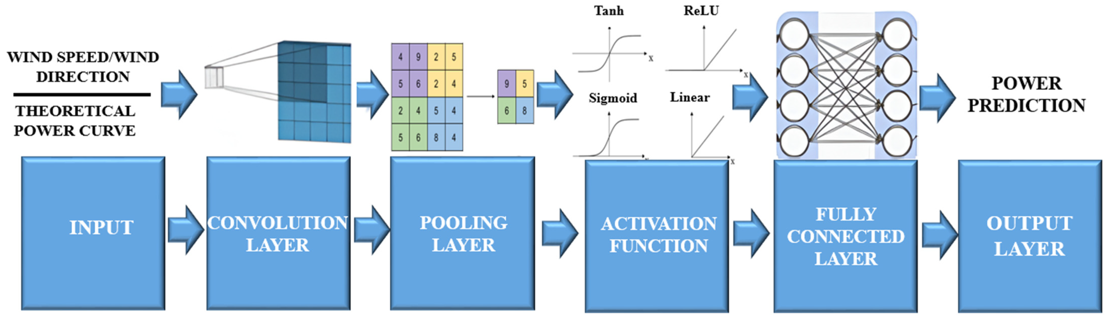
CNNs are a class of deep feedforward neural networks characterized by their convolutional structure, and primarily used through supervised learning methodologies. Moreover, their architecture encompasses convolutional, pooling, and fully connected layers [25]. These layers play key roles in feature extraction within the CNN framework. The convolutional layer processes input features through convolutions, extracting spatial patterns for subsequent analysis. Following this, the pooling layer aggregates information from preceding convolutional layers while reducing its spatial dimensions. Finally, the fully connected layer transforms the two-dimensional features into one-dimensional data for output representation. Figure 1 shows the CNN architecture used in this research.
The components of the CNN architecture (Figure 1) are described as follows:
- Convolutional Layers: Convolutional layers are the core of CNNs and extract spatial features from the input data. For wind energy prediction, these layers capture complex relationships between wind patterns and their impact on turbine performance. By traversing the spatial grid of the sensor data, convolutional filters capture localized patterns that are essential to their power prediction function. Within this component of the CNN architecture, it is important to analyze the “kernel size”. This parameter determines the dimensions of the filters used in the convolutional layers. For example, a kernel size of three means that the filters have a spatial dimension of 3 × 3 pixels or elements. This dimension determines the receptive field of each filter and influences the granularity of the features extracted from the input data. Another relevant parameter is the number of neurons or units in each layer. This parameter influences the network’s ability to learn and represent complex relationships underlying the data. Furthermore, the convolutional layers are influenced by the number of filters or kernels in each convolutional layer of the neural network. Filters are small spatial windows of the input data that extract relevant features. In this context, with 128 filters, the convolutional layers of the network are capable of capturing a wide range of spatial patterns and features from the input data.
- Pooling Layers: Integrating pooling layers into CNN architectures enables the reduction of spatial dimensions within feature maps, facilitating the extraction of essential information while mitigating the computational complexity. This has been implemented by the “Pool_size” parameter, which specifies the size of the pooling window used for downsampling. As an example, a pool size of three indicates that the pooling operation is applied over non-overlapping windows of size 3 × 3, effectively reducing the spatial dimensions of the feature maps by a factor of three.
- Activation Functions: Employing non-linear activation functions, such as rectified linear units (ReLU), empowers CNNs to model complex relationships between input variables and the predicted power output. The activation method used with this technique is denoted by the term “Activation”. This parameter governs how neurons process and propagate information. Moreover, “Relu” refers to the rectified linear unit activation function, which introduces non-linearity into the network by outputting the input directly if it is positive, and zero otherwise. On the contrary, “Leaky_relu” refers to the leaky rectified linear unit activation function, which is similar to the traditional ReLU function but allows for a small, non-zero gradient when the input is negative. The latter, which helps alleviate the vanishing gradient problem and facilitates better training stability and convergence, was implemented in the fully connected method.
- Fully Connected Layers: Following the convolutional and pooling layers, fully connected layers integrate extracted spatial features to generate final model outputs. These layers use the information obtained from the convolutional operations to discern relationships between the input and output, that is, the wind dynamics and turbine performance in our case.
- Output Layers: To improve the generalization ability of CNNs, regularization techniques such as dropout and weight decay are commonly employed. Introducing noise or constraints during training helps avoid overfitting and promotes the development of more accurate models for prediction.
3.2. Fully Connected
The fully connected (FC) model is a neural network architecture characterized by a dense interconnection between neurons along consecutive layers. In this model, each neuron in a given layer is connected to every neuron in the subsequent layer, facilitating comprehensive information exchange throughout the network.
At its core, the FC model consists of multiple layers: an input layer, one or more hidden layers, and an output layer. Each layer has neurons, or nodes, which perform computations on the incoming data and pass the results to the neurons in the subsequent layer (Figure 2).
The input layer receives the raw input data, which could be in the form of feature vectors or flattened representations of multidimensional data. Each neuron in the input layer corresponds to a specific feature or attribute of the input data.
The hidden layers, situated between the input and output layers, perform the bulk of the computation in the FC model. Neurons in these layers apply linear transformations to the input data using weighted connections and activation functions, thereby extracting increasingly abstract representations of the input.
The output layer generates the final predictions or classifications based on the processed information from the hidden layers. The number of neurons in the output layer corresponds to the number of output classes or the dimensionality of the prediction space.
During its training, the FC model learns to adjust the weights associated with each connection between neurons using optimization algorithms such as gradient descent. This process aims to minimize the discrepancy between the model’s predictions and the ground truth labels in the training data.
To prevent overfitting and improve its generalization performance, regularization techniques such as dropout, weight decay, and early stopping are commonly applied to the FC model. These techniques help to control the complexity of the model and ensure that it can effectively generalize to unseen data.
The flexibility and adaptability of the fully connected model make it well-suited for a wide range of tasks, including regression, classification, and pattern recognition. While it may not be as efficient in handling high-dimensional data with spatial dependencies as other architectures, like convolutional neural networks (CNNs), the FC model remains a fundamental building block in the field of deep learning.
3.3. GRU
Gated recurrent unit (GRU) cell networks, similarly to the long short-term memory (LSTM) neural networks, constitute a compelling alternative that addresses the shortcomings of traditional recurrent neural networks (RNNs) while offering computational efficiency and architectural simplicity. Like LSTM, the GRU method is designed to avoid the issue of vanishing gradients and ineffective long-term information retention in sequential data processing [8]. However, the GRU method distinguishes itself by introducing two gates: the update gate and the reset gate [28]. These gates serve as dynamic controllers, regulating the flow of information throughout the network and enabling selective information retention and propagation. The update gate determines the proportion of new information to be incorporated into the memory cell, striking a delicate balance between preserving past information and incorporating novel knowledge (Figure 3). Meanwhile, the reset gate dictates the extent to which historical information influences the current state, allowing the GRU method to adaptively adjust its behavior based on the contextual relevance of past observations. By strategically integrating these gating mechanisms into its architecture, the GRU method achieves a fine-grained control over the information flow, effectively mitigating the challenge of gradient vanishing and facilitating the seamless propagation of relevant information across time series [29]. This elegant design not only enhances the model’s ability to capture long-term dependencies but also streamlines the computational burden associated with training recurrent neural networks, making the GRU method a good choice for a wide range of sequential data processing tasks, including natural language processing, time series analysis, and speech recognition.
The main difference between the GRU and LSTM models is that the GRU model replaces the forget gate and input gate in LSTM neural networks with an update gate. Furthermore, it changes the cell state and hidden state () to merging. This feature enables GRU networks to have fewer parameters [30].
3.4. Transformer Model
The new transformer model paradigm changes the more traditional approach of recurrent neural networks (RNN) by adopting an encoder-decoder framework and changing the fundamental mechanisms underlying the information propagation and context modeling [32]. Within this architecture, the encoder module takes on the role of processing time series data, through interconnected layers, to obtain the sequential patterns. The input layer receives the raw temporal data, and the encoder organizes the interaction between the components, including a positional encoding layer, a self-attention mechanism, normalization layers, and fully connected layers. To define all these layers, a series of parameters has been established.
To quantify the number of attention heads used in the self-attention mechanism, “Num_heads” has been introduced as a parameter. Each attention head independently attends to different parts of the input sequence, allowing the model to capture various relationships and dependencies. Additionally, the number of units or neurons in the forward layers has been specified with “ff_dim”. A high value of this parameter implies a larger hidden layer size, allowing the model to learn more complex representations and interactions within the data. Finally, the “key_dim” parameter determines the dimensionality of the query, key, and value vectors used to calculate the attention scores. These vectors are linear projections of the inputs and are used to calculate the attention weights. A high “key_dim” value allows the model to capture more detailed relationships and dependencies within the input sequence.
This complex layer structure culminates in a high-dimensional vector representation of the essence of the temporal sequence. Subsequently, this encoded vector is transformed through the decoder module, where it serves as a basis for generating predictions of future values in an autoregressive manner. Mirroring the encoder architecture, the decoder module weaves together positional encoding, self-attention masks, normalization layers, and decoding-encoding attention layers to obtain time series predictions. At the heart of the transformer model are its attention mechanisms and positional encoding techniques. Attention mechanisms dynamically weight the importance of different elements of the input sequence, and positional coding provides sequential data with spatial information.
The architecture of the transformer model is shown in Figure 4.
4. Models Training
The comparative study of different machine learning architectures for wind power prediction presented herein considers data selection, preprocessing, and performance evaluation metrics. The dataset is used for model training and testing, and preprocessing techniques are crucial for enhancing the data quality and model performance. The predictive model’s precision is evaluated based on metrics such as the root mean square error (RMSE), mean absolute error (MAE), and mean absolute percentage error (MAPE), together with the evaluation of the model’s computational complexity in terms of its prediction speed, memory usage, and energy consumption on different platforms.
4.1. Dataset
The dataset comes from a wind turbine’s supervisory control and data acquisition (SCADA) system, which records several variables at 10 min intervals [33]. Specifically, it is obtained from a wind turbine situated in Turkey. The dataset includes the following variables:
- Date/Time: Recorded at 10 min intervals, this timestamp provides temporal context for each data point, enabling temporal analysis and trend identification;
- LV Active Power (kW): This variable denotes the actual power generated by the wind turbine at a specific moment in kilowatts (kW). It serves as a direct indicator of the turbine’s performance and output power efficiency;
- Wind Speed (m/s): Measured at the hub height of the turbine, this measurement represents the velocity of the wind, which is key for determining the turbine’s power generation capacity as it is proportional to the turbine’s ability to convert kinetic energy into electrical power;
- Theoretical_Power_Curve (KWh): This variable gives the theoretical power expected from the turbine at different wind speeds, as specified by the turbine manufacturer. It serves as a reference to evaluate the turbine’s actual performance against its designed capacity;
- Wind Direction (°): Recorded at the hub height of the turbine, this parameter indicates the direction from which the wind is blowing. Wind turbines automatically adjust their orientation to align with the prevailing wind direction (yaw control), optimizing energy capture.
To give a better explanation of the dataset, histograms of the wind speed, theoretical power curve, active power, and wind direction are shown in Figure 5, and the main parameters are summarized in Table 2.
The dataset helps to better understand the wind energy generation, facilitating in-depth analysis of factors influencing the turbine performance, such as the wind speed, direction, and misalignment, and their relationship with the actual power output.
4.2. Pre-Processing
The present research uses machine learning techniques to forecast the active power output of a 5 MW wind turbine located in Turkey. This is achieved by using data gathered via the SCADA system in 2018, with readings taken every 10 min. The dataset includes variables such as the wind speed, theoretical power curve, wind direction, and active power, with the latter being the primary variable of interest for analysis.
To address the complexity of the model and the interactions among these variables, a specific function was developed to explore all possible combinations of the variables as inputs for the machine learning model.
The variables were normalized by calculating their mean and dividing it by their standard deviation. This step is essential to standardize the scales of the variables, improving the convergence capability of machine learning algorithms during the training phase.
Finally, the dataset was split into three parts: 70% for training, 20% for validation, and 10% for testing. This division enabled a thorough assessment of the models’ performance and predictive ability across various scenarios.
4.3. Training Methodology
The training process of the techniques is as follows. Initially, the selection of the best configuration of each model for the specific objective herein proposed was obtained with the random search technique [34]. This approach systematically explores a wide range of potential hyperparameter combinations. It was applied to all of the deep learning models, the convolutional, GRU, transformer, and FC neural networks.
The hyperparameters of the configuration of each technique include:
- The number of layers of the network architecture;
- The number of filters in the convolutional layers;
- The size of the kernels that affect the input of the networks;
- The activation function that determines the output of the nodes;
- The pooling size, to reduce dimensionality;
- The dropout rate, to prevent overfitting;
- The input window size, essential in systems relying on temporal patterns.
The random search technique is known for its ability to explore the hyperparameter space more efficiently compared to exhaustive methods, such as grid search, especially when the number of hyperparameters is large. By selecting random combinations, it is possible to find near-optimal configurations with fewer computations, saving time and computational resources.
Table 3 shows the best hyperparameter found with the random search method for each machine learning technique.
The parameters listed in Table 3 provide some insights into the architecture of each neural network model, and into the structure and behavior of the networks, which influence their performance and capabilities. A brief mention of the general parameters (the ones used in every architecture) is given below. The hyperparameters that only affect a specific architecture have been explained in Section 3.
- Window: Refers to a parameter related to the input data or sequence. That is, it indicates the window size used for processing input data or sequences. For example, a window size of 20 means that the model considers the previous 20 samples as input features;
- Num_layers: Indicates the number of layers in the neural network. For instance, if the num_layers parameter is three, it means that the network has three layers stacked sequentially, each contributing to the hierarchical representation of the input data;
- Dropout rate: This is a hyperparameter used in regularization techniques. A dropout rate of 0.1 would mean that 10% of the neurons in each layer are randomly dropped out during training to prevent overfitting.
5. Experimental Setup
5.1. Hardware
In this study, we used two hardware platforms with different costs to show the versatility of our approach in accommodating for different economic scales. The first one is a Dell Vostro 5410 computer, positioned as a middle-cost computing solution, which is equipped with 8 GB of RAM and an eighth-generation Intel Core i7 processor running on the Windows operating system. The cost of this device falls within the range of EUR 300–EUR 1000 (EUR 700 approximately), representing a conventional computing environment with substantial computational resources.
The second platform is a Raspberry Pi 3 Model B, a low-cost hardware option priced under EUR 100, operating on a Linux system. This model has a 1.2 GHz 64-bit quad-core ARM Cortex-A53 processor and comes with 2 GB of RAM. The Raspberry Pi 3 was selected in order to show the potential of low-cost, more accessible platforms for implementing advanced machine learning algorithms. Moreover, it has been selected primarily due to its widespread popularity and the support it receives from a large and active community. This extended use ensures that a wealth of resources, tutorials, and troubleshooting information is available, which is a great help for implementing and optimizing machine learning algorithms. This strong support from a large community also facilitates easier replication of our research findings and broader applicability in diverse scenarios and applications, making it an ideal choice for our study [35]. Despite its much lower price and comparatively modest computational capacity, the Raspberry Pi 3 has proved effective at executing the predictive models obtained in our study.
Furthermore, working with platforms with different costs emphasizes the practicality and scalability of the implementation of machine learning solutions, in this case for energy forecasting, and includes the economic factor to make these tools more widely accessible.
5.2. Software
To implement the neural network models, a set of libraries based on TensorFlow (version 2.0) and Keras (version 2.13.1) was used. TensorFlow (version 2.0), an open-source library for numerical computing and machine learning, made it easy to build the multilayer neural networks. Keras, a high-level neural network API, was used for its simplicity, and to define and train the CNN, GRU, and transformer models.
MinMaxScaler from Scikit-learn was used for normalization, ensuring that the data were scaled to a uniform range. The Keras sequential model was instrumental in stacking neural layers for the CNN and fully connected models. Specific layers such as Conv1D, MaxPooling1D, Flatten, and BatchNormalization were used to design the CNN model. Techniques such as the Adam optimizer and dropout were applied to improve the training efficiency and avoid the overfitting of some of these techniques. The experiments were performed with Python version 3.8.3, chosen for its stability and extensive support for the libraries used in this research.
5.3. Evaluation Metrics
To evaluate and compare the ML forecasting models, we have considered the accuracy of the prediction, the performance of the hardware, that is, the number of predictions per second, and the energy consumption.
5.3.1. Model Accuracy
To assess the accuracy of the trained models, the following metrics were used (4)–(7):
- Mean absolute error (MAE):
- 2.
- Root mean squared error (RMSE):
- 3.
- Coefficient of determination ()
- 4.
- Weighted mean absolute percentage error (WMAPE):
The MAPE (mean absolute percentage error) and SMAPE (symmetric mean absolute percentage error) were initially considered in the evaluation. However, due to the proximity of actual values to zero in the dataset, it was anticipated that these metrics would produce inflated and unrealistic results. Consequently, the alternative metric WMAPE was chosen to ensure a more accurate assessment of the forecast performance.
5.3.2. Computational Cost
As the execution time of a task in a processor depends on the state of the processor and can vary over time, 5033 predictions were launched in batches and executed recurrently over the span of an hour. For each batch, the number of predictions per second was calculated by Equation (8), where is the execution time of batch .
From these values, the average number of predictions per second over one hour is obtained by (9),
where indicates the total number of batches that can be run in one hour. This number varies with each architecture and can be formalized by (10).
In addition to the metric (9), the variability of the indicator has also been studied with its histogram.
5.3.3. Energy Consumption
During the 5033 predictions, run in batches and executed recurrently over the span of an hour, the energy consumption was evaluated. In the case of the Dell Vostro 5140, the Intel Power Gadget 3.6 was used to measure the processor’s energy spent. This tool, developed by Intel, offers real-time monitoring of the processor power usage in Intel-based computers. The Intel Power Gadget 3.6 gives detailed metrics of the processor’s energy expenditure (measured in watts), temperature, and utilization percentages, among others. It is useful for assessing the energy efficiency of computational processes under varied workloads. The software operates based on model-specific registers (MSRs) within Intel processors to obtain energy usage data. [36].
For the Raspberry Pi, the input current consumption at the USB-C port was measured using a KPS-PA430 MINI clamp ammeter at five-minute intervals throughout the hour of running. These measurements were then adjusted by subtracting the baseline energy consumption of each device under normal operating conditions without the model execution, aiming to isolate the specific energy cost attributed to each neural network architecture.
To guarantee the reliability of the measurements, all tests were carried out under uniform conditions. System updates and WiFi functionalities were deactivated, focusing only on the wind power prediction algorithm and the recording of processor activity.
6. Results
The different ML techniques applied for wind power forecasting are compared in this section. Previously, the optimization of the tuning of the configuration parameters was carried out in order to establish the groundwork for accurate prediction. Predictive accuracy, error distribution, and metric-based comparisons of the machine learning models are obtained. Further, a comparison is also conducted between the two hardware platforms, the Raspberry Pi 3 and the computer.
After the training phase, each model’ performance was validated on the test set, with the aforementioned metrics applied to the active power prediction. Additionally, the predictions per second, total number of parameters, and energy consumption for each ML model were recorded. These findings offer valuable insights into the computational efficiency and implementation feasibility of each architectural approach.
6.1. Active Power Prediction Performance Evaluation
In this study, a thorough evaluation was carried out to assess the effectiveness of active power forecasting using two different groups of input parameters: the theoretical power curve and wind direction, and the theoretical power curve and wind speed. The techniques used are convolutional neural network (CNN) model, a gated recurrent unit (GRU) model, and a model based on transformers. To test the models, the wind speed and wind direction signals were used, and are shown in Figure 6. These signals are the last 10% of the dataset presented in Section 4.1. The first 80% was used for training, the following 10% for validation, and the last 10% for testing.
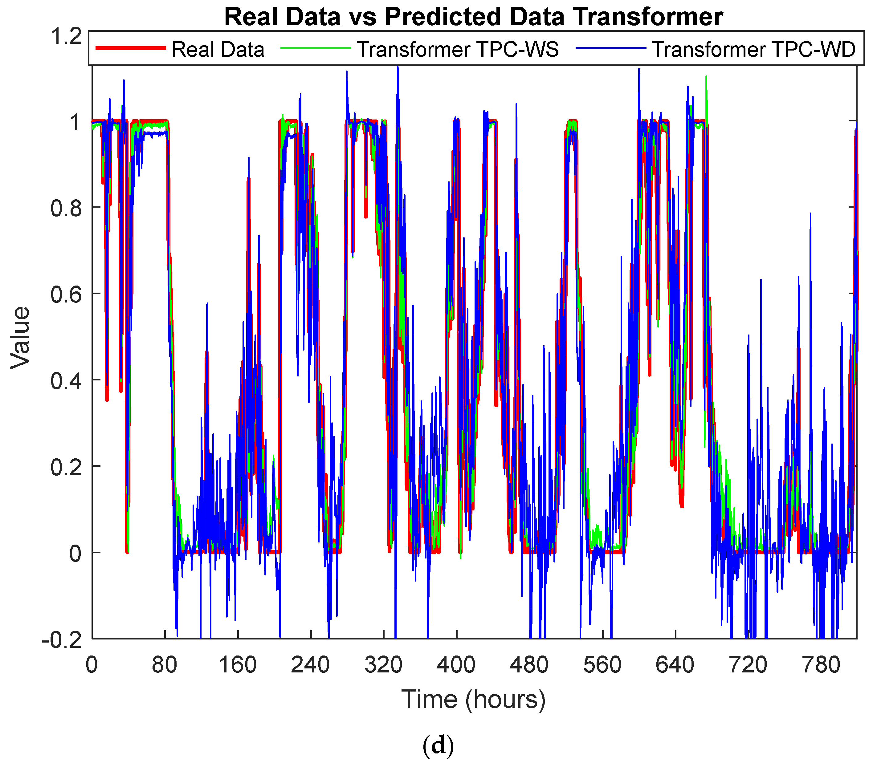
In Figure 7, the actual and predicted powers obtained for the machine learning methodologies are presented. The real data are shown in red, the predictions made with configuration 1 in green, and the predictions made with configuration 2 in blue. The input features in configuration 1 are the theoretical power curve (TPC) and the wind direction (WD). In configuration 2, the wind velocity (WS) is used instead of the wind direction.
The detailed analysis of the four graphs of Figure 7 convincingly reveals that, irrespective of the specific context, configuration 1 (TPC-WS) emerges as the best prediction method over configuration 2 (TPC-WD).
The superiority of configuration 1 lies in its ability to capture the essential dynamics of wind by incorporating wind speed as a key predictive variable. This feature provides a model with a deeper and more accurate understanding of wind patterns, thereby enabling a more precise prediction of the power that will be generated by wind turbines under different atmospheric conditions.
In contrast, configuration 2, which relies solely on the wind direction angle, exhibits lower predictive efficacy compared to its counterpart. While the wind direction angle can provide valuable information about the wind flow orientation, its exclusive use as a predictive variable is proven insufficient to capture the inherent complexity of fluctuations in wind speed, which directly influence the power generated by wind turbines.
The results of the optimal configuration of each deep learning architecture are presented in Figure 8 in order to facilitate a more comprehensive comparison between the methods. In this figure, it is possible to observe that the CNN and transformers models are the models that best fit the target signal, and the GRU model is the worst.
To confirm the better performance of the first configuration, the MAE, RMSE, and WMAPE have been calculated (Table 4).
The set of histograms in Figure 9 shows the error distribution with the four prediction methodologies. The histograms reveal a consistent trend indicating that the CNN and the transformer models outperform the other techniques. Surprisingly, although the GRU model has a lower RMSE, the histogram indicates that errors with larger values are more frequent than with the CNN and transformer models.
The histograms show the frequency distribution of the errors associated with each prediction method. The GRU model exhibits wider error distributions compared to the other methodologies, indicating a lower degree of accuracy and precision of its predictions. In contrast, the CNN and transformer models demonstrate narrower and more acute error distributions, indicative of their superior capability in identifying and adapting to the underlying data patterns and dynamics. This is further evidenced by the concentrated peaks near the zero-error mark, emphasizing the models’ tendency to yield predictions that are closely aligned with the actual values, with a low frequency of substantial errors.
Moreover, the tails of the error histograms of the CNN and transformer models are smaller compared to the GRU model, pointing to a reduced likelihood of extreme deviations and outliers in their predictions. Such characteristics are important for applications where predictability is paramount and the costs of inaccuracies are high.
A series of reflections can be deduced from these results. On the one hand, the technical efficiency of each predictive model is evident, but the results also provide ideas about their practical usefulness. Comparative error analysis suggests that, while GRU models may be beneficial for datasets without complex dependencies, CNN and transformer models are better suited for more complex data sets with more intricate patterns. Exploring these error patterns provides a path for future research which aims to further refine these models, possibly leading to the development of hybrid approaches that leverage the different strengths of each technique to achieve better performance.
6.2. Computational Efficiency and Energy Consumption
In this section, the computational efficiency and implementation feasibility of the predictive models are analyzed. By measuring the predictions per second and the total number of parameters required for each model, a comprehensive assessment is provided for the two tested computing platforms: a conventional computer and a Raspberry Pi 3.
This analysis shows the computational speed and scalability of each model, highlighting their adaptability to resource-constrained environments. Evaluating their performance on both platforms aims to elucidate the practical implications of deploying these models in real-world scenarios, especially where computational resources are limited. These results allow researchers and practitioners to select the most suitable intelligent forecasting model based on its computational efficiency and implementation feasibility.
In Table 5, a comparative analysis of the predictions per second and total number of parameters for both the computer and the Raspberry Pi with the different ML models is presented. The results correspond to configuration 1, with the inputs ‘theoretical power curve (KWh)’ and ‘wind speed (m/s)’. These values correspond to the average iterative execution rate of each method over a one-hour period, as explained in Section 5.3.2. This particular configuration was selected due to our results indicating its superior efficacy in power forecasting (Table 4).
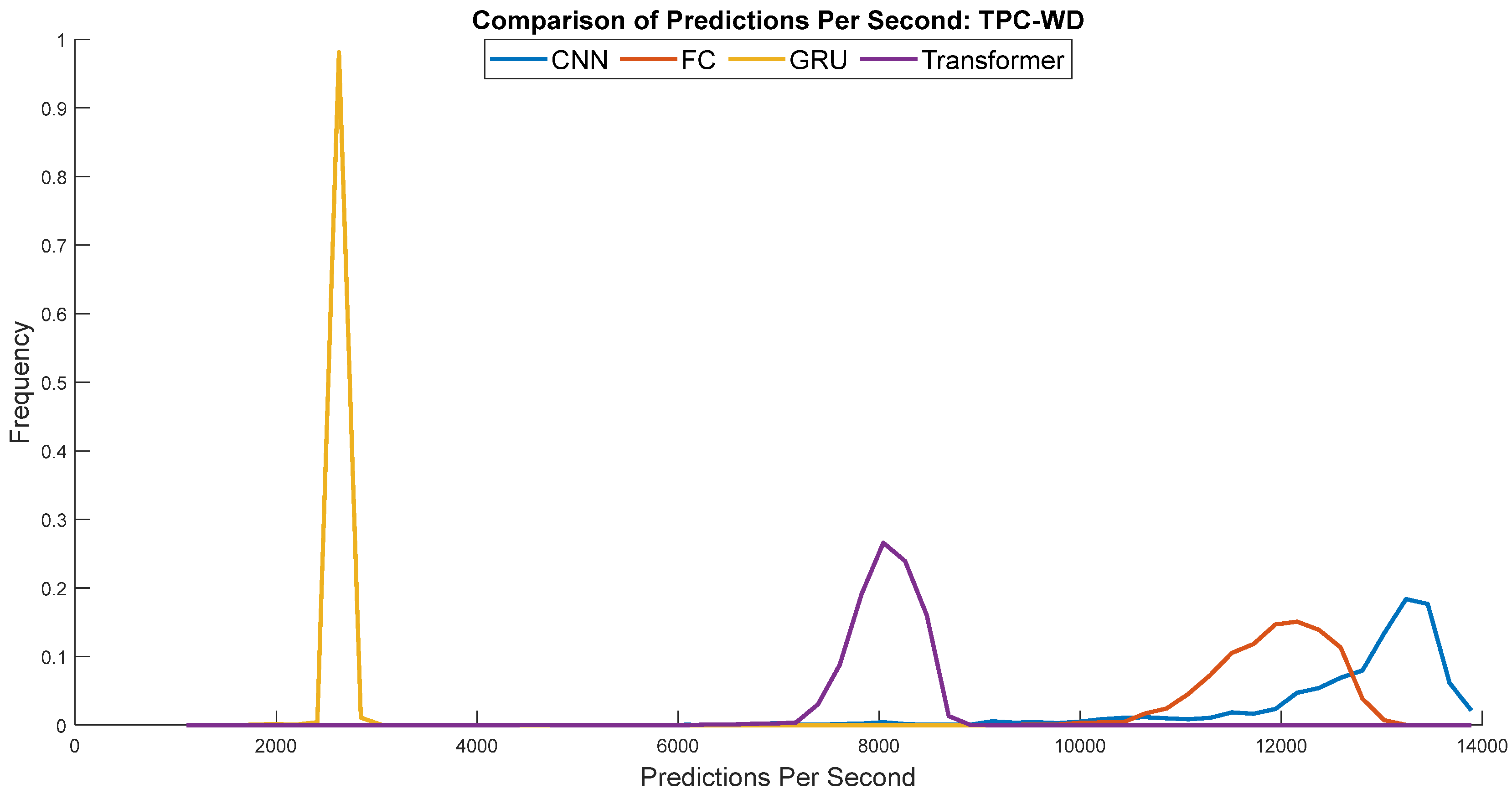
As the number of predictions per second varies during the one-hour experiment, Figure 10 and Figure 11 present the prediction speeds of the different methodologies. This detailed analysis highlights not only the raw computational power but also the real-world applicability of these methods for real-time data processing. Despite occasional drops in prediction speed, the slowest speed observed was 450 predictions per second with the least favorable scenario (GRU architecture on Raspberry Pi), which means one prediction every two milliseconds, a value that is negligible for a typical 100 ms control cycle, which is typically used in the control of small wind turbines.
In addition, the energy expenditure of each method has been measured during its operation, for configuration 1, which considers the theoretical power curve and the wind speed as inputs. As already mentioned, Intel’s Power Gadget 3.6 was used on the Dell computer to measure the aggregated and real-time energy consumption. On the Raspberry Pi, measurement of the input current on the USB-C port was performed with a MINI KPS-PA430 clamp ammeter, with readings taken at five-minute intervals during the hour of the experiment.
Table 6 shows the current and energy consumption obtained in the tests with both hardware systems. As the measured number of predictions per second is different for each architecture, to make a fair comparison between them, the energy has been divided by the number of predictions. These results are shown in Table 7. In terms of energy, the best model is the CNN model, and the worst model, far from the first, is theGRU model.
These figures reveal notable disparities in prediction performance between the two systems that were evaluated. The Dell Vostro 5410, with more computing power, achieved higher predictions per second compared to the Raspberry Pi 3. However, despite its lower performance, the results of the low-cost device are suitable for use in real applications. The slowest case, 450 predictions per second, makes 1 prediction every two milliseconds, which is more than enough for a 100 ms control cycle, as mentioned. This suggests that, although the computational efficiency may vary between hardware platforms, the predictive models evaluated herein remain viable for practical implementation, particularly in scenarios where resource limitations require the use of cheaper hardware solutions.
6.3. Comparison of Multiple Results
To summarize the main findings of this study, Figure 12 presents a comparative graph of the most relevant metrics for the four ML forecasting techniques and the two platforms, the standard computer and RPI. These results have been normalized to the range [0, 1], where lower values indicate better performance. This figure shows that, although they all have advantages and disadvantages regarding speed and resource use, in terms of energy consumption and prediction speed, the GRU technique lags behind in efficiency. The MAE and WMAPE errors are not very different between the different models, so all of these values in the graph are very similar. In view of these results, if we had to select a model, we would choose the CNN model for its lower consumption, speed, and good precision.
This analysis highlights the complex interaction between the efficiency of computational models and their practical accuracy, offering a general description that allows for selecting the most appropriate model for a given application, in this case renewable energy forecasting systems, in scenarios with different computational constraints.
7. Conclusions and Future Works
In this work, an empirical analysis of various intelligent techniques for predicting the power generated by a wind turbine and the possibilities of their implementation on low-cost hardware platforms has been carried out.
Some of the conclusions derived are, for example, the superiority of the wind speed over the direction as the most relevant attribute in prediction. This has been proven with error metrics that measure forecast accuracy.
Of the ML techniques evaluated for this application, the CNN model provides the highest number of predictions per second and the lowest energy consumption, both on the computer and the Raspberry hardware platforms. At the opposite extreme is the GRU model, which provides the lowest real-time performance and highest power consumption. This can be explained by the number of parameters in this model being significantly greater than in the other models. In the case of the Raspberry, the CNN model is 3.62 times faster than the GRU model and requires 84% less energy.
Another interesting result is that the GRU model provides the lowest MAE and RMSE prediction errors; however, it is not the most accurate model. This fact is confirmed by the error histograms; the frequency of larger errors is higher for GRU. Therefore, this fact indicates that these error metrics are not always the best and that other factors must be considered to compare the prediction capacity of the models.
An important aspect of this study is the effectiveness demonstrated by the Raspberry Pi 3, indicating that it is a viable platform to implement these predictive models. Despite its computational limitations, the Raspberry Pi 3 provides good accuracy. This allows us to propose this type of low-cost platform to make the management of these energy resources accessible to a broader public.
By highlighting these results, we emphasize, on the one hand, the viability of some ML techniques for prediction in the context of wind energy and, on the other, the viability of their practical implementation on low-cost platforms with a performance that allows their use in real-time applications in a more accessible way for different users and at different scales.
As future work, we can highlight the integration of these predictions in the control of wind turbines to improve their operation, and their evaluation in a wind turbine prototype.
Author Contributions
P.A.B.-A.: conceptualization, methodology, software, validation, writing—original draft preparation, writing—review and editing. M.P.-Y.: software, validation, writing—original draft preparation, writing—review and editing. J.E.S.-G.: conceptualization, methodology, formal analysis, supervision, software, writing—original draft preparation, writing—review and editing. M.S.: conceptualization, validation, writing—review and editing, supervision. All authors have read and agreed to the published version of the manuscript.
Funding
This research was partially supported by Spanish MICIU/AEI Project PID2021-123543OB-C21.
Data Availability Statement
Data are available from the authors upon reasonable request.
Conflicts of Interest
The authors declare no conflict of interest.
References
- Chen, B.; Xiong, R.; Li, H.; Sun, Q.; Yang, J. Pathways for sustainable energy transition. J. Clean. Prod. 2019, 228, 1564–1571. [Google Scholar] [CrossRef]
- Fawzy, S.; Osman, A.I.; Doran, J.; Rooney, D.W. Strategies for mitigation of climate change: A review. Environ. Chem. Lett. 2020, 18, 2069–2094. [Google Scholar] [CrossRef]
- Muñoz-Palomeque, E.; Sierra-García, J.E.; Santos, M. Wind turbine maximum power point tracking control based on unsupervised neural networks. J. Comput. Des. Eng. 2023, 10, 108–121. [Google Scholar] [CrossRef]
- Pajpach, M.; Haffner, O.; Kučera, E.; Drahoš, P. Low-cost education kit for teaching basic skills for industry 4.0 using deep-learning in quality control tasks. Electronics 2022, 11, 230. [Google Scholar] [CrossRef]
- Afrasiabi, M.; Mohammadi, M.; Rastegar, M.; Afrasiabi, S. Advanced deep learning approach for probabilistic wind speed forecasting. IEEE Trans. Ind. Inform. 2020, 17, 720–727. [Google Scholar] [CrossRef]
- Ponkumar, G.; Jayaprakash, S.; Kanagarathinam, K. Advanced machine learning techniques for accurate very-short-term wind power forecasting in wind energy systems using historical data analysis. Energies 2023, 16, 5459. [Google Scholar] [CrossRef]
- Sri Preethaa, K.R.; Muthuramalingam, A.; Natarajan, Y.; Wadhwa, G.; Ali, A.A.Y. A Comprehensive Review on Machine Learning Techniques for Forecasting Wind Flow Pattern. Sustainability 2023, 15, 12914. [Google Scholar] [CrossRef]
- Zhang, J.; Yan, J.; Infield, D.; Liu, Y.; Lien, F.S. Short-term forecasting and uncertainty analysis of wind turbine power based on long short-term memory network and Gaussian mixture model. Appl. Energy 2019, 241, 229–244. [Google Scholar] [CrossRef]
- Liu, X.; Lin, Z.; Feng, Z. Short-term offshore wind speed forecast by seasonal ARIMA-A comparison against GRU and LSTM. Energy 2021, 227, 120492. [Google Scholar] [CrossRef]
- Buestán-Andrade, P.A.; Santos, M.; Sierra-García, J.E.; Pazmiño-Piedra, J.P. Comparison of LSTM, GRU and transformer neural network architecture for prediction of wind turbine variables. In Proceedings of the International Conference on Soft Computing Models in Industrial and Environmental Applications, Salamanca, Spain, 5–7 September 2023; Springer Nature: Cham, Switzerland, 2023; pp. 334–343. [Google Scholar]
- Ghimire, D.; Kil, D.; Kim, S.H. A survey on efficient convolutional neural networks and hardware acceleration. Electronics 2022, 11, 945. [Google Scholar] [CrossRef]
- Mohaidat, T.; Khalil, K. A Survey on Neural Network Hardware Accelerators. IEEE Trans. Artif. Intell. 2022, 1, 1–21. [Google Scholar] [CrossRef]
- Novac, P.E.; Boukli Hacene, G.; Pegatoquet, A.; Miramond, B.; Gripon, V. Quantization and deployment of deep neural networks on microcontrollers. Sensors 2021, 21, 2984. [Google Scholar] [CrossRef]
- Khalil, K.; Kumar, A.; Bayoumi, M. Reconfigurable hardware design approach for economic neural network. IEEE Trans. Circuits Syst. II Express Briefs 2022, 69, 5094–5098. [Google Scholar] [CrossRef]
- Zhang, G.; Li, B.; Wu, J.; Wang, R.; Lan, Y.; Sun, L.; Lei, S.; Li, H.; Chen, Y. A low-cost and high-speed hardware implementation of spiking neural network. Neurocomputing 2020, 382, 106–115. [Google Scholar] [CrossRef]
- Nguyen, D.A.; Tran, X.T.; Iacopi, F. A review of algorithms and hardware implementations for spiking neural networks. J. Low Power Electron. Appl. 2021, 11, 23. [Google Scholar] [CrossRef]
- Ju, R.Y.; Lin, T.Y.; Jian, J.H.; Chiang, J.S. Efficient convolutional neural networks on raspberry pi for image classification. J. Real-Time Image Process. 2023, 20, 21. [Google Scholar] [CrossRef]
- Ramli, R.; Azri, M.A.; Aliff, M.; Mohammad, Z. Raspberry pi based driver drowsiness detection system using convolutional neural network (cnn). In Proceedings of the 2022 IEEE 18th International Colloquium on Signal Processing & Applications (CSPA), Selangor, Malaysia, 12 May 2022; IEEE: Piscataway, NJ, USA, 2022; pp. 30–34. [Google Scholar]
- Dürr, O.; Pauchard, Y.; Browarnik, D.; Axthelm, R.; Loeser, M. Deep Learning on a Raspberry Pi for Real Time Face Recognition. Eurographics (Posters) 2015, 11–12. [Google Scholar] [CrossRef]
- Çintaş, E.; Özyer, B.; Şimşek, E. Vision-based moving UAV tracking by another UAV on low-cost hardware and a new ground control station. IEEE Access 2020, 8, 194601–194611. [Google Scholar] [CrossRef]
- Akhtari, S.; Pickhardt, F.; Pau, D.; Di Pietro, A.; Tomarchio, G. Intelligent embedded load detection at the edge on industry 4.0 powertrains applications. In Proceedings of the 2019 IEEE 5th International forum on Research and Technology for Society and Industry (RTSI), Florence, Italy, 9–12 September 2019; IEEE: Piscataway, NJ, USA, 2022; pp. 427–430. [Google Scholar]
- Alongi, F.; Ghielmetti, N.; Pau, D.; Terraneo, F.; Fornaciari, W. Tiny neural networks for environmental predictions: An integrated approach with miosix. In Proceedings of the 2020 IEEE International Conference on Smart Computing (SMARTCOMP), Bologna, Italy, 14–17 September 2020; IEEE: Piscataway, NJ, USA, 2022; pp. 350–355. [Google Scholar]
- Jordan, A.A.; Pegatoquet, A.; Castagnetti, A.; Raybaut, J.; Le Coz, P. Deep learning for eye blink detection implemented at the edge. IEEE Embed. Syst. Lett. 2020, 13, 130–133. [Google Scholar] [CrossRef]
- De Vita, F.; Nocera, G.; Bruneo, D.; Tomaselli, V.; Giacalone, D.; Das, S.K. Quantitative analysis of deep leaf: A plant disease detector on the smart edge. In Proceedings of the 2020 IEEE International Conference on Smart Computing (SMARTCOMP), Bologna, Italy, 14–17 September 2020; IEEE: Piscataway, NJ, USA, 2022; pp. 49–56. [Google Scholar]
- Gu, J.; Wang, Z.; Kuen, J.; Ma, L.; Shahroudy, A.; Shuai, B.; Liu, T.; Wang, X.; Wang, G.; Cai, J.; et al. Recent advances in convolutional neural networks. Pattern Recognit. 2018, 77, 354–377. [Google Scholar] [CrossRef]
- Bhatt, D.; Patel, C.; Talsania, H.; Patel, J.; Vaghela, R.; Pandya, S.; Modi, K.; Ghayvat, H. CNN variants for computer vision: History, architecture, application, challenges and future scope. Electronics 2021, 10, 2470. [Google Scholar] [CrossRef]
- Li, Z.; Zhang, Y.; Abu-Siada, A.; Chen, X.; Li, Z.; Xu, Y.; Zhang, L.; Tong, Y. Fault diagnosis of transformer windings based on decision tree and fully connected neural network. Energies 2021, 14, 1531. [Google Scholar] [CrossRef]
- Li, C.; Tang, G.; Xue, X.; Saeed, A.; Hu, X. Short-term wind speed interval prediction based on ensemble GRU model. IEEE Trans. Sustain. Energy 2019, 11, 1370–1380. [Google Scholar] [CrossRef]
- Ji, L.; Fu, C.; Ju, Z.; Shi, Y.; Wu, S.; Tao, L. Short-Term canyon wind speed prediction based on CNN—GRU transfer learning. Atmosphere 2022, 13, 813. [Google Scholar] [CrossRef]
- Lin, C.B.; Dong, Z.; Kuan, W.K.; Huang, Y.F. A framework for fall detection based on OpenPose skeleton and LSTM/GRU models. Appl. Sci. 2020, 11, 329. [Google Scholar] [CrossRef]
- Mahjoub, S.; Chrifi-Alaoui, L.; Marhic, B.; Delahoche, L. Predicting Energy Consumption Using LSTM, Multi-Layer GRU and Drop-GRU Neural Networks. Sensors 2022, 22, 4062. [Google Scholar] [CrossRef] [PubMed]
- Yang, Z.; Mitra, A.; Liu, W.; Berlowitz, D.; Yu, H. TransformEHR: Transformer-based encoder-decoder generative model to enhance prediction of disease outcomes using electronic health records. Nat. Commun. 2023, 14, 7857. [Google Scholar] [CrossRef]
- Erisen, B. Wind Turbine Scada Dataset. Kaggle. 2018. Available online: https://www.kaggle.com/datasets/berkerisen/wind-turbine-scada-dataset/code (accessed on 3 April 2023).
- Li, L.; Talwalkar, A. Random search and reproducibility for neural architecture search. In Proceedings of the 35th Uncertainty in Artificial Intelligence Conference, Tel Aviv, Israel, 22–25 July 2019; pp. 367–377. [Google Scholar]
- Martikkala, A.; David, J.; Lobov, A.; Lanz, M.; Ituarte, I.F. Trends for low-cost and open-source IoT solutions development for industry 4.0. Procedia Manuf. 2021, 55, 298–305. [Google Scholar] [CrossRef]
- Intel. 2023. Available online: https://www.intel.com/content/www/us/en/developer/articles/training/using-the-intel-power-gadget-30-api-on-windows.html (accessed on 6 April 2024).
Figure 1.
CNN architecture [26].
Figure 1.
CNN architecture [26].

Figure 2.
Fully connected neural network architecture [27].
Figure 2.
Fully connected neural network architecture [27].

Figure 3.
Gated recurrent unit (GRU): (a) reset gate; (b) update gate [30].
Figure 3.
Gated recurrent unit (GRU): (a) reset gate; (b) update gate [30].

Figure 4.
Architecture of the transformer model [10].
Figure 4.
Architecture of the transformer model [10].

Figure 5.
Histograms of the time series of the wind turbine dataset: active power, theoretical power curve, wind speed, and wind direction.
Figure 5.
Histograms of the time series of the wind turbine dataset: active power, theoretical power curve, wind speed, and wind direction.

Figure 6.
Wind speed (a) and wind direction (b) signals used to test the models.

Figure 7.
(a) Real data vs. predicted data comparison with fully connected model. (b) Real data vs. predicted data comparison with CNN model. (c) Real data vs. predicted data comparison with GRU model. (d) Real data vs predicted data comparison with transformers model.
Figure 7.
(a) Real data vs. predicted data comparison with fully connected model. (b) Real data vs. predicted data comparison with CNN model. (c) Real data vs. predicted data comparison with GRU model. (d) Real data vs predicted data comparison with transformers model.


Figure 8.
Real data vs. predicted data comparison of best models.

Figure 9.
Error histogram of the different techniques: (a) FC model. (b) CNN model. (c) GRU model. (d) Transformer model.
Figure 9.
Error histogram of the different techniques: (a) FC model. (b) CNN model. (c) GRU model. (d) Transformer model.


Figure 10.
Histogram of predictions per second of the different techniques for a one-hour experiment with the Dell Vostro 5410 computer.
Figure 10.
Histogram of predictions per second of the different techniques for a one-hour experiment with the Dell Vostro 5410 computer.

Figure 11.
Histogram of predictions per second of the different techniques for a one-hour experiment with the Raspberry Pi 3.
Figure 11.
Histogram of predictions per second of the different techniques for a one-hour experiment with the Raspberry Pi 3.

Figure 12.
Comparative analysis of predictive models’ performance in terms of computational and accuracy metrics.
Figure 12.
Comparative analysis of predictive models’ performance in terms of computational and accuracy metrics.


Table 1.
Comparative analysis of low-cost hardware implementations of machine learning applications.
Table 1.
Comparative analysis of low-cost hardware implementations of machine learning applications.
| Reference | Application | Hardware | Architecture | Accuracy | Real-Time Performance | Energy |
|---|---|---|---|---|---|---|
| This work | Wind Power Forecasting | Raspberry Pi 3 | CNN, Fully Connected, Transformer, GRU | Yes | Yes | Yes |
| Durr, O et al. 2015 [19] | Real Time Face Recognition | Raspberry Pi 3 | CNN | Yes | Yes | No |
| Cintas, E. 2020 [20] | Vision Based Moving UAV Tracking by another UAV | Raspberry Pi 4 | CNN | Yes | No | No |
| S. Akhtari et al. 2019 [21] | Applied load in a power train system monitoring | STM32 | DNN | Yes | No | No |
| F. Alongi et al. 2020 [22] | Weather Forecasting | STM32 | DTNN | Yes | No | No |
| Jordan, A et al. 2020 [23] | Eye blink detection | STM32L451 | CNN | Yes | Yes | Yes |
| F. de Vita et al. 2020 [24] | Diseases in coffee plants detection | STM32 | Q-CNN | Yes | Yes | Yes |
| Ju et al. 2023 [17] | Image classification | Raspberry | HarDNet, ThreshNet, ShuffleNet, MobileNetV1, GhostNet, EfficientNet | Yes | Yes | No |
Table 2.
Main parameters of the histograms of the time series of the wind turbine dataset.
| Parameter | LV ActivePower (kW) | Wind Speed (m/s) | Theoretical Power Curve (KWh) | Wind Direction (°) |
|---|---|---|---|---|
| Mean | 1307.68 | 7.56 | 1492.17 | 123.69 |
| Standard Deviation | 1312.46 | 4.23 | 1368.02 | 93.44 |
| Min | −2.47 | 0.00 | 0.00 | 0.00 |
| 25% Quartile | 50.68 | 4.20 | 161.33 | 49.31 |
| 50% Quartile | 825.84 | 7.10 | 1063.78 | 73.71 |
| 75% Quartile | 2482.51 | 10.30 | 2964.97 | 201.70 |
| Max | 3618.73 | 25.21 | 3600.00 | 360.00 |
Table 3.
Hyperparameters of each ML method obtained with random search.
| Input Features | FC | CNN | GRU | Transformers |
|---|---|---|---|---|
| Theoretical power curve and wind speed CONF 1 | Window: 20 Num_layers: 3 Units: 128 Activation: relu Dropout rate 0.1 | Window: 20 Num_layers: 2 Filters 128 Core_size: 3 Activation: leaky_relu Pool_size: 3 Dropout rate 0.1 | Window: 60 Num_layers: 2 Filters: 128 Dropout_rate: 0.1 | Window: 20 Num_layers: 2 Num_heads: 3 Ff_dim: 32 Key_dim: 3 |
| Theoretical power curve and wind direction CONF 2 | Window: 20 Num_layers: 3 Units: 128 Activation: relu Dropout rate 0.1 | Window: 20 Num_layers: 2 Filters 128 Core_size: 3 Activation: leaky_relu Pool_size: 3 Dropout rate 0.1 | Window: 60 Num_layers: 2 Filters: 32 Dropout_rate: 0.1 | Window: 20 Num_layers: 2 Num_heads: 8 Ff_dim: 128 Key_dim: 3 |
Table 4.
Comparison of prediction errors.
| Theoretical Power Curve and Wind Speed (Configuration 1) | Theoretical Power Curve and Wind Direction (Configuration 2) | |||||||
|---|---|---|---|---|---|---|---|---|
| Architecture | RMSE | MAE | WMAPE | RMSE | MAE | WMAPE | ||
| Fully Connected | 0.0581 | 0.033 | 0.9797 | 0.0854 | 0.0736 | 0.052 | 0.9674 | 0.1344 |
| CNN | 0.0596 | 0.033 | 0.9786 | 0.0852 | 0.0807 | 0.0544 | 0.9608 | 0.1432 |
| GRU | 0.0581 | 0.0326 | 0.9794 | 0.0853 | 0.0703 | 0.0497 | 0.97 | 0.13 |
| Transformer | 0.0691 | 0.0405 | 0.9713 | 0.1047 | 0.1313 | 0.0885 | 0.8962 | 0.2289 |
Table 5.
Hardware performance comparison for the ML forecasting techniques with inputs TPC and WS.
| Architecture | (Computer) | (Raspberry Pi 3) | Total Parameters |
|---|---|---|---|
| Fully Connected | 11,895 | 2093 | 36,097 |
| CNN | 12,698 | 2971 | 116,353 |
| GRU | 2640 | 820 | 150,273 |
| Transformer | 8057 | 1997 | 558 |
Table 6.
Comparison of accumulated energy for medium- and low-cost hardware devices.
| Architecture | ||||
|---|---|---|---|---|
| Fully Connected | 6.606 | 11.362 | 0.207 | 1.035 |
| CNN | 6.740 | 11.593 | 0.198 | 0.988 |
| GRU | 10,114 | 17.396 | 0.357 | 1.785 |
| Transformer | 6.320 | 10.870 | 0.227 | 1.135 |
Table 7.
Comparison of accumulated relative energy for medium- and low-cost hardware.
| Architecture | ||||
| Fully Connected | 555.36 | 955.19 | 98.901 | 494.505 |
| CNN | 530.79 | 912.98 | 66.644 | 332.548 |
| GRU | 3831.10 | 6589.41 | 435.366 | 2177.83 |
| Transformer | 784.41 | 1349.13 | 113.671 | 568.353 |
Disclaimer/Publisher’s Note: The statements, opinions and data contained in all publications are solely those of the individual author(s) and contributor(s) and not of MDPI and/or the editor(s). MDPI and/or the editor(s) disclaim responsibility for any injury to people or property resulting from any ideas, methods, instructions or products referred to in the content. |
© 2024 by the authors. Licensee MDPI, Basel, Switzerland. This article is an open access article distributed under the terms and conditions of the Creative Commons Attribution (CC BY) license (https://creativecommons.org/licenses/by/4.0/).
Share and Cite
MDPI and ACS Style
Buestán-Andrade, P.A.; Peñacoba-Yagüe, M.; Sierra-García, J.E.; Santos, M. Wind Power Forecasting with Machine Learning Algorithms in Low-Cost Devices. Electronics 2024, 13, 1541. https://doi.org/10.3390/electronics13081541
AMA Style
Buestán-Andrade PA, Peñacoba-Yagüe M, Sierra-García JE, Santos M. Wind Power Forecasting with Machine Learning Algorithms in Low-Cost Devices. Electronics. 2024; 13(8):1541. https://doi.org/10.3390/electronics13081541
Chicago/Turabian StyleBuestán-Andrade, Pablo Andrés, Mario Peñacoba-Yagüe, Jesus Enrique Sierra-García, and Matilde Santos. 2024. "Wind Power Forecasting with Machine Learning Algorithms in Low-Cost Devices" Electronics 13, no. 8: 1541. https://doi.org/10.3390/electronics13081541
Note that from the first issue of 2016, this journal uses article numbers instead of page numbers. See further details here.