
Control Parameters Design of Spraying Robots Based on Dynamic Feedforward

School of Mechanical Science and Engineering, Huazhong University of Science and Technology, Wuhan 430074, China
*
Author to whom correspondence should be addressed.
Electronics 2024, 13(8), 1583; https://doi.org/10.3390/electronics13081583
Submission received: 23 March 2024
/
Revised: 18 April 2024
/
Accepted: 19 April 2024
/
Published: 21 April 2024
(This article belongs to the Special Issue The Application of Control Systems in Robots)
Abstract
:The positioning and velocity accuracy of spraying robots determine the quality of the coating, and the influence of the robotic dynamic characteristics on control precision is significant. This paper presents a method of linearizing dynamic characteristics into feedforward coefficients and designs a dual-loop control system consisting of an inner velocity loop and an outer position loop. The system is divided into three sections: a cascaded section, a feedback section, and a feedforward section. The cascaded section eliminates the nonlinear characteristics of the system; the feedback section ensures the stability of the system; the feedforward section compensates for the internal errors of the system. The main innovation of this paper lies in proposing an offline parameter tuning method, which avoids online parameter adjustments and significantly enhances the real-time performance of the control system. Additionally, this method does not require specific physical information of the system, thus avoiding the cumbersome process of parameter adjustment. The experimental results demonstrate that when facing different high-speed trajectories, the proposed control system exhibits a significant improvement in control accuracy compared to other advanced control schemes.
1. Introduction
Spraying robots are widely used automation devices in the industrial sector [1,2]. They are capable of performing coating tasks on surfaces of automobiles, aircraft, spacecraft, and other structures with high speed and precision [3,4,5,6]. In comparison to manual spraying, these robots possess faster operation speeds and higher stability, while also being adaptable to various intricate shapes. Therefore, they can significantly enhance production efficiency and product quality [7].
The quality of surface coatings directly affects product performance. Maintaining stable speed control is crucial for achieving high-quality coatings. When the spraying speed of a spraying robot is too slow, it leads to an insufficient curing of the coating, causing bubbles and wrinkles. Conversely, an excessive spraying speed makes the coating’s quality fragile. Therefore, spraying robots need to possess not only high-precision position control capabilities but also ensure that speed control is highly accurate and stable. High-DOF robotic arms can cover a wide range of workspaces, adapt to various scales and sizes of working environments, and achieve precise motion control. Therefore, high-DOF robotic arms are widely applied in the field of spraying robots [8,9,10].
Proportional-integral-derivative (PID) control is the most common controller in the field of industrial robots. However, for robot systems with significant gravity effects such as spraying robots, PID control can lead to the presence of steady-state errors [11]. According to Arimoto S et al., by selecting appropriate proportional-integral-derivative gains, it is possible to achieve asymptotic stable set-point control within a local range [12]. To overcome the influence of steady-state errors as much as possible, scholars have proposed control schemes such as nonlinear PID [13], fuzzy PID [14], and neural network PID [15]. However, the aforementioned control strategies have not fully utilized the dynamic model, making it difficult to meet the demand for stable speed control. The spraying robot system is highly complex, exhibiting characteristics of strong nonlinearity, time-varying characteristics, and strong coupling. Particularly during high-speed motion, the robot’s inertia undergoes significant changes, leading to a pronounced increase in nonlinear effects. As a result, these control strategies are prone to causing control instability and system oscillations [16].
Control methods based on the robot’s dynamic model are widely regarded as the most effective approach to enhancing robot dynamic characteristics and trajectory tracking accuracy. Currently, scholars have proposed various advanced control schemes that integrate dynamic characteristics of industrial robots [17,18,19,20,21]. However, these strategies still face challenges in spraying robots due to computational efficiency limitations. Currently, incorporating dynamic feedforward into closed-loop feedback control schemes remains the mainstream approach in the industrial sector [22,23]. In this control scheme, the feedforward component is utilized to compensate for dynamic characteristics, while the feedback component is further finely adjusted based on control errors to maintain system stability. In related research, Santibanez et al. demonstrated that appropriate gains can ensure global asymptotic stability [24]. Caccavale et al. conducted studies on dynamic parameter identification and feedforward control for robots [25]. Abe et al. conducted research on feedforward control for flexible dual-arm robots [26].
Currently, research on spraying robots primarily focuses on two aspects: firstly, how to incorporate dynamic models, and secondly, addressing the uncertainty of dynamic parameters. Regarding the first aspect, Zhang Binbin et al. proposed a method for achieving the precise dynamic feedforward control of spraying robots in large workspaces and under time-varying dynamic conditions [27]. Yu Chen et al. proposed a nonlinear adaptive robust control scheme based on desired trajectory [28]. Zilin Liu et al. proposed a strategy for tuning control parameters for spraying robots based on small noise excitation [29]. The aforementioned strategies all require physical information of the robot system (such as joint masses, centers of mass, and moments of inertia), and the process of tuning control system parameters is both intricate and time consuming.
Regarding the second aspect, Yi-Liang Yeh proposed a robust noise-free linear control scheme for robot manipulator [30]. Han Zhao et al. introduced an adaptive robust constrained control scheme for bicycle robots under uncertainties [31]. Liu et al. established a friction model for spraying robots and devised an outer-loop adaptive control scheme [32]. Zhong Wang et al. proposed an active disturbance rejection controller based on an extended state observer and designed a feedforward control strategy with deviation compensation [33]. Xin Cheng et al. proposed a dynamic feedforward-based active disturbance rejection control strategy to overcome uncertainties and disturbances [34]. However, these control methods all require real-time parameter adjustments within the control system, which compromises control performance.
To overcome the above challenges, this paper proposes a method to linearize the dynamic model into feedforward coefficients and provides a technique to adjust various control parameters of the system. The main contributions of this paper can be summarized as follows:
- This control strategy translates the dynamic model into feedforward coefficients within the control system, effectively transforming complex dynamic characteristics into a parameter tuning problem, thus improving the response speed of the control system.
- The control parameters of this strategy can be roughly determined, reducing the laborious debugging work typically required by engineers.
- When determining the feedforward coefficients, this control strategy only requires current measurements, eliminating the need for various detailed system information such as dynamic parameters and gearbox damping ratios.
The structure of this paper is as follows: Section 2 deduces the linearization method for robot dynamics. Section 3 presents the design methodology of the control system. Section 4 describes the approach for determining the control coefficients of the system. Section 5 provides a detailed presentation of the experimental results. Section 6 presents the discussion and Section 7 presents the conclusion.
2. Dynamic Linearization
In industrial applications, n-DOF manipulators are commonly used as the platforms for spraying robots. Therefore, the focus of this paper is primarily on such manipulators. The position of robot joint is determined by a series of preceding joint rotation angles [35], where . Therefore, the center of mass positions for each joint can be expressed as functions of , and the potential energy of the system, denoted as P, can be represented as (1):
where is the component of along the axis opposite to gravity, represents the mass of joint . The total kinetic energy K of the system is composed of three parts: the translational kinetic energy of each joint K1, the rotational kinetic energy of each joint K2, and the rotational kinetic energy of each drive motor K3. The center of mass velocity for each joint can be expressed as (2):
The total kinetic energy K of the system can be expressed as
where is the inertia tensor matrix of joint . represents the angular velocity of joint , which is determined by and , and can be solved using the Newton–Euler method. denotes the rotational inertia of the drive motor for joint . k stands for the damping ratio.
By substituting (1) and (3) into the Lagrange’s equation, where , we can derive the driving torques for each motor :
Since is a function of both and , its derivative with respect to time t can be divided into two parts, as shown in (5):
Substituting Equation (5) into Equation (4), we obtain
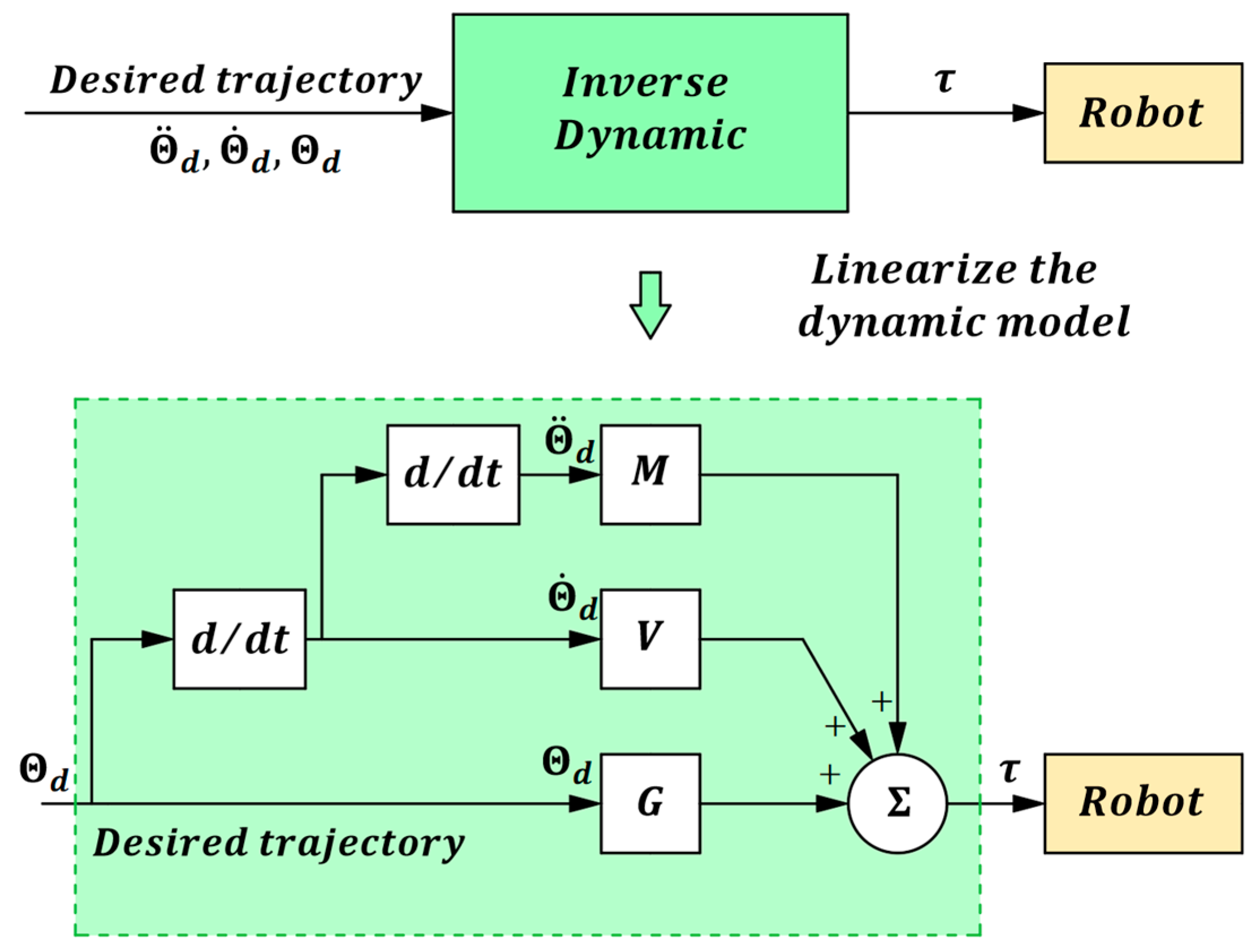
We linearize Equation (6) as shown in Equation (7):
where and are the generalized inverses of and , respectively, and M represents the acceleration gain diagonal matrix, and . V is the velocity gain diagonal matrix, and . G stands for the position gain diagonal matrix, and . Through this linearization approach, we can transform dynamical models with nonlinear and strongly coupled characteristics into feedforward coefficients, thereby enhancing the system’s response speed. The process of linearizing the robot’s dynamic model is illustrated in Figure 1.
3. Control System Design
The control system is divided into three parts: a cascade section, a feedback section, and a feedforward section. The cascade section not only enhances the system’s disturbance rejection capability but also eliminates the system’s nonlinear characteristics. The feedback section ensures the closed-loop stability of the system. The feedforward section consists of two parts: internal error compensation and the linearized dynamic feedforward.
3.1. Cascade Section
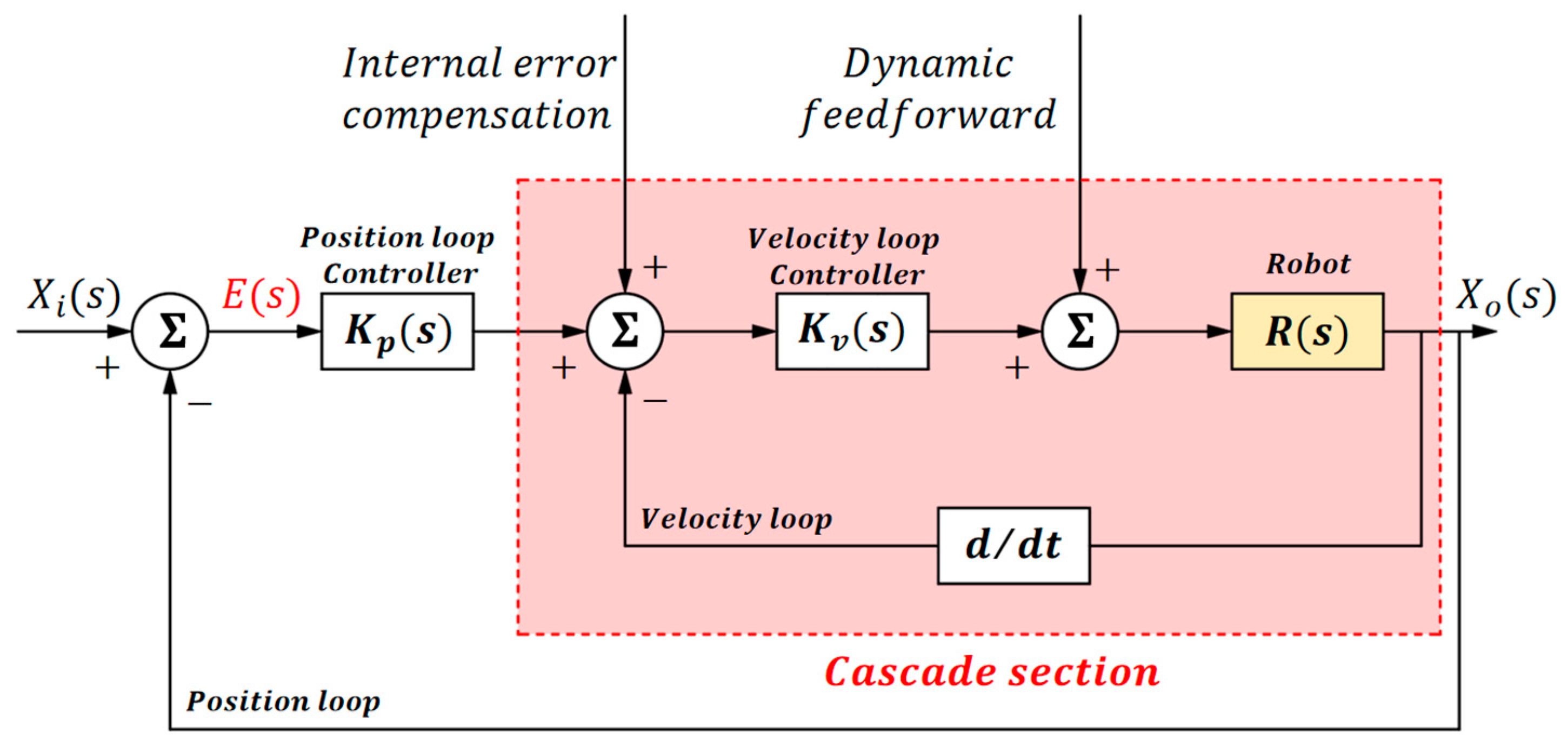
The control loop consists of an outer position loop and an inner velocity loop. As shown in Figure 2, the inner velocity loop corresponds to the cascade section. When the robot is affected by disturbances, the disturbances are first adjusted by the inner velocity loop and then further adjusted by the outer position loop. This further enhances the control quality of the system.
Furthermore, the cascade section can eliminate the nonlinear characteristics of the system. We can denote the transfer function of the robot as R(s). Choosing a proportional controller for the velocity loop, we have . The transfer function of the cascade section is given by (8).
When the velocity gain coefficient is much greater than 1, the transfer function of the cascade section can be simplified to an integral element: . Through the cascade section, we can eliminate the influence of R(s) with complex nonlinear characteristics.
3.2. Feedback Section
Based on the analysis in the cascade section, we can equivalently represent the inner velocity loop as an integral element. The equivalent closed-loop system is shown in Figure 3. We set the position loop controller as a proportional-integral controller, where , with T as the integral time constant. Then, the transfer function G(s) of the entire closed-loop system is as shown in (9).
In the above equation, represents the undamped natural frequency of the system, and is the damping ratio of the system. It can be observed that the robot control system is a second-order system. In order to achieve the best possible dynamic response of the control system, it is common in engineering to set the damping ratio of a second-order system to be . This results in (10):
When the damping ratio is fixed at , . In this case, the transfer function G(s) of the closed-loop system is as shown in (11):
Due to the fact that the feedforward section does not affect the closed-loop stability of the system, we can analyze the overall system’s stability based on the closed-loop transfer function in (11). According to the Routh Criterion, as long as , the system can be guaranteed to be stable. And as shown in Figure 4, when different values of are selected, the root locus of the system consistently lies on the left-hand side of the complex plane, confirming the system’s stability.
3.3. Feedforward Section
According to the Routh Criterion, as long as , the system can be guaranteed to be stable. And as shown in Figure 4, when different values of are selected, the root locus of the system consistently lies on the left-hand side of the complex plane, confirming the system’s stability. The feedforward section consists of two components: internal error compensation and linearized dynamic feedforward. In a control system, our objective is to make the system’s desired signal as closely equal to the output signal as possible in the absence of external disturbances, i.e., . To achieve this goal, we introduce an internal error compensation block to ensure that the system’s internal error . This can be expressed as (12):
4. Determination of Control System Parameters
Since the feedforward section does not affect the system’s stability, we can independently design the system’s feedforward and feedback coefficients. The control precision of a control system is primarily determined by the dynamic model. Therefore, the emphasis of this section is on determining the feedforward coefficients, and there is no need to spend too much time on determining the feedback coefficients.
4.1. Determination of Feedback Coefficients
Feedback coefficients include , , and T. According to the analysis in Section 3, it is known that the position loop coefficient is determined by the integral time T, and the velocity loop coefficient needs to be much greater than 1. They satisfy the relationship of and . Therefore, it is only necessary to determine the integral time T and velocity loop coefficient for each joint.
For , as the velocity inner loop serves only for preliminary adjustment, we can initially set the velocity loop proportional coefficients for each joint roughly, and then fine-tune the control system with the outer position loop for precision adjustment. In this paper, the proportional coefficients for the velocity loop of each joint are set to 100.
For , the integral time for each joint can be determined using the Ziegler–Nichols method [36]. We place the robot’s closed-loop system in an unloaded state, record the period of current oscillations, and initially set the integral time constant T to this oscillation period. Subsequently, we iteratively adjust the time constant T repeatedly to achieve optimal performance. The feedback coefficients for each joint are shown in Table 1.
4.2. Determination of Dynamic Feedforward Coefficients
Feedforward coefficients include , , and . For different task trajectories, it is necessary to identify different feedforward coefficients. The process of determining the feedforward parameters for each joint is illustrated in Figure 6.
We pre-run the task trajectory using a PID control scheme, where the proportional coefficient and integral time constant T in the PID strategy can be consistent with the previously determined feedback coefficients. We record the current values of each drive motor corresponding to the task trajectory, and then filter the current to remove noise interference as much as possible. The filtered current values are denoted as . These current values can be approximated as the actual current required by each motor drive.
To make the linearized dynamic feedforward as closely as possible consistent with the real robot dynamics, we aim for the current values provided by the dynamic feedforward in the control system to be as equal as possible to the actual current values required by the robot’s individual drive motors. The approach used in this paper is independent joint control, where the dynamic parameters of each joint are identified separately. From (7), it can be seen that the feedforward coefficients for each joint, denoted as , , , determine the current values provided by the dynamic feedforward, taking joint i as an example, as illustrated in (13):
To make the dynamic feedforward as closely aligned with the real current values as possible, we can adjust the feedforward coefficients , , to ensure that closely matches . The process of adjusting these parameters can be formulated as an optimization problem. The optimization objective is as depicted in (14), and is further illustrated in Figure 7 where k represents the number of points for collecting current, and the design variables are , , .
4.3. Solving the Optimization Problem
This paper employs the particle swarm optimization (PSO) algorithm to solve the optimization problem. PSO is an optimization algorithm based on swarm intelligence, where candidate solutions are treated as particles. Each particle continuously adjusts its position in the solution space based on its individual best and the global best, aiming to find the optimal solution. This algorithm is capable of rapidly searching for an approximate optimal solution to the objective function.
The PSO algorithm has advantages such as simplicity and ease of implementation. Compared to traditional optimization algorithms, it does not require gradient information of the objective function; compared to modern intelligent algorithms such as genetic algorithms, it does not require complex operations like crossover and mutation. For unconstrained optimization problems with a large search space like those in this paper, using the PSO algorithm enables a parallel search, facilitating the rapid and efficient discovery of the optimal solution.
The feedforward coefficients, namely , , and are treated as particles. Each particle i possesses position and velocity attributes, and the corresponding fitness function is denoted as , where position represents the solution to the problem, and represents the direction of solution updating. Particles update themselves by tracking two positions: one is the best position that particle i has experienced so far, and the other is the best position that the particles in the population have collectively achieved. The particles update their velocity and position based on Equations (15) and (16):
where are all weighting coefficients, while are random values between . represents the particle’s update in the direction of individual best, and represents the particle’s update in the direction of global best.
This paper utilizes the PSO algorithm, setting the number of iterations s to 200. Throughout the entire iteration process, the position of the particle with the minimum fitness is selected as the feedforward coefficient. The feedforward coefficients identified for the two task trajectories in this paper are shown in Table 2 and Table 3. When the task trajectory is high-speed back-and-forth linear movements, the current fitting results for joints 1 to 4 are shown in Figure 8. Using this approach, we simplify the complex dynamic model into an adjustment process for feedforward parameters. Importantly, this process does not require knowledge of the physical characteristics of each robot joint (such as mass, center of mass, moment of inertia) or details like friction coefficients, gearbox damping ratios, and other information. Additionally, because we can calculate the dynamic parameters offline, avoiding real-time computations required by other methods, it enhances the universality of our approach.
5. Experiment and Result
5.1. The Experimental Platform and Simulation
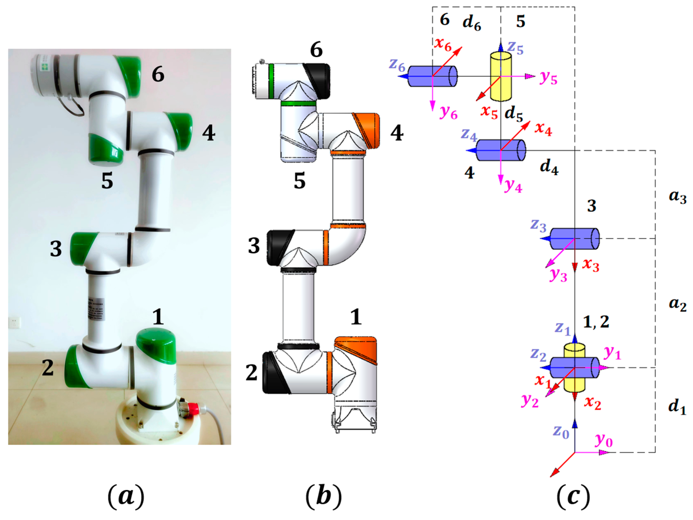
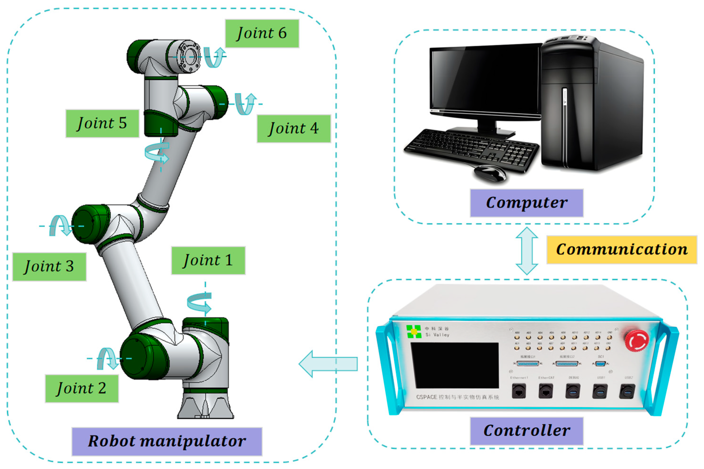
This paper conducts research on a six-DOF robot developed by a Chinese company, Si Valley [37]. Its physical structure and coordinate system are illustrated in Figure 9. On the left side of Figure 9 is the actual robotic arm, in the middle is the SolidWorks model of the robotic arm, and on the right side is the coordinate system of the robotic arm. Its D-H parameters are presented in Table 4. The specific parameters of the robot are shown in [33]. The experimental platform is shown in Figure 10. The controller adopts its self-developed cSPACE rapid control prototype development system. The software is developed based on ARM Cortex-A and Matlab/Simulink 2023a.
We develop our control methods in the Simulink environment, transferring the programs to the controller via the computer, where the controller issues commands to the robot and communicates with the host computer. To verify that our method can remain stable under external disturbances, we conducted simulations in Simulink by applying noise signals to each joint. It can be observed that the robot still maintains high-precision tracking performance from Figure 11.
5.2. The Task Trajectory Information of Physical Experiments in Real World
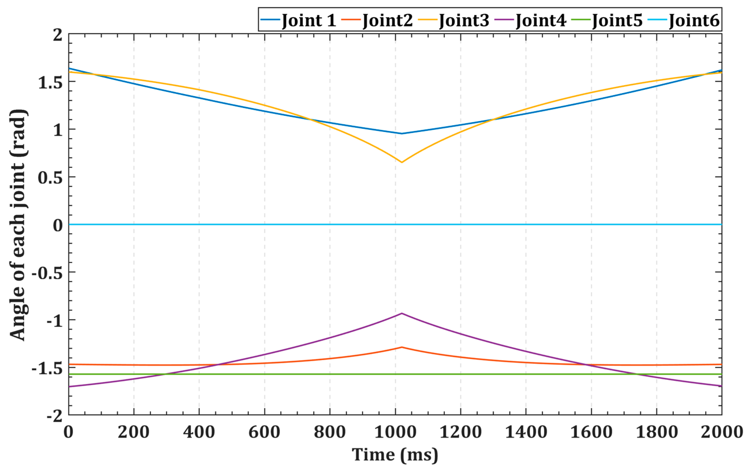
To validate the effectiveness of our control method in real-world scenarios, experiments were conducted in a physical environment. This paper conducted tests on two types of task trajectories in the real world: a high-speed back-and-forth linear trajectory and a high-speed circular trajectory. Both of these trajectories took only 2 s to complete. These two trajectories are respectively shown in Figure 12 and Figure 13. It can be seen that only the changes in joints 1–4 are significant, so we mainly focus on controlling the first four joints.
For the aforementioned task trajectories, we adopted three different control strategies. The first one is the PID control strategy, the second is the method proposed in this paper, and the third is the current advanced real-time robust control strategy. Real-time robust control is a control method specifically proposed for the uncertain parameters of the controlled object described in this paper, so we compared it with the method proposed in this paper. To ensure a fair comparison, we set the parameters in the PID strategy to be the same as the feedback parameters in this paper.
5.3. The Back-and-Forth Linear Trajectory
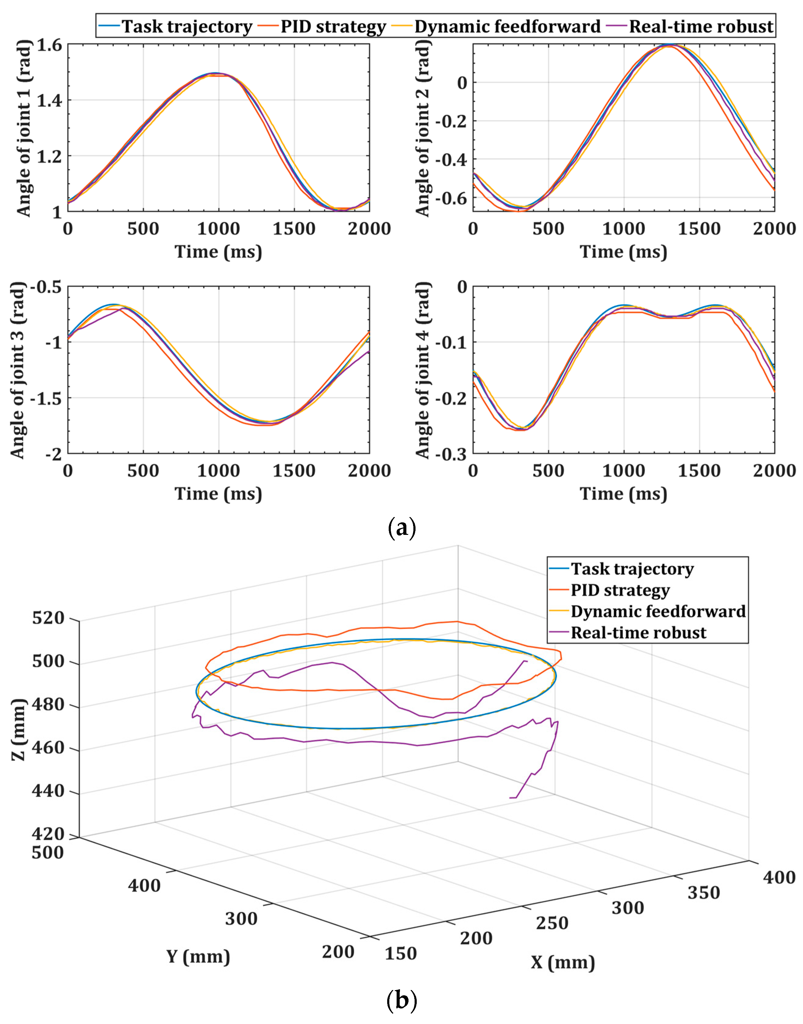
We employed three different control strategies, namely, a PID strategy, a dynamic feedforward strategy, and a real-time robust control strategy, to track the high-speed back-and-forth trajectory. Figure 14 illustrates the control performance of these three methods in both joint space and three-dimensional space, respectively. Figure 15 shows the position and velocity errors of the end effector under the three control strategies, respectively. Table 5 shows the joint tracking errors for each control method. Table 6 provides a comparison of the trajectory tracking performance differences between these three control strategies.
5.4. The Circular Trajectory
We employed three different control strategies, namely, a PID strategy, a dynamic feedforward strategy, and a real-time robust control strategy, to track the high-speed circular trajectory. Figure 16 illustrates the control performance of these three methods in both joint space and three-dimensional space. Figure 17 shows the position and velocity errors of the end effector under the three control strategies. Table 7 shows the joint tracking errors for each control method. Table 8 provides a comparison of the trajectory tracking performance differences between these three control strategies.
6. Discussion
We employed three different control strategies, namely, a PID strategy, a dynamic feedforward strategy, and a real-time robust control strategy. From Table 5 and Table 7, it can be seen that our method outperforms the other two methods in terms of joint tracking performance. To analyze the positional and velocity accuracies of these three methods in Cartesian space, we have compiled Table 6 and Table 8 into Table 9 and Table 10.
In terms of positional accuracy, for the linear trajectory, the average position error of the dynamic feedforward strategy is only 5.90 mm, which represents an increase in accuracy of 62.5% compared to the PID strategy used for identification. For the circular trajectory, the average position error of the dynamic feedforward strategy is 2.67 mm, which represents an increase in accuracy of 92.2% compared to the PID strategy. This indicates that the integration of dynamic feedforward enables the system to respond proactively, reducing the burden on the feedback loop, and thereby significantly enhancing the positional tracking precision.
In terms of velocity accuracy, for the linear trajectories, the average error of the dynamic feedforward strategy is only 0.003 mm/s, representing an increase in accuracy of 88.9% compared to the PID strategy. For the circular trajectory, the average position error of the dynamic feedforward strategy is 0.001 mm/s, indicating an improvement in accuracy of 91.6% compared to the PID strategy. This indicates that the dual-loop control system employed in this paper can effectively adjust velocity errors, thereby ensuring velocity stability.
Based on the above experiments, it is evident that when applying different high-speed reference trajectories, the use of a dynamic feedforward control strategy results in significantly lower errors across all aspects compared to employing the pure PID control strategy. This outcome strongly validates the effectiveness of our approach.
7. Conclusions
The control precision of spraying robots determines the quality of the coating, with the dynamic characteristics significantly influencing the control performance of the robot. This paper proposes a control strategy based on a dynamic feedforward strategy for spraying robots and provides a method for determining various control parameters within the system. We have validated our method through both simulation and physical experiments. Experimental results demonstrate that this control strategy achieves excellent tracking performance for various high-speed reference trajectories, with a significantly higher tracking accuracy compared to control strategies that do not employ dynamic feedforward. The main advantages of our approach in this paper are as follows:
- The control strategy proposed in this paper converts complex dynamic models into feedforward coefficients for the control system, thus enhancing the real-time performance of the control system.
- This paper presents a method for determining control parameters, avoiding the time-consuming and labor-intensive process of tuning.
- The control strategy proposed in this paper only requires measuring current to determine the feedforward coefficients, without the need for any additional information.
However, our method still has the following limitations:
- The industrial system needs to have the capability to measure control signals.
- Only one task trajectory can be identified at a time, and whenever a new task trajectory is introduced, the dynamic parameters need to be reidentified.
In our future work, we plan to integrate this method with iterative learning control to make the dynamic feedforward coefficients more precise. Additionally, we intend to combine it with optimal control to enhance the system’s dynamic responsiveness for superior performance.
Author Contributions
Y.C. (Yu Chen 1): conceptualization, writing—original draft, data curation, formal analysis, validation; L.C.: writing—review and editing, conceptualization, data curation, formal analysis, validation; Y.C. (Yu Chen 2): writing—review and editing, conceptualization, data curation, formal analysis, validation; J.D.: writing—review and editing, conceptualization, data curation, formal analysis, validation; Y.L.: writing—review and editing; D.Y.: writing—review and editing. All authors have read and agreed to the published version of the manuscript.
Funding
This research was funded by the Key R&D Program of Hubei Province, grant number 2021AAB001.
Informed Consent Statement
Not applicable.
Data Availability Statement
The data that support the study are available from the corresponding author, J.W., upon reasonable request. The data are not publicly available due to privacy.
Conflicts of Interest
The authors declare no conflicts of interest.
References
- Spong, M.W. An Historical Perspective on the Control of Robotic Manipulators. Annu. Rev. Control Robot. Auton. Syst. 2022, 5, 1–31. [Google Scholar] [CrossRef]
- Bierwagen, G.; Brown, R.; Battocchi, D.; Hayes, S. Active metal-based corrosion protective coating systems for aircraft requiring no-chromate pretreatment. Prog. Org. Coat. 2010, 68, 48–61. [Google Scholar] [CrossRef]
- Prawoto, Y.; Dillon, B. Failure Analysis and Life Assessment of Coating: The Use of Mixed Mode Stress Intensity Factors in Coating and Other Surface Engineering Life Assessment. J. Fail. Anal. Prev. 2012, 12, 190–197. [Google Scholar] [CrossRef]
- Liu, Z.; Huang, P.; Gao, X.; Li, Y.; Ji, J. Multi-frequency RCS Reduction Characteristics of Shape Stealth with MLFMA with Improved MMN. Chin. J. Aeronaut. 2010, 23, 327–333. [Google Scholar]
- Lande, M.; Renault, A.; Tessler, L.P. Robot System. U.S. Patent 5,138,904, 18 August 1992. [Google Scholar]
- Jakkula, R.V.S.K.; Sethuramalingam, P. Analysis of Coatings based on Carbon-based Nanomaterials for Paint Industries-A Review. Aust. J. Mech. Eng. 2023, 21, 1008–1036. [Google Scholar] [CrossRef]
- Berry, H.K. Robotic painting of aircraft using the SAFARI painting system. In Proceedings of the IEEE 1993 National Aerospace and Electronics Conference-NAECON, Dayton, OH, USA, 24–28 May 1993; pp. 862–868. [Google Scholar]
- Zhang, B.; Wu, J.; Wang, L.; Yu, Z. Accurate dynamic modeling and control parameters design of an industrial hybrid spray-painting robot. Robot. Comput.-Integr. Manuf. 2020, 63, 101923. [Google Scholar] [CrossRef]
- Wu, J.; Gao, Y.; Zhang, B.; Wang, L. Workspace and dynamic performance evaluation of the parallel manipulators in a spray-painting equipment. Robot. Comput.-Integr. Manuf. 2017, 44, 199–207. [Google Scholar] [CrossRef]
- Song, Y.; Wu, J.; Liu, Z.; Zhang, B.; Huang, T. Similitude Analysis Method of the Dynamics of a Hybrid Spray-Painting Robot Considering Electromechanical Coupling Effect. IEEE/ASME Trans. Mechatron. 2021, 26, 2986–2997. [Google Scholar] [CrossRef]
- Takegaki, M.; Arimoto, S. A New Feedback Method for Dynamic Control of Manipulators. J. Dyn. Syst. Meas. Control. 1981, 103, 119–125. [Google Scholar] [CrossRef]
- Arimoto, S. Stability and robustness of PID feedback control for robot manipulators of sensory capability. In Robotics Research: First International Symposium; MIT Press: Cambridge, MA, USA, 1984. [Google Scholar]
- Su, Y.X.; Sun, D.; Duan, B.Y. Design of an enhanced nonlinear PID controller. Mechatronics 2005, 15, 1005–1024. [Google Scholar] [CrossRef]
- Sharma, R.; Rana, K.P.S.; Kumar, V. Performance analysis of fractional order fuzzy PID controllers applied to a robotic manipulator. Expert Syst. Appl. 2014, 41, 4274–4289. [Google Scholar] [CrossRef]
- Sharma, R.; Kumar, V.; Gaur, P.; Mittal, A.P. An adaptive PID like controller using mix locally recurrent neural network for robotic manipulator with variable payload. ISA Trans. 2016, 62, 258–267. [Google Scholar] [CrossRef]
- Mei, Z. Research on Robot Feedforward Control Method Based on Hybrid Inverse Dynamics Model. Master’s Thesis, Huazhong University of Science and Technology, Wuhan, China, 2023. [Google Scholar]
- Hau, S.; Rizzello, G.; Hodgins, M.; York, A.; Seelecke, S. Design and Control of a High-Speed Positioning System Based on Dielectric Elastomer Membrane Actuators. IEEE/ASME Trans. Mechatron. 2017, 22, 1259–1267. [Google Scholar] [CrossRef]
- Islam, S.; Liu, P.X. Robust Adaptive Fuzzy Output Feedback Control System for Robot Manipulators. IEEE/ASME Trans. Mechatron. 2011, 16, 288–296. [Google Scholar] [CrossRef]
- Hanifzadegan, M.; Nagamune, R. Contouring control of CNC machine tools based on linear parameter-varying controllers. IEEE/ASME Trans. Mechatron. 2016, 21, 2522–2530. [Google Scholar] [CrossRef]
- Gueaieb, W.; Karray, F.; Al-Sharhan, S. A robust hybrid intelligent position/force control scheme for cooperative manipulators. IEEE/ASME Trans. Mechatron. 2007, 12, 109–125. [Google Scholar] [CrossRef]
- Wu, J.; Han, Y.; Xiong, Z.; Ding, H. Servo performance improvement through iterative tuning feedforward controller with disturbance compensator. Int. J. Mach. Tools Manuf. 2017, 117, 1–10. [Google Scholar] [CrossRef]
- Wu, J.; Wang, D.; Wang, L. A control strategy of a two degrees-of freedom heavy duty parallel manipulator. J. Dyn. Syst. Meas. Control 2015, 137, 061007. [Google Scholar] [CrossRef]
- Zhu, C.; Yang, C.; Jiang, Y.; Zhang, H. Fixed-Time Fuzzy Control of Uncertain Robots with Guaranteed Transient Performance. IEEE Trans. Fuzzy Syst. 2023, 31, 1041–1051. [Google Scholar] [CrossRef]
- Santibanez, V.; Kelly, R. PD control with feedforward compensation for robot manipulators: Analysis and experimentation. Robotica 2001, 19, 11–19. [Google Scholar] [CrossRef]
- Caccavale, F.; Chiacchio, P. Identification of dynamic parameters and feedforward control for a conventional industrial manipulator. Control Eng. Pract. 1994, 2, 1039–1050. [Google Scholar] [CrossRef]
- Abe, A.; Hashimoto, K. A novel feedforward control technique for a flexible dual manipulator. Robot. Comput.-Integr. Manuf. 2015, 35, 169–177. [Google Scholar] [CrossRef]
- Zhang, B.; Wu, J.; Wang, L.; Yu, Z.; Fu, P. A Method to Realize Accurate Dynamic Feedforward Control of a Spray-Painting Robot for Airplane Wings. IEEE/ASME Trans. Mechatron. 2018, 23, 1182–1192. [Google Scholar] [CrossRef]
- Chen, Y.; Ding, J.; Chen, Y.; Yan, D. Nonlinear Robust Adaptive Control of Universal Manipulators Based on Desired Trajectory. Appl. Sci. 2024, 14, 2219. [Google Scholar] [CrossRef]
- Liu, Z.; Wu, J.; Wang, L.; Zhang, B. Control Parameters Design Based on Dynamic Characteristics of a Hybrid Robot with Parallelogram Structures. IEEE/ASME Trans. Mechatron. 2021, 26, 1140–1150. [Google Scholar] [CrossRef]
- Yeh, Y.-L. A Robust Noise-Free Linear Control Design for Robot Manipulator with Uncertain System Parameters. Actuators 2021, 10, 121. [Google Scholar] [CrossRef]
- Zhao, H.; Liu, W.; Chen, X.; Sun, H. Adaptive Robust Constraint-Following Control for Underactuated Unmanned Bicycle Robot with Uncertainties. ISA Trans. 2023, 143, 144–155. [Google Scholar] [CrossRef] [PubMed]
- Liu, Y.; Zi, B.; Wang, Z.; Qian, S.; Zheng, L.; Jiang, L. Adaptive lead-through teaching control for spray-painting robot with closed control system. Robotica 2023, 41, 1295–1312. [Google Scholar] [CrossRef]
- Wang, Z.; Jiao, X.; Feng, M. Tip-position/velocity Tracking Control of Manipulator for Hull Derusting and Spray Painting based on Active Disturbance Rejection Control. Int. J. Control Autom. Syst. 2018, 16, 1916–1926. [Google Scholar] [CrossRef]
- Cheng, X.; Tu, X.; Zhou, Y.; Zhou, R. Active Disturbance Rejection Control of Multi-Joint Industrial Robots Based on Dynamic Feedforward. Electronics 2019, 8, 591. [Google Scholar] [CrossRef]
- Chen, Y.; Chen, L.; Ding, J.; Liu, Y. Research on Real-Time Obstacle Avoidance Motion Planning of Industrial Robotic Arm Based on Artificial Potential Field Method in Joint Space. Appl. Sci. 2023, 13, 6973. [Google Scholar] [CrossRef]
- Ziegler, J.G.; Nichols, N.B. Optimum Settings for Automatic Controllers. ASME. J. Dyn. Sys. Meas. Control. 1993, 115, 220–222. [Google Scholar] [CrossRef]
- Open Source Six-Axis Collaborative Robot, Hefei Zhongke Deep Valley Science and Technology Development Co., Ltd. Available online: https://www.vstc.cc/display.php?id=650 (accessed on 22 March 2024).
Figure 1.
Dynamic linearization.

Figure 2.
Cascade section.

Figure 3.
Feedback section.

Figure 4.
The root locus of the closed-loop system.

Figure 5.
The overall system control block diagram.

Figure 6.
Flowchart for determining dynamic feedforward coefficients.

Figure 7.
Optimization objective of the constraint model.

Figure 8.
Real currents values and fitting currents values.

Figure 9.
The structure and coordinate system of the robot. (a) Physical robotic arm. (b) SolidWorks model of the robotic arm. (c) The coordinate system of robotic arm.
Figure 9.
The structure and coordinate system of the robot. (a) Physical robotic arm. (b) SolidWorks model of the robotic arm. (c) The coordinate system of robotic arm.

Figure 10.
The experimental platform.

Figure 11.
Simulation results under external disturbances.

Figure 12.
High-speed back-and-forth linear trajectory.

Figure 13.
High-speed circular trajectory.

Figure 14.
The back-and-forth linear trajectory and the trajectories of PID strategy, dynamic feedforward strategy and real-time robust strategy. (a) In joint space. (b) In 3D space (c) In xy-plane.
Figure 14.
The back-and-forth linear trajectory and the trajectories of PID strategy, dynamic feedforward strategy and real-time robust strategy. (a) In joint space. (b) In 3D space (c) In xy-plane.

Figure 15.
The position and velocity errors of the end effector of the back-and-forth linear trajectory by PID strategy, dynamic feedforward strategy, and real-time robust strategy. (a) Position error. (b) Velocity error.
Figure 15.
The position and velocity errors of the end effector of the back-and-forth linear trajectory by PID strategy, dynamic feedforward strategy, and real-time robust strategy. (a) Position error. (b) Velocity error.

Figure 16.
The circular trajectory and the trajectories of PID strategy, dynamic feedforward strategy and real-time robust strategy. (a) In joint space. (b) In 3D space (c) In xy-plane.
Figure 16.
The circular trajectory and the trajectories of PID strategy, dynamic feedforward strategy and real-time robust strategy. (a) In joint space. (b) In 3D space (c) In xy-plane.


Figure 17.
The position and velocity errors of the end effector of the circular trajectory by PID strategy, dynamic feedforward strategy, and real-time robust strategy. (a) Position error. (b) Velocity error.
Figure 17.
The position and velocity errors of the end effector of the circular trajectory by PID strategy, dynamic feedforward strategy, and real-time robust strategy. (a) Position error. (b) Velocity error.


Table 1.
The feedback coefficients of each joint.
| Joint i | |||
|---|---|---|---|
| 1 | 100 | 40 | 0.050 |
| 2 | 100 | 400 | 0.005 |
| 3 | 100 | 1000 | 0.002 |
| 4 | 100 | 2000 | 0.001 |
Table 2.
The feedforward coefficients of linear trajectory.
| Joint i | |||
|---|---|---|---|
| 1 | 0.036 | 0.151 | 0.011 |
| 2 | 0.096 | 0.239 | 0.212 |
| 3 | 0.013 | 0.250 | 0.013 |
| 4 | 0.053 | 0.144 | 0.015 |
Table 3.
The feedforward coefficients of circular trajectory.
| Joint i | |||
|---|---|---|---|
| 1 | 0.078 | 0.125 | 0.078 |
| 2 | 0.156 | 0.435 | 0.138 |
| 3 | 0.026 | 0.212 | 0.023 |
| 4 | 0.046 | 0.138 | 0.026 |
Table 4.
The D-H parameters of the 6-DOF robot.
| Joint i | ||||
|---|---|---|---|---|
| 1 | ||||
| 2 | ||||
| 3 | ||||
| 4 | ||||
| 5 | 107.1 | |||
| 6 | 99.1 |
Table 5.
The joint tracking errors of the back-and-forth linear trajectory.
| Control Strategy | PID | Dynamic Feedforward | Real-Time Robust |
|---|---|---|---|
| Average position error of joint 1 (deg) | 2.625 | 0.811 | 1.134 |
| Average position error of joint 2 (deg) | 1.430 | 0.245 | 0.857 |
| Average position error of joint 3 (deg) | 2.585 | 1.145 | 1.534 |
| Average position error of joint 4 (deg) | 1.699 | 0.940 | 1.641 |
Table 6.
The trajectory tracking performance of the back-and-forth linear trajectory.
| Control Strategy | PID | Dynamic Feedforward | Real-Time Robust |
|---|---|---|---|
| Maximum position error | 30.516 mm | 9.448 mm | 15.564 mm |
| Average position error | 15.696 mm | 5.896 mm | 9.864 mm |
| Standard deviation of position error | 4.838 mm | 1.952 mm | 3.231 mm |
| Maximum velocity error | 3.249 mm/s | 1.101 mm/s | 1.121 mm |
| Average velocity error | 0.027 mm/s | 0.003 mm/s | 0.013 mm/s |
| Standard deviation of velocity error | 0.852 mm/s | 0.547 mm/s | 0.632 mm/s |
Table 7.
The joint tracking errors of the circular trajectory.
| Control Strategy | PID | Dynamic Feedforward | Real-Time Robust |
|---|---|---|---|
| Average position error of joint 1 (deg) | 0.869 | 0.296 | 0.553 |
| Average position error of joint 2 (deg) | 2.308 | 0.893 | 1.265 |
| Average position error of joint 3 (deg) | 2.945 | 1.535 | 1.563 |
| Average position error of joint 4 (deg) | 0.812 | 0.022 | 0.140 |
Table 8.
The trajectory tracking performance of the circular trajectory.
| Control Strategy | PID | Dynamic Feedforward | Real-Time Robust |
|---|---|---|---|
| Maximum position error | 157.675 mm | 9.625 mm | 34.564 mm |
| Average position error | 33.442 mm | 2.677 mm | 11.993 mm |
| Standard deviation of position error | 9.6245 mm | 5.3942 mm | 7.164 mm |
| Maximum velocity error | 2.900 mm/s | 1.228 mm/s | 1.842 mm |
| Average velocity error | 0.012 mm/s | 0.001 mm/s | 0.009 mm/s |
| Standard deviation of velocity error | 1.178 mm/s | 0.402 mm/s | 0.712 mm/s |
Table 9.
The positional accuracy of those three methods.
| Control Strategy | PID | Dynamic Feedforward | Real-Time Robust |
|---|---|---|---|
| Position error of linear trajectory | 15.696 mm | 5.896 mm | 9.864 mm |
| Position error of circular trajectory | 33.442 mm | 2.677 mm | 11.993 mm |
Table 10.
The velocity accuracy of those three methods.
| Control Strategy | PID | Dynamic Feedforward | Real-Time Robust |
|---|---|---|---|
| Velocity error of linear trajectory | 0.027 mm/s | 0.003 mm/s | 0.013 mm/s |
| Velocity error of circular trajectory | 0.012 mm/s | 0.001 mm/s | 0.009 mm/s |
Disclaimer/Publisher’s Note: The statements, opinions and data contained in all publications are solely those of the individual author(s) and contributor(s) and not of MDPI and/or the editor(s). MDPI and/or the editor(s) disclaim responsibility for any injury to people or property resulting from any ideas, methods, instructions or products referred to in the content. |
© 2024 by the authors. Licensee MDPI, Basel, Switzerland. This article is an open access article distributed under the terms and conditions of the Creative Commons Attribution (CC BY) license (https://creativecommons.org/licenses/by/4.0/).
Share and Cite
MDPI and ACS Style
Chen, Y.; Chen, L.; Chen, Y.; Ding, J.; Liu, Y.; Yan, D. Control Parameters Design of Spraying Robots Based on Dynamic Feedforward. Electronics 2024, 13, 1583. https://doi.org/10.3390/electronics13081583
AMA Style
Chen Y, Chen L, Chen Y, Ding J, Liu Y, Yan D. Control Parameters Design of Spraying Robots Based on Dynamic Feedforward. Electronics. 2024; 13(8):1583. https://doi.org/10.3390/electronics13081583
Chicago/Turabian StyleChen, Yu, Liping Chen, Yu Chen, Jianwan Ding, Yanbing Liu, and Dong Yan. 2024. "Control Parameters Design of Spraying Robots Based on Dynamic Feedforward" Electronics 13, no. 8: 1583. https://doi.org/10.3390/electronics13081583
Note that from the first issue of 2016, this journal uses article numbers instead of page numbers. See further details here.