
A Fast Factorized Back-Projection Algorithm Based on Range Block Division for Stripmap SAR

1
Aerospace Information Research Institute, Chinese Academy of Sciences, Beijing 100190, China
2
Key Laboratory of Electromagnetic Radiation and Sensing Technology, Chinese Academy of Sciences, Beijing 100190, China
3
School of Electronic, Electrical and Communication Engineering, University of Chinese Academy of Sciences, Beijing 100190, China
*
Author to whom correspondence should be addressed.
Electronics 2024, 13(8), 1584; https://doi.org/10.3390/electronics13081584
Submission received: 6 March 2024
/
Revised: 7 April 2024
/
Accepted: 15 April 2024
/
Published: 22 April 2024
(This article belongs to the Topic Radar Signal and Data Processing with Applications)
Abstract
:Fast factorized back-projection (FFBP) is a classical fast time-domain technique that has garnered significant success in spotlight synthetic aperture radar (SAR) signal processing. The algorithm’s efficiency has been extended to stripmap SAR through integral aperture determination and full-aperture data block processing while retaining its computational efficiency. However, the above method is only operated in the azimuth direction, and the computing efficiency needs to be urgently improved in the actual processing process. This paper proposes a fast factorized back-projection algorithm for stripmap SAR imaging based on range block division. The echo data are divided into multiple subblocks in the range direction, and FFBP processing is applied separately to each full-aperture subblock, further enhancing computational efficiency. The paper analyzes the algorithm’s principles, underscores the necessity of integral aperture determination and full-aperture data block processing, provides specific implementation steps, and applies the algorithm to point target simulation and experimental data from a vehicle-mounted ice radar. The experiments validate the algorithm’s efficiency in stripmap SAR imaging.
1. Introduction
Synthetic aperture radar (SAR) utilizes the motion of a payload platform, such as a satellite, aircraft, vehicle, etc., to synthesize a virtual long aperture, thereby achieving high resolution in the motion direction and high resolution in the beam direction through the combination of transmitting linear frequency modulated signals and pulse compression techniques [1]. SAR possesses unique advantages in all-weather, all-day imaging of scenes and finds widespread applications in various fields. With technological advancements, SAR is evolving towards more flexible beam steering, higher resolution, and larger scene coverage, emphasizing the significance of accurately acquiring high-resolution information.
According to different imaging principles, SAR imaging methods can be classified into two categories: frequency-domain algorithms [2,3,4] and time-domain algorithms. In frequency-domain algorithms, the coupling of range and azimuth leads to a limited mapping range and may even prevent image focusing. Additionally, the requirements for ideal array geometries (straight trajectories and uniform sampling along trajectories) in frequency-domain algorithms are challenging to meet in practical applications. Time-domain algorithms, on the other hand, do not rely on as many assumptions and approximations as frequency-domain algorithms. They can accurately eliminate the coupling of range and azimuth, enabling precise image focusing and wide-area mapping [5,6].
The back-projection (BP) algorithm [7] is a precise time-domain imaging method; however, its high computational complexity limits its application in large-scale scenarios. Yegulalp introduced a fast back-projection (FBP) algorithm [8] with a two-level algorithmic structure to achieve lower computational complexity. The FBP algorithm reduces the computational complexity from to . Ulander proposed a fast factorized back-projection (FFBP) algorithm [9] and block-FFBP algorithm, simplifying the coordinate transformation between polar and Cartesian coordinates. FFBP and its various derivatives enhance imaging resolution and computational efficiency, finding wide application in spotlight SAR imaging [10,11,12,13,14]. However, when directly applied to stripmap SAR processing, FFBP faces challenges of unclear integration ranges and computational redundancy [15,16].
Li presented a novel method for stripmap SAR imaging based on fast factorized back-projection [17]. Approached from the perspectives of integral aperture and angular domain wavenumber bandwidth, this method describes an overlapping image approach suitable for stripmap SAR processing, achieving the extension of FFBP from spotlight to stripmap mode. Xu developed a new continuous imaging framework based on the FFBP algorithm [18]. This framework divides the echo data into multiple full-aperture data blocks, independently processing each block with FFBP, thereby reducing redundant BP integration operations and improving computational efficiency. However, the aforementioned FFBP-based stripmap SAR improvement algorithms only operate in the azimuth direction, neglecting operations in the range direction. Dungan proposed the digital spotlight (DS) algorithm [19], which is capable of extracting SAR phase history for specific regions. The obtained phase history can be utilized for image reconstruction [20,21,22].
This paper introduces an FFBP algorithm for stripmap SAR imaging based on range block division. Combining digital spotlight technology, the full-aperture echo data are partitioned into several sub-blocks in the range direction, each containing fewer samples compared to the original data. Subsequently, each full-aperture sub-block undergoes independent FFBP processing. Through parallel operations, the number of back-projection computations is significantly reduced, further enhancing computational efficiency.
In order to achieve the efficient operation of the FFBP algorithm in strip mode, this paper reviews the basic principles of the FFBP algorithm in Section 2.1 and describes the problems encountered in the direct application of the FFBP algorithm to strip SAR processing, such as unclear integration aperture and computational redundancy. In Section 2.2 and Section 2.3, corresponding solutions are proposed for these problems, i.e., integrated aperture judgment and full-aperture data block processing; in Section 2.2 and Section 2.3, the principle of integrated aperture judgment and full-aperture data block processing are analyzed and the amount of computation is calculated, and the integrated aperture judgment can be introduced to ensure that the imaging quality is not affected, and the amount of computation can be minimized for a single complete aperture processing. The digital spotlight technology mentioned in Section 2.4 is used to further improve the imaging efficiency through range block operation. In Section 3.1, the point target imaging performance and imaging time of four different algorithms are compared through point target simulation experiments, and the efficiency of the algorithm in strip SAR point target simulation imaging is verified. Section 3.2 processes the measured data of vehicle-mounted multi-channel ice radar provided by the University of Kansas Ice Sheet Remote Sensing Center and further verifies the feasibility and efficiency of the proposed fast factorized back-projection algorithm based on range block division for stripmap SAR imaging by comparing the imaging time of different algorithms.
2. Principles and Methods
2.1. FFBP Algorithm Overview
With the aim of achieving efficient computation of the FFBP algorithm in stripmap mode, this paper first reviews the fundamental principles of the FFBP algorithm and describes the challenges encountered when directly applying FFBP to stripmap SAR imaging processing. Subsequently, corresponding solutions are proposed for these challenges, and the principles are analyzed while computational requirements are calculated. The introduction of integral aperture determination ensures imaging quality remains unaffected, and processing a single full aperture minimizes computational demands. Further enhancement in computational efficiency is achieved through range block division processing. Finally, the feasibility and effectiveness of the algorithm are validated through simulation experiments and measured data.
The processing stages of the FFBP algorithm include several phases. Firstly, the entire synthetic aperture is divided into multiple shorter sub-apertures using a designated decomposition factor (in this paper, a factor of 2 is chosen). The range-compressed data corresponding to each sub-aperture are then back-projected onto a local polar coordinate grid with its aperture center as the origin, resulting in a sub-image, thereby obtaining “coarse” angular domain resolution sub-images. Subsequently, the sub-images from the previous stage are continuously fused into the sub-images of the current stage. As the recursive fusion progresses, the length of sub-apertures increases, the number of sub-apertures decreases, and the angular resolution of sub-images continuously improves. Finally, the polar coordinate images are transformed into the Cartesian coordinate system, yielding a full-space resolution SAR image.
During the imaging process, the radar system operates in the squint looking stripmap SAR with a slant angle of . The radar platform moves along the positive x-axis with a velocity v. For a point target in the imaging scene with a spatial position vector at time tm, the instantaneous slant range (R) from the Antenna Phase Center (APC) to the pixel is considered. The signal after range compression is given by
In the context provided, represents the fast time, is the antenna pattern, a function of radar and target positions. B denotes the bandwidth of the transmitted signal, c is the speed of light, is the range wave number center, with a value of , where is the wavelength corresponding to the center frequency.
Applying the FFBP algorithm for processing, assuming the synthetic aperture length is L and the aperture decomposition is divided into K stages, meaning that the FFBP process in a single synthetic aperture includes K recursive operations, with a decomposition factor of 2 for each stage. Therefore, . Establishing a butterfly computation structure, the number of sub-apertures partitioned in the initial stage is , and in the k-th stage, the number of sub-apertures is , each with a length of . The corresponding sub-aperture center azimuth coordinates are denoted as , where the subscript “s” represents the s-th sub-aperture. Each sub-image is reconstructed in a local polar coordinate system with its sub-aperture center as the origin, and the sub-images are located in different polar coordinate systems. Let represent the angular domain partition of the k-th stage and the s-th polar coordinate grid.
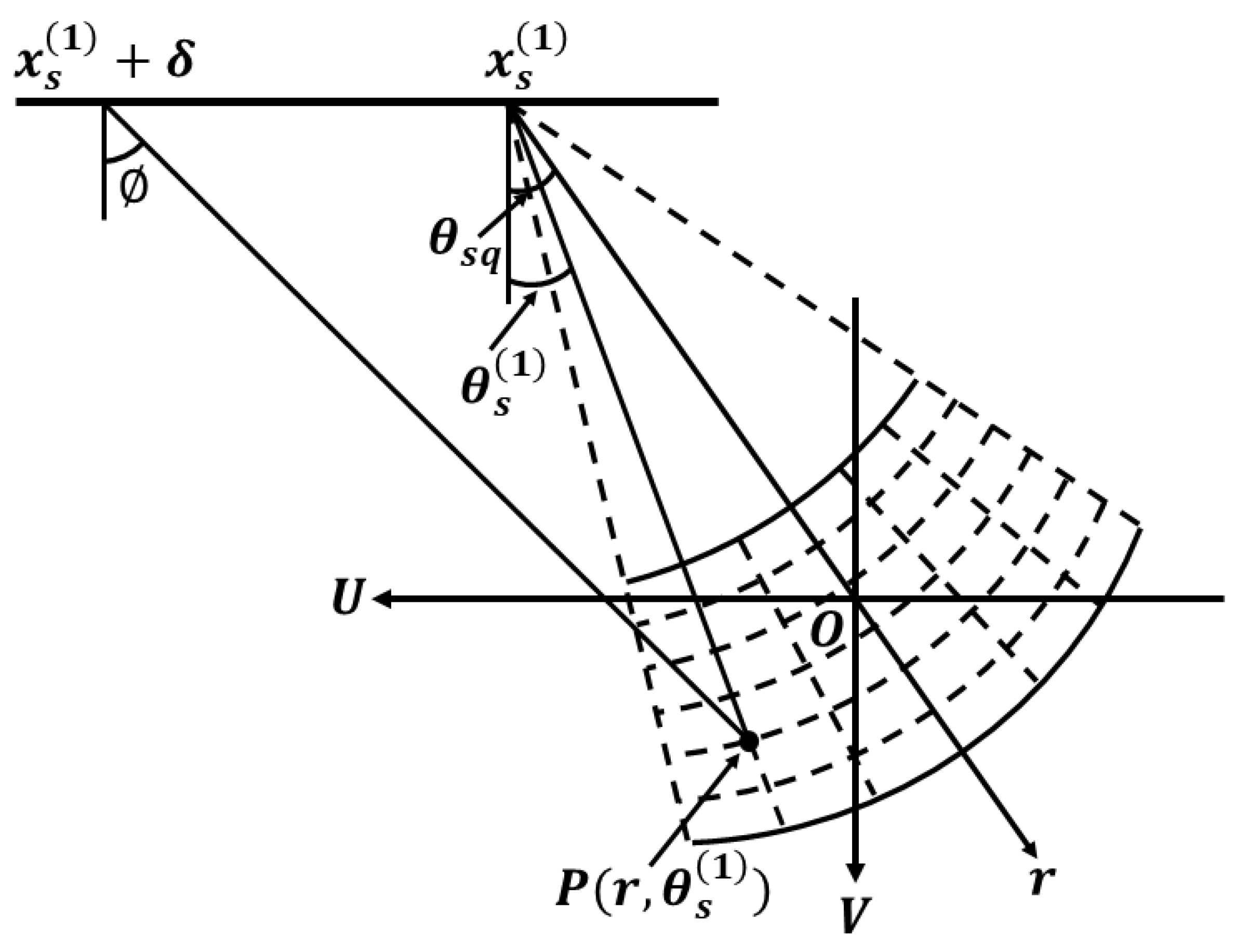
In the initial stage, shorter sub-apertures result in a lower angular domain sampling rate for the polar coordinate grid. This allows obtaining low-resolution sub-images in the angular domain with fewer sampling points, eliminating the need to back-project data corresponding to each aperture position to every pixel in the imaging grid. Consequently, this enhances the computational efficiency of the algorithm. As illustrated in Figure 1, for the s-th sub-aperture, a local polar coordinate system is established with as the origin. The sub-image can then be expressed as
where represents the instantaneous slant range from the aperture position to the pixel .
Subsequently, the current stage’s sub-images are obtained by coherent summation of the sub-images from the previous stage, that is
where the symbol “” denotes coherent accumulation. Coherent accumulation uses the phase relationship between the received pulses to add the phases of multiple coherent signal bands (complex data addition) and, finally, the signal amplitude accumulation and noise power accumulation, thereby improving the signal-to-noise ratio. Coherent accumulation allows the energy of all radar echoes to be added directly.
The differences between local polar coordinate systems result in , , and being situated in different local polar coordinate systems. Image recursive fusion requires establishing the mapping from the original coordinate systems and to the new coordinate system based on the geometric relationship between local polar coordinate systems. The specific implementation is a two-dimensional process dependent on distance and angular domain interpolation. As the length of sub-apertures increases, the number of sub-apertures decreases, and the angular domain spacing of sub-aperture images is continuously refined. After completing the processing of the K-th stage, where the length of sub-apertures equals the size of the entire aperture, the local polar coordinate systems are equivalent to the global polar coordinate system.
Finally, the polar coordinate system image is transformed back to the Cartesian coordinate system, yielding a full-space resolution image .
The aperture decomposition establishes an algorithmic structure similar to a butterfly operation, providing the foundation for the fast implementation of the FFBP algorithm. Beamforming is achieved at the signal processing level through the coherent accumulation of signals between sub-images, while recursive fusion, at the image fusion level, accomplishes the formation of angular domain resolution from low to high. Next, the FFBP algorithm will be applied to stripmap SAR processing.
2.2. Integral Aperture Determination
In spotlight SAR, the imaging scene is continuously covered by the beam throughout the entire synthetic aperture time. All the pixels to be reconstructed correspond to the same integration aperture (i.e., the entire aperture), and each aperture position contributes to the formation of pixels. In stripmap SAR, targets in the imaging scene are not continuously illuminated by the antenna beam during the synthetic aperture time. During the back-projection integration, different pixels correspond to different integration apertures. If range-compressed data are directly back-projected onto the entire imaging grid for integration, it not only causes incorrect accumulation of energy for pixels beyond the beam width, affecting imaging quality, but also increases computational complexity.
For the FFBP algorithm, the quality of sub-aperture images in the aperture segmentation stage directly determines the accuracy of subsequent stages in image recursive fusion. Therefore, it is crucial to introduce integral aperture determination during the sub-aperture back-projection integration process in the aperture segmentation stage.
Assuming the polar coordinates of a point P in the imaging scene are , and the azimuth coordinate from the radar’s initial position is . When the radar moves to , the direction from the antenna to point P is denoted as . The antenna beam can illuminate the point when the absolute value of the angle between and the line of sight direction is within the range of , i.e.,
Defining that satisfies Equation (4) as the integral aperture for point P, it can be denoted as . Once the integral apertures for each pixel on the imaging grid are known, the s-th sub-aperture image can be represented as
where is the instantaneous slant range from aperture position to pixel point .
After introducing integral aperture determination, the influence of the antenna pattern can be neglected. Through a similar sub-aperture back-projection integration method as in spotlight SAR, the integral apertures for all pixel points can be accurately determined. This enables the extension of the FFBP algorithm from spotlight SAR to stripmap SAR.
2.3. The Processing of Full-Aperture Data Blocks
Assuming the number of samples in the range direction of the imaging scene is M, and in the azimuth direction is N, and a single synthetic aperture contains L samples. The length of a single aperture is , and the maximum observable range in the azimuth direction is , as illustrated in Figure 2. It follows that the full resolution in the azimuth direction is . The total number of BP imaging operations within a complete aperture is given by
The FFBP process within a single full aperture involves K recursive operations, with a decomposition factor of 2 for each stage, so that L = 2K, assuming the range resolution of the image scene remains unchanged for each stage. In the first stage, the full aperture is divided into La/2 sub-apertures, each containing 2 azimuth samples, and using the echo data from each sub-aperture to form an image with coarse azimuth resolution. The number of BP operations in the first stage is given by
In the second stage, every two coarse images are merged together, resulting in a total of L/4 images with coarse azimuth resolution. The number of BP operations in the second stage is given by
After the second stage processing, the azimuthal sampling interval becomes half of the original, and the azimuthal resolution increases to twice the original.
Following this pattern, the number of BP operations in the K-th stage is given by
After K rounds of merging, the full-resolution image for a single full aperture can be obtained. The total number of BP operations for K stages is
Comparing Equation (6) with Equation (10), we have
Compared to direct BP, the computational speed of the FFBP algorithm is improved by a factor of L/(2log2L).
Next, the FFBP algorithm is applied to the continuous imaging of two full apertures. As shown in Figure 3, the two full apertures contain 2L samples with a length of 2La and a maximum observable distance in the azimuth direction of 3La.
For 2L = 2K+1, This process includes K + 1 stages, and the number of operations for each stage is as follows:
First stage
Second stage
Proceeding in this manner, the number of operations for the Kth stage is
At the Kth stage, the azimuth resolution of the image has already reached the optimum, and in the K + 1 stage, the resolution remains unchanged. Therefore, the number of BP operations for the (K + 1)th stage is
After K + 1 merging operations, the full-resolution images of the two full apertures can be obtained. The total number of FFBP operations is given by
The comparison between Equation (16) and Equation (10) reveals that
The aperture length has doubled, but the computational load has increased to three times that of processing a single aperture. The analysis reveals that the left full aperture has no effect on the rightmost imaging area, and similarly, the right full aperture has no effect on the leftmost imaging area. However, both have undergone integration operations, leading to redundancy.
Continue using the FFBP algorithm for continuous imaging of 3, 4, …, n full apertures. As shown in Figure 4, n full apertures contain nL samples with a length of nLa, and the maximum observable distance in the azimuthal direction becomes (n + 1)La.
Assuming nL = n2K ≤ 2K+x, such that the recursive iterations meet the imaging requirements, this process includes K + x stages, and the number of operations in each stage is as follows:
First stage
Second stage
Continuing in this manner, the number of computations in the Kth stage is
In the Kth stage, the azimuth resolution of the image has reached its optimum, and in the (K + 1)th, (K + 2)th, …, (K + x)th stage, the azimuth resolution will not increase further.
The number of BP operations in the (K + 1)th stage is
The number of BP operations in the (K + 2)th stage is
Continuing in this manner, the number of BP operations in the (K + x)th stage is
After K + x rounds of merging processing, n full-aperture full-resolution images can be obtained. The total number of FFBP operations is
Comparing Equation (24) with Equation (10), we can observe that
The aperture length has increased by a factor of n, but the computational workload has increased by a factor of more than n times compared to processing a single aperture. The increase in computational workload surpasses the increase in aperture length. With the increase in aperture length, the redundant calculations in the integration process become more significant, leading to a sharp increase in computational workload.
To address this issue, we can restrict the FFBP algorithm to process only one complete synthetic aperture at a time, i.e., the full-aperture data block. Subsequently, the results of processing all apertures are accumulated. Pixels in the currently synthetic aperture image with an integration aperture length smaller than the full aperture length can be compensated for by adjacent images. This ensures that the recovered integration aperture equals the true integration aperture, avoiding the underutilization of information. Processing the full-aperture data block also minimizes redundant calculations, improving computational efficiency and allowing for the efficient reconstruction of the image by fully utilizing all available information.
The total number of computations for processing the full-aperture data block is
Comparing Equation (26) with Equation (24), we can observe that
From Equation (27), it can be inferred that the processing efficiency for the full-aperture data block is approximately (n + 1)/2 times higher compared to directly using the FFBP algorithm for the continuous imaging of n full apertures.
2.4. Range Block Division
The digital spotlight algorithm can extract the SAR phase history data corresponding to the ROI (region of interest), and the extracted phase history data can be used for target recognition or other subsequent processing. Based on the Nyquist sampling theorem, the sampling rate of full-phase historical data is usually selected to sample the whole image without distortion. If the desired ROI is much smaller than the overall image size, then the Nyquist sampling requirement is greatly relaxed, i.e., the phase history of the ROI can be unambiguously sampled with much fewer samples than is required to generate the original SAR image, thus improving imaging efficiency.
A schematic diagram of the digital spotlight is shown in Figure 5. It is assumed that the existing phase history data can meet the needs of alias-free imaging in the green dotted circle area in Figure 5a. The center position of the scene is O, the position of the radar antenna is QC, and the historical frequency step and pulse repetition rate of the radar phase meet the alias-free imaging requirements in the area with a radius of R0. The goal of the digital spotlight algorithm is to reduce the size of the SAR phase historical data set, including the number of frequency samples and the number of pulses in azimuth, and to ensure alias-free imaging within the ROI around the new center C.
The first step of the digital spotlight algorithm requires determining the location and size of the ROI. The second step is to re-determine the phase history of the new center of the ROI, which is the SAR reference point of the new sub-image, and the third step is to “extract” the phase history data in the fast-time dimension. After the first three steps, a small distortion-free range can be obtained that is approximated by the red bold solid line contour area in Figure 5b, and the alias-free range distance is approximate to Wr, and the alias-free azimuth distance is Wx. The fourth step is to achieve uniform azimuth or angle by phase history interpolation. The final step is to “extract” the phase history data in the azimuth dimension, and eventually, the new phase history contains only the samples needed to generate an alias-free image of the ROI, as shown in the bold red solid outline area in Figure 5c.
Figure 6 provides a visualization of the phase history extraction in the fast- and slow-time dimensions. From Figure 6a, part of the phase history of frequencies and pulses occupies part of the annulus. Figure 6b shows that the extraction is performed with 2 as the extraction factor in the fast-time dimension. Figure 6c shows the extraction with 2 as the extraction factor in the slow-time dimension.
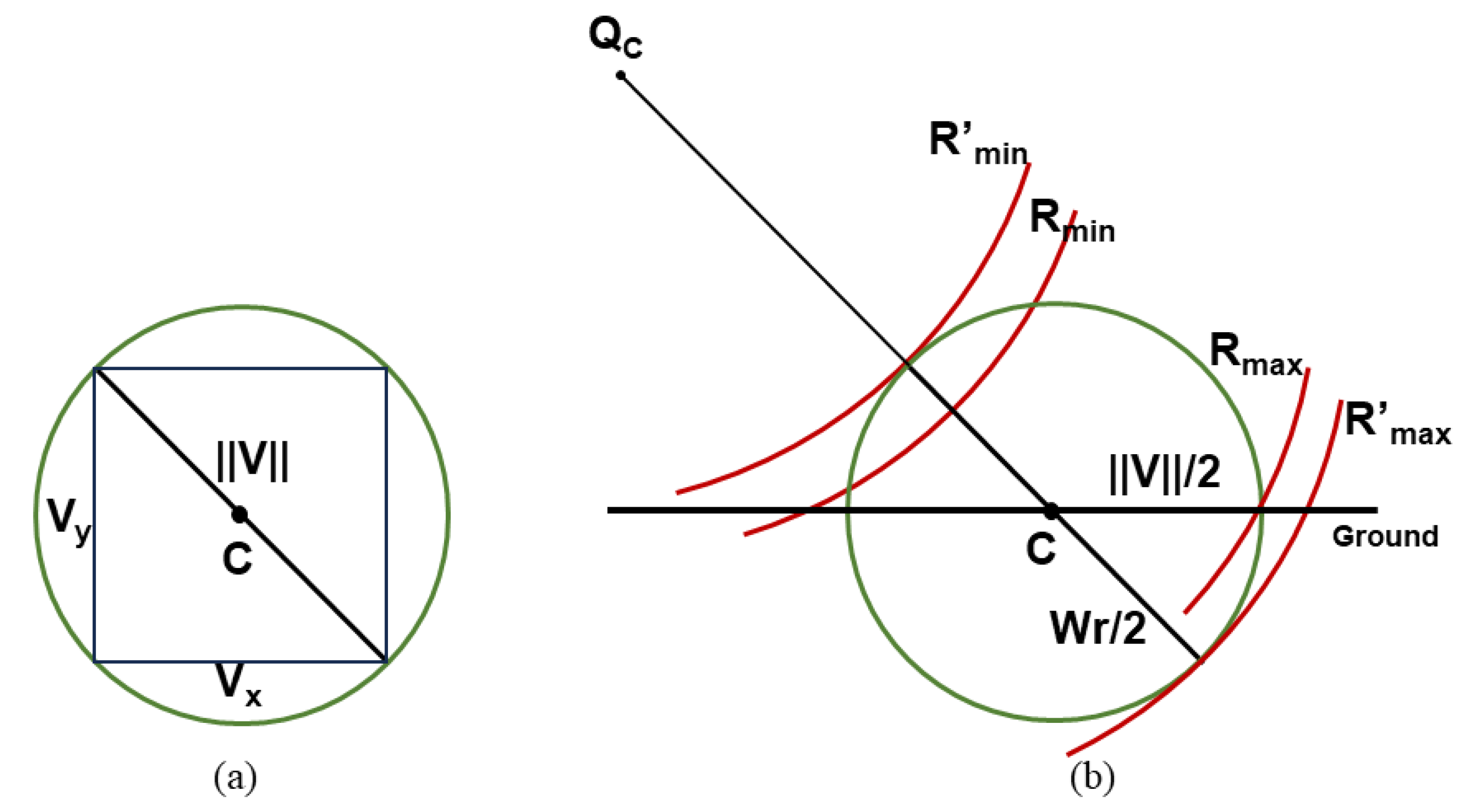
The digital spotlight range is specified using center offset C = [Cx,Cy,Cz] and a flat image area with a normal in the upper (z) direction and an edge length of V = [Vx,Vy]. Assuming that the center of the original image is [0,0,0], Figure 7a shows a flat image with an east–west side length of Vx and a north–south side length of Vy. A circle with diameter ||V|| on the ground (imaging plane) delineates the imaging area. As shown in Figure 7b, it is assumed that the alias-free distance Wr is equal to ||V||. The imaging area range is constrained by the maximum and minimum distance ranges Rmax and Rmin, which are located within the alias-free distance ranges R’max and R’min.
The frequency sampling vector {fk} has a minimum value of f1, a maximum value of fK, and a step size of Δf [23]. In the full phase history {Pk}, each complex phase history sample Pk is associated with fK, and Pk is the phase history sample within the range of the newly generated digital spotlight with a center of C. The difference in distance from the radar antenna to the origin and the radar antenna to the center of the digital spotlight is given by ΔR = R0 − Rc.
Equation (28) is used to correct K frequencies and Np pulses, and the result is a phase history that produces a C-centric ROI SAR image.
The ROI has a smaller alias-free range compared to the original whole scene, which can be met with a new frequency sampling interval Δf′ in Equation (29), and the alias-free range Wr is designed to be the same as the spotlight diameter ||V||.
Each pulse in the phase history can be decimated by an NDS factor to reduce the number of fast-time or frequency samples. Each pulse is decimated independently, making the decimation operation suitable for parallel processing.
The phase history data obtained after the above processing contain only the samples required to image the new scene in the range dimension, and the samples required to image other range dimensions have been deleted. All original samples remain unchanged in azimuth.
The radar pulse rate in SAR is usually specified by the pulse repetition rate (PRF). PRF, radar speed, and path produce a pulse-per-radian (PPR) pulse rate relative to the azimuth of the center of the spot. The PPR is related to the maximum alias-free span trajectory distance with azimuth spacing requirements
where kmax = ωmax/c = 2πfmax/c is the maximum wavenumber, Ø is the elevation angle (radian) from the center of the light to the radar antenna, and R0 is the radius of the spot area.
For a digital spotlight with radius R0, the desired alias-free distance length across the trajectory is Wx = 2R0, then the PPR requirement is
where Ø depends on the variable elevation angle between the center of the digital spotlight and the QC of the radar antenna on the radar path. To simplify, the PPR of a digital spotlight can be designed to be a constant related to the minimum elevation angle Ømin in the data block.
The radar antenna position of each pulse in the dataset is stored in meters on (east, north, up) or (x,y,z) Cartesian coordinate space. After converting these coordinates to spherical coordinates (azimuth, elevation, distance) relative to the center of focus, the azimuth information may have variable PPR with changes in relative motion path and velocity, so azimuth spacing Δθ is not constant. While the azimuth spacing can meet the requirements of Equation (31), the filtering algorithm requires a constant sample spacing that can interpolate the phase history to a uniform sample interval based on the smallest Δθ of the data blocks being processed. The purpose of “extracting” phase historical data in the slow-time dimension is to reduce the size of the dataset to match the smaller azimuth range of Wx < 2R0, so that Δθ′ is greater than Δθ, the required decimation factor is
After the extraction factor is selected, the phase history data block is extracted in the slow-time dimension. Finally, the SAR phase history data corresponding to the ROI is extracted, and the extracted phase history will be used for target identification or other subsequent processing.
The initial full-aperture phase historical data can be used to reconstruct alias-free SAR images in the area around the origin, and the proposed fast decomposition backward projection algorithm for strip SAR imaging based on range tiles takes the first three steps of the digital spotlight algorithm as the first stage of the “two-stage backward projection” image reconstruction process. Start by determining the location and size of the ROI. The phase history of the ROI center is then determined, which serves as the SAR reference point for the new image, and the third step is to “extract” the phase history data in the fast-time dimension. The main goal of DS technology is to decompose the phase history data into multiple parts in the distance upward, forming a smaller area of aliasing-free images around the new center. After a three-step process, the phase history data are decomposed into multiple parts in the distance upwards to form a smaller alias-free imaging area. Finally, the original full-aperture phase history data is filtered into multiple “pseudo” phase histories [24], and the imaging scene is segmented into multiple full-aperture sub-blocks along the distance, and the number of samples contained in each sub-block is greatly reduced, and the imaging efficiency is improved through parallel operation.
The aperture and image schematic are shown in Figure 2. Assuming the imaging scene size is MYG × NYG, where M and N are the number of samples in the range and azimuth directions, and M = N. YG represents the actual sampling interval.
Here, B is the bandwidth of the transmitted signal, f∆ is the frequency step size, and c is the speed of light.
Figure 8 gives a schematic diagram of range block division imaging. There are N × N pixels in the original imaging area, and the center of the whole large scene is denoted as O(X0,Y0,Z0), wherein X0 is in the range dimension, Y0 is in the azimuth dimension, and Z0 is the height. The entire imaging area is divided into D subregions in the distance direction by the digital spotlight method, and each subregion contains N × (N/D) pixels. The center O of the original large scene is taken as the reference point, and the center point of the sub-scene (i,j) is , is in the range dimension, and is in the azimuth dimension
where i, j are the indexes of the matrix columns and rows, respectively, and i = 1, j∊[1, D] indicates that the azimuth dimension is not divided, and the range dimension is divided into D subblocks. In Figure 8, D = 4, the whole imaging scene is divided into four sub-scenes in the distance direction, which are denoted as Sub-sence1, Sub-sence2, Sub-sence3 and Sub-sence4, respectively, and the sub-scene center points corresponding to the four sub-scenes are C1, C2, C3 and C4, respectively. Assuming that the imaging scene is on the ground, Z0 = 0 and the center of the large scene is O (X0,Y0,0).
Calculate the distance of the center point of the above sub-scene (i,j) relative to the center O of the original large imaging scene
Taking the center O of the original large scene as the reference point, the position of the radar antenna (relative to the center O of the original large scene) at a certain time is denoted as QC (X,Y,Z), where X is in the range dimension, Y is in the azimuth dimension, and Z is the height. Assuming that the imaging scene is on the ground, so Z0 = 0, the radar antenna position is QC (X,Y,0). As the radar platform moves, the antenna position is constantly moving in the azimuth direction, marked as a continuously moving red dot in Figure 8. For each pulse return of the phase history, the position of the antenna must be updated to reflect the position of the new sub-scene center. The new antenna position (relative to the new scene center Cj) is
where
In order to place the digital spotlight scene at zero frequency, it is necessary to obtain the new center phase history through phase shifting. First, calculate the differential range from the digital spotlight center Cj to the scene center O.
The phase history for the new center is
where f[k] = fc − B/2 + f∆q, Xph[∙] is the original phase history data of the scene, and Xph[∙] is the phase history data after recentering at position C. Applying low-pass filtering to the recentered data yields
where Fπ/D{∙} is the low-pass filtering operation with a discrete cutoff frequency applied to ωc = π/D. The processed data can then be downsampled by a factor of D.
where Xrd,i,j[∙] is the phase history extracted in the range direction from the imaging area.
After the above operation, the phase history data of the entire original scene are “extracted” in the distance or fast-time dimension, and the result contains only the samples needed to image the new sub-scene. The gray area in Figure 8 represents the result of an “extraction”, all the original samples remain unchanged in the azimuth direction, and the distance to the sample is “extracted” to 1/4 of the original sample, and only the sample points required for imaging in sub-scene 1 are retained, and the samples required for imaging other distance positions (sub-scene 2, sub-scene 3 and sub-scene 4) in the original scene are deleted. The remaining 3 sub-scenes are treated similarly. After 4 times of “extraction”, the “extraction” result traverses all samples in the original imaging scene, ensuring that the original scene can be imaged without distortion, and the imaging efficiency can be improved through parallel computing.
In summary, the fast factorized back-projection algorithm based on range block division for stripmap SAR imaging consists of the following steps:
- (1)
- The received signal data is divided into multiple sub-blocks along the range direction by using the range block technology;
- (2)
- The obtained sub-block data is further decomposed into multiple full-aperture sub-block data in the azimuth direction according to the sub-aperture judgment and full-aperture data block processing principles mentioned in Section 2.2 and Section 2.3;
- (3)
- The FFBP algorithm is used to image the data of each full-aperture sub-block;
- (4)
- All full-aperture sub-block images are superimposed to obtain alias-free SAR images in the whole large scene.
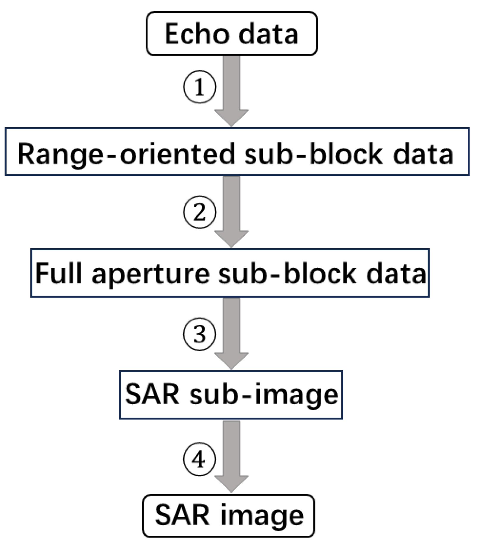
The flow chart of the fast factorized back-projection algorithm based on range block division for stripmap SAR imaging is shown in Figure 9.
Among them, ① represents range block technology, ② represents sub-aperture judgment and full-aperture data block processing, ③ represents FFBP algorithm imaging, and ④ represents sub-image overlay.
After the above steps, the integrated aperture judgment expands the FFBP algorithm from beam gathering to strips, the full-aperture data block processing can reduce redundant calculations, the distance block decomposition can further reduce the number of backward projection operations in each sub-scene, and finally, each sub-scene is imaged through parallel operation, so as to improve the computing efficiency of the whole imaging process.
3. Results
In this section, the results of the point target simulation and the experimental results of the raw data are given and analyzed to evaluate the performance of the proposed algorithm. The algorithms for both simulation and raw data experiments are programmed on a MATLAB platform and Windows 10 system.
3.1. Simulation Experiments
A set of vehicle-mounted strip SAR simulation parameters were designed for point target performance analysis, with specific parameters as shown in Table 1.
Set five target points, as shown in Figure 10; the coordinates of the target points from left to right (azimuth, range) are (,), (,), (0,), (,), (,), = 2000 m is the horizontal distance between the imaging center and the radar. = 50 m, = 100 m. The point target imaging results are shown in Figure 11.
To analyze the imaging in more detail, the direct BP, FBP, FFBP, and the fast factorized back-projection algorithm based on range block division are used to simulate the nadir target in Figure 10. The coordinates of this point are (0,). The results are shown in Figure 12. The parameters measured by the results of each algorithm are shown in Table 2.
The calculation of azimuth resolution is expressed as
where λ = c/fc is the radar wavelength, fc is the radio frequency carrier frequency, and L is the aperture length (synthetic aperture). Assume that the bedrock interface depth inside the glacier is d = 2000 m and the synthetic aperture length is 200 m. According to the parameters in Table 1 and Equation (45), the theoretical azimuth resolution ρA = 5.27 m can be calculated. According to Figure 12b, the azimuth resolution obtained by measuring the 3 dB width is 5.95 m, and the peak side lobe ratio in the azimuth direction is –13.8482 dB; according to Figure 12d, the azimuth resolution obtained by measuring the 3dB width is 6.03 m, the peak side/lobe ratio in the azimuth direction is −14.0577 dB; according to Figure 12f, the azimuth resolution obtained by measuring the 3 dB width is 5.99 m, and the peak side/lobe ratio in the azimuth direction is −13.9722 dB; according to Figure 12h, the azimuth resolution obtained by measuring the 3 dB width is 6.54 m, and the peak side/lobe ratio in the azimuth direction is −13.9359 dB. It can be seen that the algorithm proposed in this article has essentially the same azimuthal resolution with direct back-projection.
Next, the imaging time of point targets based on BP, FBP, FFBP, and the fast factorized back-projection algorithm based on range block division is compared and analyzed. The simulation point is still the nadir target in Figure 6, and the coordinates of this point are (0,−rc). The imaging time of the BP algorithm is 2999.808 s, that of the FBP algorithm is 451.098 s, that of the FFBP algorithm is 326.198 s, and that of the fast factorized back-projection algorithm based on range block division is 160.440 s. Based on the imaging time of the BP algorithm (the acceleration ratio is 1), the acceleration ratio of the FBP algorithm is 6.65, the acceleration ratio of the FFBP algorithm is 9.19, and the acceleration ratio of the fast factorized back-projection algorithm based on range block division for stripmap SAR is 18.70. This is shown in Table 3.
Compared with direct BP imaging, the imaging efficiency of FBP, FFBP, and the fast factorized back-projection algorithm based on range block division for stripmap SAR is greatly improved compared with direct BP imaging. Compared with the FFBP algorithm, the imaging efficiency of the fast factorized back-projection algorithm based on range block division for stripmap SAR proposed in this paper has been further improved. Through the comparative analysis of the performance and imaging time of the point target, the reliability and efficiency of the fast factorized back-projection algorithm based on range block division for stripmap SAR are verified.
3.2. Raw Data Experiments
This section demonstrates the effectiveness of the proposed ultra-wideband ice radar imaging algorithm based on fast factorized back-projection using real measurement data from a multi-channel ice radar provided by the Ice Radar Center at the University of Kansas. Key parameters are provided in Table 1. The data shown in Figure 13 represent ultra-wideband ice radar data obtained from the Greenland Ice Sheet, from T1 (72°36′35″ N, 37°38′3″ W) to T1′ (72°36′29″ N, 38°19′19″ W) and T2 (72.5806° N, 38.4133° W) to T2′ (72.5832° N, 37.4453° W).
Figure 14 and Figure 15 show SAR imaging results from two different lines. Both lines extend in an east–west direction, with line T1T1′ running from east to west and line T2T2′ running from west to east, with a distance of 500 m in the north–south direction. Figure 14a and Figure 15a are processing results of the FFBP algorithm. Figure 14b and Figure 15b are processing results of the fast factorized back-projection algorithm based on range block division. A comparison was made between the proposed algorithm and the FFBP algorithm, demonstrating the computational advantages of this algorithm. The computation times for Figure 14a,b are 5742 s and 3588 s, respectively, while the computation times for Figure 15a,b are 7509 s and 4446 s, respectively. The algorithm proposed in this paper is superior to the FFBP algorithm. Through the comparison of computation time, it can be concluded that the proposed algorithm can significantly reduce the amount of computation required for imaging ice radar data and achieves nearly the same imaging effects and azimuth resolution as the FFBP algorithm.
4. Conclusions
In this paper, we propose a fast factorized back-projection algorithm based on range block division for stripmap SAR imaging, combined with digital spotlight technology, to divide the full-aperture echo data into several sub-blocks in the range direction. Each sub-block contains a smaller number of samples than the original data, and then FFBP processing is carried out on the full-aperture sub-blocks, respectively, which significantly reduces the number of back-projection operations and improves the computational efficiency through parallel operation.
This paper reviews the basic principles of the FFBP algorithm, describes the problems of unclear integrated aperture and computational redundancy encountered in the direct application of the FFBP algorithm to strip SAR processing, and proposes corresponding solutions to these problems (i.e., integrated aperture judgment and full-aperture data block processing), and then analyzes the principles of integrated aperture judgment and full-aperture data block processing. The amount of computation is calculated, and the introduction of integrated aperture judgment can ensure that the imaging quality is not affected and the computational cost can be minimized for a single complete aperture processing. The digital spotlight technology is then used to further improve the imaging efficiency through range block operation. Through the point target simulation experiment, the point target imaging performance and imaging time of four different algorithms are compared, and the efficiency of the algorithm in the strip SAR point target simulation imaging is verified. The measured data of vehicle-mounted multi-channel ice radar provided by the University of Kansas Ice Sheet Remote Sensing Center are processed, and the feasibility and efficiency of the proposed fast factorized back-projection algorithm based on range block division for stripmap SAR imaging are further verified by comparing the imaging time of different algorithms. This algorithm has a certain degree of flexibility in practical application, can be applied to the data collected by vehicle-mounted ultra-wideband ice radar, and can be used for imaging operations more efficiently through further reasonable division of range.
Author Contributions
Conceptualization, Y.W.; methodology, Y.W.; software, Y.W.; validation, Y.W.; formal analysis, Y.W.; investigation, Y.W. and B.L.; resources, B.Z.; data curation, Y.W. and B.L.; writing—original draft preparation, Y.W.; writing—review and editing, Y.W. and B.L.; visualization, Y.W.; supervision, B.Z.; project administration, B.Z. and X.L.; funding acquisition, B.Z. and X.L. All authors have read and agreed to the published version of the manuscript.
Funding
This research was funded by the National Key Research and Development Program of China, grant number 2023YFF1303500.
Data Availability Statement
Data available on request due to restrictions.
Acknowledgments
The authors would like to thank the editors and reviewers for their efforts in helping with the publication of this work.
Conflicts of Interest
The authors declare no conflicts of interest.
References
- Cumming, I.G.; Wong, F.H. Digital processing of synthetic aperture radar data. Artech House 2005, 1, 108–110. [Google Scholar]
- Wu, C. A digital system to produce imagery from SAR data. In Systems Design Driven by Sensors; AIAA: Pasadena, CA, USA, 1976; p. 968. [Google Scholar]
- Cafforio, C.; Prati, C.; Rocca, F. SAR data focusing using seismic migration techniques. IEEE Trans. Aerosp. Electron. Syst. 1991, 27, 194–207. [Google Scholar] [CrossRef]
- Raney, R.K.; Runge, H.; Bamler, R.; Cumming, I.G.; Wong, F.H. Precision SAR processing using chirp scaling. IEEE Trans. Geosci. Remote Sens. 1994, 32, 786–799. [Google Scholar] [CrossRef]
- Soumekh, M. Synthetic Aperture Radar Signal Processing; Wiley: New York, NY, USA, 1999; Volume 7. [Google Scholar]
- Meng, D.; Hu, D.; Ding, C. Precise focusing of airborne SAR data with wide apertures large trajectory deviations: A chirp modulated back-projection approach. IEEE Trans. Geosci. Remote Sens. 2014, 53, 2510–2519. [Google Scholar] [CrossRef]
- Desai, M.D.; Jenkins, W.K. Convolution back-projection image reconstruction for spotlight mode synthetic aperture radar. IEEE Trans. Image Process. 1992, 1, 505–517. [Google Scholar] [CrossRef]
- Yegulalp, A.F. Fast back-projection algorithm for synthetic aperture radar. In Proceedings of the 1999 IEEE Radar Conference. Radar into the Next Millennium (Cat. No. 99CH36249), Waltham, MA, USA, 22 April 1999; pp. 60–65. [Google Scholar]
- Ulander, L.M.; Hellsten, H.; Stenstrom, G. Synthetic-aperture radar processing using fast factorized back-projection. IEEE Trans. Aerosp. Electron. Syst. 2003, 39, 760–776. [Google Scholar] [CrossRef]
- Li, Y.; Xu, G.; Zhou, S.; Xing, M.; Song, X. A novel CFFBP algorithm with non-interpolation image merging for bistatic forward-looking SAR focusing. IEEE Trans. Geosci. Remote Sens. 2022, 60, 5225916. [Google Scholar]
- Zhang, L.; Li, H.-l.; Qiao, Z.-j.; Xu, Z.-w. A fast BP algorithm with wavenumber spectrum fusion for high-resolution spotlight SAR imaging. IEEE Geosci. Remote Sens. Lett. 2014, 11, 1460–1464. [Google Scholar] [CrossRef]
- Xie, H.; Shi, S.; An, D.; Wang, G.; Wang, G.; Xiao, H.; Huang, X.; Zhou, Z.; Xie, C.; Wang, F. Fast factorized back-projection algorithm for one-stationary bistatic spotlight circular SAR image formation. IEEE J. Sel. Top. Appl. Earth Obs. Remote Sens. 2017, 10, 1494–1510. [Google Scholar] [CrossRef]
- Ran, L.; Liu, Z.; Li, T.; Xie, R.; Zhang, L. An adaptive fast factorized back-projection algorithm with integrated target detection technique for high-resolution and high-squint spotlight SAR imagery. IEEE J. Sel. Top. Appl. Earth Obs. Remote Sens. 2017, 11, 171–183. [Google Scholar] [CrossRef]
- Dong, Q.; Sun, G.-C.; Yang, Z.; Guo, L.; Xing, M. Cartesian factorized back-projection algorithm for high-resolution spotlight SAR imaging. IEEE Sens. J. 2017, 18, 1160–1168. [Google Scholar] [CrossRef]
- Ulander, L.; Frölind, P.-O.; Murdin, D. Fast factorised back-projection algorithm for processing of microwave SAR data. In Proceedings of the EUSAR, Dresden, Germany, 16–18 May 2006; pp. 577–580. [Google Scholar]
- Moon, K.; Long, D.G. A new factorized back-projection algorithm for stripmap synthetic aperture radar. Positioning 2013, 4, 28383. [Google Scholar] [CrossRef]
- Hao-lin, L.; Lei, Z.; Meng-dao, X.; Zheng, B. Innovative strategy for stripmap SAR imaging using fast factorized back-projection. J. Electron. Inf. Technol. 2015, 37, 1808–1813. [Google Scholar]
- Xu, G.; Zhou, S.; Yang, L.; Deng, S.; Wang, Y.; Xing, M. Efficient fast time-domain processing framework for airborne bistatic SAR continuous imaging integrated with data-driven motion compensation. IEEE Trans. Geosci. Remote Sens. 2021, 60, 5208915. [Google Scholar] [CrossRef]
- Dungan, K.E.; Gorham, L.A.; Moore, L.J. SAR digital spotlight implementation in MATLAB. In Algorithms for Synthetic Aperture Radar Imagery XX; SPIE: Bellingham, WA, USA, 2013; pp. 80–90. [Google Scholar]
- Nguyen, L.; Ressler, M.; Wong, D.; Soumekh, M. Enhancement of back-projection SAR imagery using digital spotlighting preprocessing. In Proceedings of the 2004 IEEE Radar Conference (IEEE Cat. No. 04CH37509), Philadelphia, PA, USA, 29 April 2004; pp. 53–58. [Google Scholar]
- Balster, E.J.; Mundy, D.B.; Kordik, A.M.; Hill, K.L. Digital spotlighting parameter evaluation for SAR imaging. In Proceedings of the 2017 Seventh International Conference on Image Processing Theory, Tools and Applications (IPTA), Montreal, QC, Canada, 28 November–1 December 2017; pp. 1–6. [Google Scholar]
- Nie, X.; Lei, W.; Zhuang, L. A two-step wide-scene polar format algorithm for high-resolution highly-squinted SAR. IEEE Geosci. Remote Sens. Lett. 2022, 19, 4503405. [Google Scholar] [CrossRef]
- Gorham, L.A.; Moore, L.J. SAR image formation toolbox for MATLAB. In Proceedings of the Algorithms for Synthetic Aperture Radar Imagery XVII; SPIE: Bellingham, WA, USA, 2010; pp. 46–58. [Google Scholar]
- Farhadi, M.; Feger, R.; Fink, J.; Gonser, M.; Hasch, J.; Stelzer, A. Adaption of fast factorized back-projection to automotive SAR applications. In Proceedings of the 2019 16th European Radar Conference (EuRAD), Paris, France, 2–4 October 2019; pp. 261–264. [Google Scholar]
Figure 1.
The local polar coordinate grid of the k-th sub-aperture in the first stage.

Figure 2.
Concept of full aperture.

Figure 3.
Concept of two full apertures.

Figure 4.
Concept of n full apertures.

Figure 5.
Schematic diagram of a digital spotlight: (a) Upon recentering and fast time, or frequency, decimation; (b) The alias-free range is reduced to the desired digital spotlight. Slow time, or pulse rate, decimation; (c) reduces the alias-free cross-range as well.
Figure 5.
Schematic diagram of a digital spotlight: (a) Upon recentering and fast time, or frequency, decimation; (b) The alias-free range is reduced to the desired digital spotlight. Slow time, or pulse rate, decimation; (c) reduces the alias-free cross-range as well.

Figure 6.
Visualization of phase history extraction in the fast- and slow-time dimensions: (a) Frequency decimation; (b) Reduces the alias-free range and slow time decimation; (c) across frequency bins reduces the alias-free cross-range.
Figure 6.
Visualization of phase history extraction in the fast- and slow-time dimensions: (a) Frequency decimation; (b) Reduces the alias-free range and slow time decimation; (c) across frequency bins reduces the alias-free cross-range.

Figure 7.
Flat and side views of the digital spotlight processing area: (a) From the side view; (b) The alias-free range Wr is designed to exceed the image plane diameter ||V||.
Figure 7.
Flat and side views of the digital spotlight processing area: (a) From the side view; (b) The alias-free range Wr is designed to exceed the image plane diameter ||V||.

Figure 8.
Schematic diagram of range block division.

Figure 9.
The flow chart of the fast factorized back-projection algorithm based on range block division for stripmap SAR imaging.
Figure 9.
The flow chart of the fast factorized back-projection algorithm based on range block division for stripmap SAR imaging.

Figure 10.
Position of targets used in the simulation.

Figure 11.
The point target imaging results using the fast factorized back-projection algorithm based on range block division.
Figure 11.
The point target imaging results using the fast factorized back-projection algorithm based on range block division.

Figure 12.
Point target range and azimuth profiles: (a,b) are the range and azimuth profiles processed by the direct backward projection algorithm; (c,d) are the range and azimuth profiles processed by the FBP algorithm; (e,f) are the range and azimuth profiles processed by the FFBP algorithm; (g,h) are the range and azimuth profiles processed by the fast factorized back-projection algorithm based on range block division.


Figure 13.
Location of tracks processed in this article.

Figure 14.
Experimental results of two algorithms for survey line T1T1′: (a) FFBP; (b) the fast factorized back-projection algorithm based on range block division.
Figure 14.
Experimental results of two algorithms for survey line T1T1′: (a) FFBP; (b) the fast factorized back-projection algorithm based on range block division.

Figure 15.
Experimental results of two algorithms for survey line T2T2′: (a) FFBP; (b) the fast factorized back-projection algorithm based on range block division.
Figure 15.
Experimental results of two algorithms for survey line T2T2′: (a) FFBP; (b) the fast factorized back-projection algorithm based on range block division.


Table 1.
SAR parameters in simulation.
| Parameter Name | Value | Units |
|---|---|---|
| Mode | Stripmap | |
| Carrier frequency | 160 | MHz |
| Transmitted pulse period | 10 | μs |
| Signal bandwidth | 80 | MHZ |
| Range sampling rate | 720 | MHZ |
| PRF | 6910 | Hz |
| Radar platform average velocity | 3 | m/s |
Table 2.
Point target performance analysis.
| Range | Azimuth | |||
|---|---|---|---|---|
| PSLR (dB) | ISLR (dB) | PSLR (dB) | ISLR (dB) | |
| BP | −13.8732 | −11.1236 | −13.8482 | −10.7905 |
| FBP | −13.8633 | −11.2107 | −14.0577 | −10.8815 |
| FFBP | −13.7951 | −11.2417 | −13.9722 | −10.9766 |
| The proposed algorithm | −13.785 | −11.1250 | −13.9359 | −10.9368 |
Table 3.
Imaging time and acceleration ratio of different algorithms.
| The Name of the Algorithm | Imaging Time (s) and Acceleration Ratio (Times) | |
|---|---|---|
| BP | 2999.808 | 1 |
| FBP | 451.098 | 6.65 |
| FFBP | 326.198 | 9.19 |
| The proposed algorithm | 160.44 | 18.70 |
Disclaimer/Publisher’s Note: The statements, opinions and data contained in all publications are solely those of the individual author(s) and contributor(s) and not of MDPI and/or the editor(s). MDPI and/or the editor(s) disclaim responsibility for any injury to people or property resulting from any ideas, methods, instructions or products referred to in the content. |
© 2024 by the authors. Licensee MDPI, Basel, Switzerland. This article is an open access article distributed under the terms and conditions of the Creative Commons Attribution (CC BY) license (https://creativecommons.org/licenses/by/4.0/).
Share and Cite
MDPI and ACS Style
Wu, Y.; Li, B.; Zhao, B.; Liu, X. A Fast Factorized Back-Projection Algorithm Based on Range Block Division for Stripmap SAR. Electronics 2024, 13, 1584. https://doi.org/10.3390/electronics13081584
AMA Style
Wu Y, Li B, Zhao B, Liu X. A Fast Factorized Back-Projection Algorithm Based on Range Block Division for Stripmap SAR. Electronics. 2024; 13(8):1584. https://doi.org/10.3390/electronics13081584
Chicago/Turabian StyleWu, Yawei, Binbin Li, Bo Zhao, and Xiaojun Liu. 2024. "A Fast Factorized Back-Projection Algorithm Based on Range Block Division for Stripmap SAR" Electronics 13, no. 8: 1584. https://doi.org/10.3390/electronics13081584
Note that from the first issue of 2016, this journal uses article numbers instead of page numbers. See further details here.