LaANIL: ANIL with Look-Ahead Meta-Optimization and Data Parallelism

Abstract

Meta-few-shot learning algorithms, such as Model-Agnostic Meta-Learning (MAML) and Almost No Inner Loop (ANIL), enable machines to learn complex tasks quickly with limited data and based on previous experience. By maintaining the inner loop head of the neural network, ANIL leads to simpler computations and reduces the complexity of MAML. Despite its benefits, ANIL suffers from issues like accuracy variance, slow initial learning, and overfitting, hardening its adaptation and generalization. This work proposes “Look-Ahead ANIL” (LaANIL), an enhancement to ANIL for better learning. LaANIL reorganizes ANIL’s internal architecture, integrating parallel computing techniques (to process multiple training examples simultaneously across computing units) and incorporating Nesterov momentum (which accelerates convergence by adjusting the learning rate based on past gradient information and extracting informative features for look-ahead gradient computation). These additional features make our model more state-of-the-art capable and better edge-compatible and thus improve few-short learning by enabling models to quickly adapt to new information and tasks. LaANIL’s effectiveness is validated on established meta-few-shot learning datasets, including FC100, CIFAR-FS, Mini-ImageNet, CUBirds-200-2011, and Tiered-ImageNet. The proposed model achieved an increased validation accuracy by 7 ± 0.7% and a variance reduction by 44 ± 4% in two-way two-shot classification as well as increased validation by 5 ± 0.4% and a variance reduction by 18 ± 2% in five-way five-shot classification on the FC100 dataset and similarly performed well on other datasets.

1. Introduction

Meta-learning, or the process of learning how to learn, involves systematically observing the performance of various machine learning approaches across a range of learning tasks and subsequently using this experience or “meta-data” to rapidly learn new tasks [1]. When acquiring new competencies, it is unusual to begin from scratch; instead, we build upon our existing knowledge, drawing from previously acquired skills, reusing successful strategies, and prioritizing potentially valuable techniques based on experience. Thus, acquiring a new skill becomes simpler, requiring fewer examples and less trial and error. Essentially, we learn how to learn across a range of tasks [1].

Meta-few-shot image classification is a specific technique in the field of machine learning that combines the principles of few-shot learning and meta-learning. Few-shot learning focuses on training models to identify new objects with a limited number of examples, while meta-learning involves teaching models to quickly learn new skills or knowledge. Meta-few-shot image classification combines these two techniques, allowing models to quickly adapt to new objects with minimal data [2]. Moreover, this approach enables machines to rapidly comprehend complex concepts, which is facilitated by modern meta-learning algorithms such as Model-Agnostic Meta-learning (MAML) [3] and its derivative, Almost No Inner Loop (ANIL) [4]. The main innovation of ANIL is its simplified method that only retains the classification head of the inner loop while keeping frozen the other layers of the inner loop from the MAML design. While ANIL offers a streamlined architecture and inherent computational advantages, it faces significant challenges that hinder its flexibility and generalizability in the context of meta-learning. These obstacles may include limitations in handling diverse and complex data types, difficulties in adapting to new and unseen scenarios with fewer data, and challenges in effectively transferring knowledge across different domains [5].

This work proposes an updated algorithmic approach aimed at overcoming deficiencies and increasing the effectiveness of ANIL in real-world scenarios. By reorganizing ANIL’s internal architecture, integrating parallel computing techniques [6], and incorporating Nesterov momentum [7] for optimized look-ahead gradient calculations, this stabilization technique amplifies the model’s ability to adapt quickly in dynamic environments. In sum, these modifications aid in honing task-specific adaptation, resulting in faster responsiveness and more widespread generalization. Integrating data parallelism with Nesterov’s momentum can significantly improve the speed and accuracy of model convergence [8,9]. The former splits data across multiple processors and uses multiple model instances to efficiently estimate gradients [10]. Nesterov’s momentum, which predicts gradient direction for better update adjustments, benefits from this improved estimation. During the training and adaptation phases, they work together synergistically to enhance the model’s responsiveness and accelerate convergence [11]. Our proposed model was thoroughly validated on well-known public meta-few-shot learning datasets, including the benchmark datasets FC100 CIFAR-FS, Mini-ImageNet, CUBirds-200-2011, and Tiered-ImageNet, demonstrating notable results.

The choice of few-shot image classification as the evaluation benchmark is supported by the following reasons [12]:

• Real-world relevance: We chose few-shot image classification to demonstrate LaANIL’s ability to learn from a limited number of examples, which mimics real-world scenarios where acquiring extensive labeled data is often unfeasible.
• Generalization and adaptability: Few-shot image classification tasks require models to quickly adapt to new classes with only a small number of examples per class. This demonstrates the model’s ability to generalize from limited information, a crucial attribute for incremental learning algorithms like LaANIL, which are designed to assimilate and accommodate new knowledge iteratively.
• Robustness and flexibility: The use of few-shot image classification as the evaluation metric highlights the importance of models being able to learn from minimal data, which is in line with the fundamental goals of incremental learning frameworks.
• Benchmarking against state-of-the-art: Few-shot image classification tasks are used as a standardized benchmark to evaluate the performance of new algorithms. LaANIL was subjected to this benchmark to effectively compare its performance against state-of-the-art few-shot learning methods and assess its effectiveness in handling limited-data scenarios.
• Addressing model bias and overfitting: Few-shot image classification requires models to effectively combat overfitting and bias due to the limited training samples, which may lead to skewed representations.

The rest of the paper is organized as follows: Section 2 presents an introduction to meta-learning, MAML, and ANIL, along with their advantages and disadvantages. Section 3 describes our proposal. Section 4 presents the experiments we have performed and Section 5 discusses the results. The manuscript ends with some conclusions and further lines of research.

2. Background

2.1. Meta-Learning

Meta-learning [8] is a technique where a model learns how to learn, enabling it to adapt quickly to new tasks or datasets with minimal data [1]. The term meta-learning covers any type of learning based on prior experience with other tasks. The more similar those previous tasks are, the more types of meta-data we can leverage, and defining task similarity will be a key overarching challenge [13].

Meta-learning is, however, not a recent idea, and it has had many names in the past, such as meta-modeling, learning to learn, continuous learning, ensemble learning, and transfer learning. This large and growing body of work has demonstrated that meta-learning can drastically make machine learning more efficient, accessible, and trustworthy. Recent meta-learning techniques, such as meta-descent in optimization, meta-reinforcement learning in reinforcement learning, and meta-few-shot learning, have been developed when labeled data are scarce. Metric-based, model-based, and optimization-based meta-learning are the three major categories of meta-learning [14].

Meta-learning improves deep learning models by enabling them to learn from a variety of tasks, enhancing their ability to quickly adapt to new and unseen tasks with minimal additional data. In contrast, conventional deep learning has many limitations, including the inability to learn new tasks as quickly as humans do when drawing on prior experience, and many classifiers require massive amounts of training data [15]. Furthermore, deep learning algorithm performance depends heavily on labeled data with predefined attributes, which sometimes restricts generalization. Researchers have proposed remedies for this problem (e.g., transfer learning) through the use of trained models. However, inadequate pre-training data, test data that vary from the pre-training data, samples of particular classes that are too small, and other issues lead to poor model performance throughout the learning process, which is addressed by meta-learning [14].

Meta-few-shot image classification (a particularly challenging meta-learning problem that requires training an accurate deep learning model using only a few training examples [13]), a recent state-of-the-art meta-learning technique, employs the learn-to-learn approach for high adaptability to new tasks and reliability across different hardware configurations [4]. It has achieved exceptional performance in computer vision, robotics, and language processing due to its innate multitasking ability and rapid adaptability. This method, which involves training an accurate deep learning model with only a few training examples, is critical in diverse fields. These include computer vision applications for image classification, advanced driver assistant systems (ADAS) for object identification [16], agriculture for plant classification [17], as well as natural language processing and healthcare sectors.

2.2. Model-Agnostic Meta-Learning (MAML)

MAML [3] is a leading method in optimization-based meta-learning. It employs second-order computations (see Figure 1a) to learn across tasks taken from the same distribution. The system utilizes a blend of two nested cycles to optimize (i.e., bi-level optimization), and it aims to enhance overall proficiency [18].

$${\theta }^{*}=argmin\frac{1}{M}\sum _{i=1}^{M}L\left(in(\theta ,D_i^{tr})D_i^{test}\right)$$

(1)

The individual terms in Equation (1) are as follows: M denotes the number of tasks in the group and $D_i^{tr}$ and $D_i^{test}$ denote the $i^{th}$ task in the training and test sets, respectively. The function L denotes the task loss, and the function in $D_i^{tr}$ denotes the inner loop training data. The neural network is started with $\theta$ for each job in a batch. This value is optimized in the inner loop for one or a few gradient descent training steps on the training set $D_i^{tr}$ to acquire fine-tuned task parameters ${\mathrm{\Theta }}_i$. Considering only one training phase in the inner loop, the assignment parameters equate to

$${\mathrm{\Theta }}_i\simeq in(\theta ,D_i^{tr}=\theta -\alpha {\nabla }_{\theta }L(\theta ,D_i^{tr}))$$

(2)

This leads to the meta-parameters $\theta$ from Equation (1) being updated in relation to the average loss of each task’s fine-tuned parameters ${\mathrm{\Theta }}_i$ in Equation (2) on the test set $D_i^{test}$. Thus, after fine-tuning, MAML optimizes regarding the loss, outperforming simple pre-training, as described in [3,19]. Many distinct MAML adaptations increase learning speed and learning efficiency, as well as handling novel tasks and task distributions. A more detailed explanation and interactive analysis of some variations can be found in [19].

Model-Agnostic Meta-Learning (MAML) is a highly effective technique for meta-learning, but it is computationally expensive due to the external loop adaptation [20]. MAML specifies two steps for the learning process, namely, (1) task adaptation and (2) update of meta-weights. This approach is computationally demanding because Hessian computation (see Figure 1a) is required during the entire training process [20]. The network will typically be applied for task adaptation and subsequent task prediction following training.

2.3. MAML Using Head of the Inner Loop (ANIL)

MAML aims to solve the large data dependency problem of deep learning. However, it demands significant computations to ensure better learning, while also facing overfitting and high variance problems. Instead of simplifying the MAML fine-tuning procedure, an alternative concept was proposed [4]. Since MAML does not alter the representations in the network’s first part (outer loop), why not unfreeze the last layer (inner loop) and compel the network to update the first part appropriately to complete the meta-few-shot learning task? This change leads to the so-called ANIL (Almost No Inner Loop) algorithm [21], with a focus on minimizing network learning time through optimization. Efficient parameter selection for the optimization steps can further accelerate model convergence compared to the base MAML [4].

In that study [4], Raghu and colleagues hypothesized that the exclusive utilization of feature reuse could yield outcomes comparable to the fast learning capabilities of MAML. In previous research, the authors extended their study to investigate whether the inner loop affects early training representations and features. They observed that the inner loop did not considerably modify the learned representations of a fully trained model, but did increase the parameter updating duration and hence, the overall computation time (including both inner and outer loop computation time) [4,22].

Figure 1 section (b) displays the mathematical model of ANIL. Second-order computations are solely utilized at the beginning of the task-specific loop (inner loop) [23]. In order to streamline MAML, the inner loop was removed for all except the head of the underlying neural network for the given task, yielding the ANIL (Almost No Inner Loop) methodology [4,24]. On the meta-few-shot image classification benchmarks, ANIL performs at the same level as MAML while surpassing MAML in terms of computational performance [4].

As said, the objective of a meta-learning model is to quickly master various tasks and adapt efficiently to specific actions without extensive examples [22]. MAML implements both inner and outer loops to update the parameters, each with distinct features. In the outer loop, the meta-initialization parameters of the neural network are updated, resulting in an enhanced ability to adapt swiftly to novel tasks [4]. Over specific labelled samples, task-specific adjustments are implemented by the internal iteration, starting from the external iteration.

The differentiation between quick learning and feature reuse is key to attain accurate ANIL characterization [25] (Figure 2). The outer loop’s meta-initialization creates a parameter setting that supports quick learning, thus making it possible for the inner loop to rapidly adapt to novel tasks. Moreover, since meta-initialization already has significant features that can be utilized in feature reuse, the inner loop needs to make minor adjustments to the parameters [22]. ANIL is more computationally effective than MAML. However, our observations in the results of ANIL showed high variance and poor generalization. Moreover, ANIL utilizes gradient-based optimization on a meta-objective and involves performing gradient steps on multiple tasks simultaneously. This may lead to a range of challenges, including vanishing or exploding gradients and undesired oscillations at local minima [26], hindering model convergence during meta-training and resulting in the need for re-similarity training, which directly impacts the training time and iteration count.

During the optimization process of the inner loop head, the model adjusts to each task using the minimum amount of training data necessary. The model has the capability of memorizing the training instances swiftly, but it struggles to generalize well to unfamiliar data [27]. This could lead to overfitting, which is when the model performs well on training tasks but poorly on new tasks [28]. Finally, ANIL offers numerous advantages compared to MAML but faces challenges such as accuracy variance, slow initial learning, and overfitting, which can hinder its adaptation and generalization as mentioned earlier. In response to these issues, we propose “Look-Ahead ANIL” (LaANIL) as an improvement to ANIL, aiming to enhance the learning process with the help of a new gradient updating method and data parallelism for better outcomes.

3. Our Proposal: LaANIL

In order to tackle the prevalent problems of variance and overfitting inherent to ANIL [29], we developed LaANIL, a novel meta-few-shot learning algorithm on top of ANIL. Look-Ahead ANIL (LaANIL) enhances ANIL by using Nesterov’s momentum optimization, modified embed structure, data parallelism, and internal layer freezing. This results in better few-shot image classification, improved model adaptability, and faster convergence for training. This contributes to the advancement of effective learning by enabling models to quickly adapt to new information and tasks. Data parallelism—a distributed machine learning technique that can effectively allocate resources and accelerate training—is further explained in Section 3.1, and the look-ahead gradient optimization procedure—for efficient and fast computation of input image feature gradients—in Section 3.2.

3.1. Data Parallelism in LaANIL

Data parallelism is a technique in distributed computing for parallel training or inference processes across numerous devices or machines by dividing the data among them. During the meta-training process with data parallelism, multiple copies of the model are generated and updated on distinct subsets of the training data [30]. Each replica of LaANIL is exposed to a separate subset, resulting in variances in the model parameters [8].

By introducing diversity into the updates generated by each duplicate, these variations serve as a form of regularization. Our model’s data parallelism improves generalization and diminishes the risk of overfitting by adding diversity between model copies that are trained on distinct subsets of the data. Chunking in the batch dimension distributes the input among computing units (GPUs or CPU cores) for better performance. Each device in the forward pass duplicates the model and processes a portion of the batch (see Figure 3). The master computing units update the model weights by applying the look-ahead gradient resulting from adding the gradients from each model replica during the backward pass (see Figure 4). The modified model on the master computing units is then replicated on all other computing units for the next iteration.

3.2. Gradient Calculation in LaANIL

LaANIL also incorporates Nesterov’s momentum [31,32]. This technique is beneficial for optimizing gradient-based algorithms, accelerating convergence, and improving model performance during training. Incorporating this new momentum into ADAM (the ADAM optimizer is a popular stochastic gradient descent technique in machine learning that combines the benefits of RMSProp and AdaGrad to efficiently handle sparse gradients and noisy problems) can improve ANIL training, as it also uses a gradient descent approach with momentum. The objective of LaANIL’s training is to efficiently learn across diverse tasks or domains quickly and effectively. This is typically achieved by developing a model for task distribution and fine-tuning it for new, unfamiliar tasks. One can use Nesterov’s momentum to improve the optimization techniques, and the new momentum modifies the classical ADAM optimization process. Nesterov’s momentum method integrates a “look-ahead” update rather than solely applying momentum to the current position, which evaluates the gradient not at the current position but at the position modified by the momentum term. We utilized the gradient analysis at this look-ahead position for LaANIL. The idea behind this modification is that the optimizer can use the look-ahead momentum to “peek ahead” and get a sense of where the weights are likely to move next. This can help the optimizer to make a more informed decision about how to update the weights and can lead to faster convergence and better performance for the given input [33]. The base model can be optimized and adapted more efficiently with fewer iterations using this method.

The new momentum optimization method, combined with ADAM’s optimization, can expedite convergence. Through the “look-ahead” technique in Nesterov’s ADAM (NADAM) [34], overshoots during gradient updates in each replica of the original model can be minimized. This technique is implemented in combination with data parallelism (see Figure 3 and Figure 4), adjusting the model parameters while taking into account the present gradient. The resultant momentum can reduce unnecessary oscillations and achieve faster global minima by skipping the local minima problem in comparison to the base model using regular ADAM (refer to Figure 5a,b) by utilizing the current momentum to calculate an intermediate “look-ahead” update; Nesterov’s momentum update modifies our model parameters based on the intermediate update [32]. Initially, ADAM’s parameter update rule ignores the initial bias correction terms and can be represented in terms of the prior momentum norm vectors and the current gradient update [32,35].

$$\begin{array}{cc}\hfill {\theta }_t=& {\theta }_{t-1}-\eta \frac{\mu m_{t-1}}{\sqrt{\nu n_{t-1}+(1-\nu )g_t^2+\epsilon }}-\hfill \\ & \eta \frac{(1-\mu )g_t}{\sqrt{\nu n_{t-1}+(1-\nu )g_t^2+\epsilon }}\hfill \end{array}$$

(3)

• Decay constant $\mu$
• Momentum vector m
• Learning rate $\eta$
• Parameter set of LaANIL $\theta$
• Velocity term $\nu$
• Norm vector n

In modified NAG (Nesterov accelerated gradient), the cost function gradient f is first taken before obtaining the gradient with the first part of the step (see Equation (3)). However, the equation is not usable in conjunction with the NAG technique due to the denominator’s dependence on $g_t$. The difference between $n_{t-1}$ and $n_t$ is typically very small because $\nu$ is typically set to a high value [32,35]. To avoid a substantial loss of accuracy, $n_{t-1}$ can be substituted for $n_t$.

$${\theta }_t={\theta }_{t-1}-\eta \frac{\mu m_{t-1}}{\sqrt{n_{t-1}+\epsilon }}-\eta \frac{(1-\mu )g_t}{\sqrt{\nu n_{t-1}+(1-\nu )g_t^2+\epsilon }}$$

(4)

The Nesterov method can be used here because the first term in Equation (4) no longer depends on $g_t$. This leads to the following expressions for $m_t$ (Equation (5)) and ${\theta }_t$ (Equation (6)).

$$m_t=(1-{\mu }_t)g_t+{\mu }_{t+1}{m}_t$$

(5)

$${\theta }_t={\theta }_{(}t-1)-\eta \frac{m_t}{\sqrt{{\nu }_t}+\epsilon }$$

(6)

The final task is to incorporate the initialization bias correction terms, with the understanding that $g_t$ derives from the current time-step and $m_t$ derives from the following time-step. Consequently, the Nesterov accelerated adaptive moment estimation (NADAM) algorithm takes the following form while updating the model weights throughout the training process, as described in the vector diagram (refer to Figure 5b) for a more straightforward comprehension of the NADAM parameter update [32].

The Nesterov accelerated gradient can act as a corrective factor for the momentum method. If velocity is added to the parameters, it can lead to undesired results like an abrupt and high loss [36], for instance, in an inflating gradient example. In this case, the momentum approach may be quite slow since the optimization path chosen displays significant oscillations [32]. When utilizing the Nesterov accelerated gradient, it is akin to previewing the parameters ahead of time to gauge where the additional velocity will lead them. If the velocity update leads to a subpar loss, the gradients will compel the update to revert to ${\theta }_t$. This prevents oscillations through the Nesterov accelerated gradient [35]. When the learning rate $\eta$ is sufficiently large, Nesterov accelerated gradients enable a greater decay rate $\mu$ than the momentum method, all while preventing oscillations [37].

4. Experiment Setup

Typical meta-few-shot classification problems are divided into two parts: meta-training [17] and meta-testing (see Figure 6). During the meta-training stage, a large enough annotated data set is provided, which is used to train a prediction model. And, during meta-testing, novel categories and a few annotated instances evaluate the prediction model’s ability to retrain (or adapt) and then generalize on these new classes. Meta-learning algorithms often take a meta-few-shot learning classification job from the meta-training dataset and train a model to generalize a new task left out (Algorithms 1 and 2). For example, in a good network initialization, a modest number of gradient steps on a new problem is sufficient to produce a satisfactory solution [19,38].

Algorithm 1 LaANIL ANIL with Look-Ahead Meta-Optimization and Data Parallelism [3]

Require:  $p\left(\tau \right)$: distribution over tasks Require:  $\alpha$, $\beta$: step-size hyperparameters Require:  $\nu ,\eta$ velocity parameter and learning rate 1: Randomly initialize model parameters $\theta$ on all workers 2: Initialize velocity parameters $\nu$ on all workers 3: while not done do 4:      Sample batch of tasks ${\tau }_i\sim p\left(\tau \right)$ (i = 0, 1, 2 ⋯ n) 5:      for all ${\tau }_i$ do 6:            for each epoch do 7:                  for each worker $j\in \{1,2,\cdots ,N\}$ in parallel do 8:                     Input: Learning rate $\eta$, momentum parameter $\mu$, batch size ${\tau }_i$, number of workers N, training data from K sample points is D=${\left\{({\mathbf{x}}^{\left(ij\right)},y^{\left(ij\right)})\right\}}_{i=1}^N$ from ${\tau }_i$ where (i = 0, 1, 2 ⋯ n) 9:                 Sample a mini-batch of size D: = ${\left\{({\mathbf{x}}^{\left(ij\right)},y^{\left(ij\right)})\right\}}_{j=1}^N$ from ${\tau }_i$ where (i = 0, 1, 2 ⋯ n) 10:                 Compute ${\nabla }_{\theta }{L}_{{\tau }_i}\left(f_{\theta }\right)$ corresponding to mini-batches from K examples (batches are made by data parallelism and the loss (L is from Equations (1) and (2)). 11:                 Synchronize model parameters across all workers 12:                 Update velocity: ${\nu }_j\leftarrow \mu {\nu }_j-\eta {\nabla }_{\theta }L(\theta ,{\tau }_{ij})$ 13:             end for 14:            Compute adapted parameters with look-ahead gradient descent with respect to each mini-batch and overall updated parameters: ${\theta }_{ij}^{\prime }=\theta -\alpha {\nabla }_{\theta }{L}_{{\tau }_{ij}}\left(f_{\theta }\right)$ 15:           Sample another mini-batch of samples for meta update $D^{\prime }$: = ${\left\{({\mathbf{x}}^{\left(ij\right)},y^{\left(ij\right)})\right\}}_{j=1}^N$ from ${\tau }_i$ where (i = 0, 1, 2 ⋯ n) 16:        end for 17:    end for 18:    Update $\theta \leftarrow \theta -\beta {\nabla }_{\theta }{\sum }_{{\tau }_i\sim p\left(\tau \right)}{L}_{{\tau }_i}\left(f_{{{\theta }_i}^{\prime }}\right)$ using each $D^{\prime }$ and L from Equations (1) and (2) 19: end while

Algorithm 2 MAML with almost no inner loop (ANIL) [3]

Require:  $p\left(\tau \right)$: distribution over tasks Require:  $\alpha ,\beta$: step-size hyperparameters 1: randomly initialize $\theta$ 2: while not done do 3:     Sample batch of tasks ${\tau }_i\sim p\left(\tau \right)$ 4:      for all ${\tau }_i$ do 5:           Sample from K datapoints $D=\{x^{\left(j\right)},y^{\left(j\right)}\}$ from ${\tau }_i$ 6:           Evaluate ${\nabla }_{\theta }{L}_{{\tau }_i}\left(f_{\theta }\right)$ using D and $L_{{\tau }_i}$ in Equations (1) and (2) 7:           Compute adapted parameters with gradient descent: 8:           ${{\theta }_i}^{\prime }=\theta -\alpha {\nabla }_{\theta }{L}_{{\tau }_i}\left(f_{\theta }\right)$ 9:           Sample data points ${D_i}^{\prime }$ = $\{x^{\left(j\right)},y^{\left(j\right)}\}$ from ${\tau }_i$ for the meta-update 10:      end for 11:      Update $\theta \leftarrow \theta -\beta {\nabla }_{\theta }{\sum }_{{\tau }_i\sim p\left(\tau \right)}{L}_{{\tau }_i}\left(f_{{{\theta }_i}^{\prime }}\right)$ using each ${D_i}^{\prime }$, $L_{{\tau }_i}$ and (L in Equations (1) and (2)) 12: end while

4.1. Datasets and Pre-Processing

In terms of data preparation and processing for commonly used meta-few-shot learning experiment datasets, namely, FC100 —https://learn2learn.net/docs/learn2learn.vision/#learn2learn.vision.datasets.fc100.FC100 (accessed on 15 March 2023), CIFAR-FS—https://learn2learn.net/docs/learn2learn.vision/#learn2learn.vision.datasets.cifarfs.CIFARFS (accessed on 15 May 2023), Mini-ImageNet—https://learn2learn.net/docs/learn2learn.vision/#learn2learn.vision.datasets.mini_imagenet.MiniImagenet (accessed on 15 May 2023), CUBirds-200-2011—https://learn2learn.net/docs/learn2learn.vision/#learn2learn.vision.datasets.cu_birds200.CUBirds200 (accessed on 10 August 2023), and Tiered-ImageNet—https://learn2learn.net/docs/learn2learn.vision/#learn2learn.vision.datasets.tiered_imagenet.TieredImagenet (accessed on 10 August 2023), these datasets are commonly used in computer vision for few-shot learning to evaluate and compare the performance of different machine learning algorithms. Each dataset has unique characteristics and challenges, allowing researchers to assess the generalization of their models across different domains and tasks. The datasets were selected based on their varying levels of complexity and diversity in the represented tasks. For instance, Mini-ImageNet is a frequently used dataset for few-shot image classification, while CUBirds-200-2011 presents a more challenging task with fine-grained categorization. Tiered-ImageNet presents a hierarchical classification challenge. After acquiring the mentioned datasets, they are separated into meta-train, meta-validation, and meta-test sets. Typically, the dataset creators pre-define these splits.

Concerning image transformations, we resized the images to a fixed size and converted them into a tensor format that suits the model input. Furthermore, we augmented the images by randomly transforming them through rotation, scaling, and flipping. This process aids the model in generalizing to new tasks. The images were normalized by subtracting the mean and dividing by the standard deviation of the pixel values to attain faster convergence. During training, the impact of skewness on data is crucial for precise analysis and interpretation. Moreover, skewed data can distort the mean and correlation strength, affecting the reliability of statistical analyses and data modeling. It can also undermine the validity of statistical tests that assume a normal distribution, leading to biased results. In machine learning, skewed data may bias the model towards the majority class, affecting its predictive effectiveness for the minority class. Hence, it is essential to evaluate the distribution shape and implement accurate measures of central tendency relevant to the data’s skewness with respect to mean, mode, and median (see Figure 7). A normal data distribution is essential for reliable data analysis because it validates statistical tests and facilitates probability calculations and predictions. A normal distribution enables precise calculation of central tendency indicators and identification of outliers. After cleaning, the data were structured into episodes, as outlined in the experimental procedure.

We can see an example of the generation of meta-learning tasks in Figure 6, which shows short examples of different learning domains [19,38].

4.2. Model Configuration

We employed the CNN4 [39] architecture as the fundamental network for extracting features, with its filter sizes ranging from 32 to 64 depending on the dataset being analyzed. We utilized embedding sizes of 64 × 4 and 128 × 4, taking into account the input image sizes. The CNN4 backbone network is a deep learning architecture that performs fewer computations while extracting data from images compared to other backbone networks. It is designed for processing visual data, specifically for tasks such as image recognition, object detection, and image classification. It extracts intricate features from images through multiple layers of convolutional operations. This backbone network has been widely used in various computer vision applications due to its efficiency in analyzing complex visual patterns. The architecture of CNN4 enables it to learn hierarchical representations of visual data, making it well-suited for tasks that require understanding and interpreting images. CNN4’s specialty lies in its ability to extract and understand visual features, making it an important component in many state-of-the-art visual recognition systems.

To optimize LaANIL, it is necessary to adjust the meta-learning rate and adaptation learning rate, and thus, we used a meta-learning rate of 0.009 and an adaptation learning rate of 0.108. These values were obtained through a fine-tuning procedure that we performed with Ray Tune (an effective hyperparameter tuning library). The updated model incorporated data parallelism into the data pipeline and applied Nesterov’s momentum for efficient gradient calculations in ADAM.

The experimental procedure we followed for meta-few-shot learning using LaANIL—https://github.com/VasuTammisetti/LaANIL_Experimentation (accessed on 1 January 2024)—can be summarized as follows:

• Install the required libraries, including torch, numpy, random, and l2l, among others.
• Set up the datasets: FC100 CIFAR-FS, Mini-ImageNet, CUBirds-200-2011, and Tiered-ImageNet are downloaded and separated into train, validation, and test datasets using l2l.vision.datasets module.
• Define the model: Create LaANIL by using l2l.vision.models.CNN4 from the l2l library. Set the output size to the number of ways and hidden size, embedding size, and number of layers to the desired values.
• Define the head of the model using l2l.algorithms.MAML and define the learning rate to fast-lr.
• Define the optimization using torch.optim.NAdam. Set the parameters in the model and the learning rate to meta-lr.
• Train the model by iterating over the number of tasks in meta-bsz (batch size) and computing the meta-training, meta-validation, and meta-testing loss and accuracy. Use the fast-adapt function to adapt the model to the current task.
• Compute the gradients and optimize the model by averaging the accumulated gradients and calling optimizer.step().
• Evaluate the model by printing the metrics for each iteration in the outer loop.
• Finally, assess LaANIL with different back bones on the meta-test set by randomly selecting tasks and calculating the average and validation accuracy for all mentioned datasets [40].

Experiments are available in a Github repository—https://github.com/VasuTammisetti/LaANIL_Experimentation (accessed on 1 January 2024).

5. Results and Discussion

LaANIL is our novel method for meta-few-shot learning that uses cognitive concepts (by including Nesterov’s momentum and using data parallelism) with the aim of improving ANIL’s performance. In this section, we studied its variance, generalization, and adaptation on several datasets. The main findings are that LaANIL achieves lower variance, better generalization, and quicker adaption in meta-few-shot learning than ANIL.

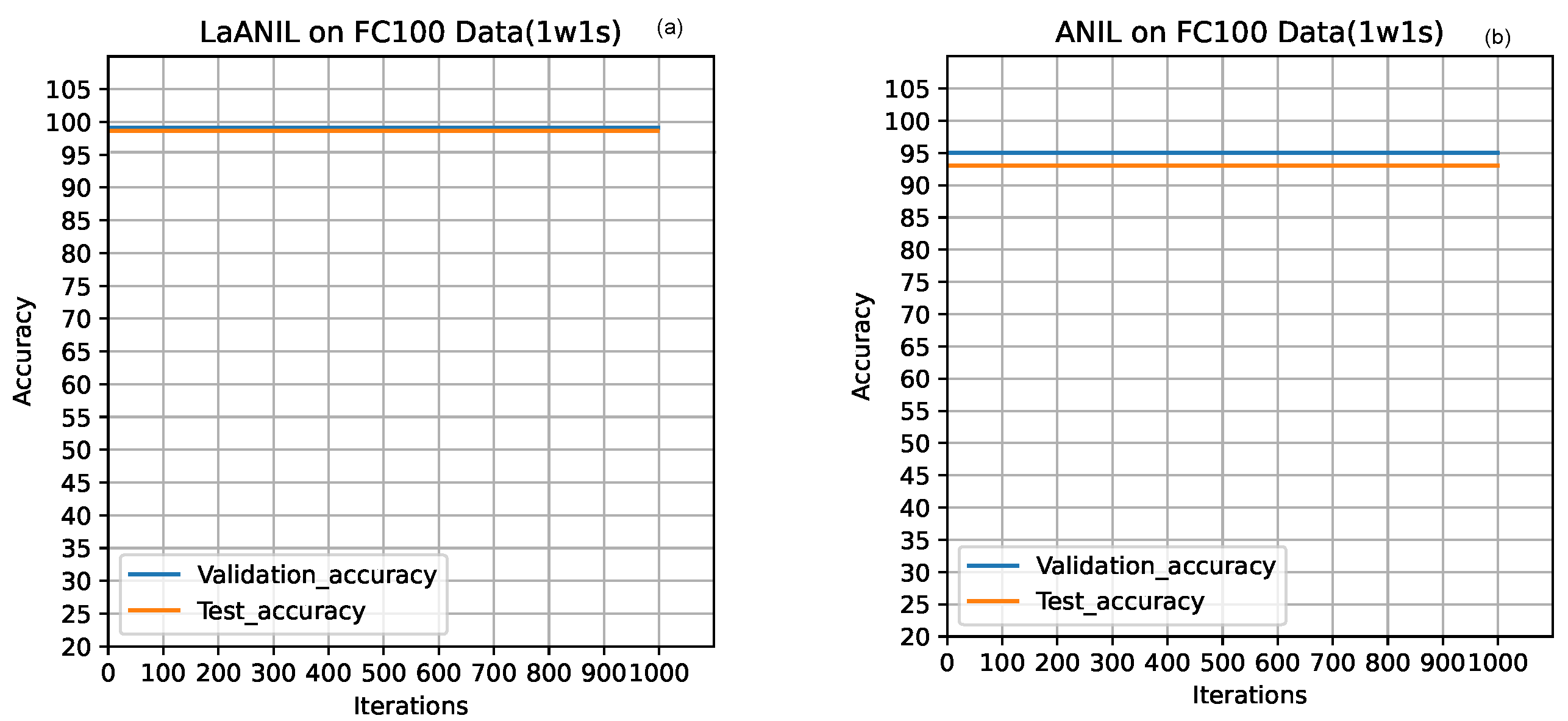
5.1. Rapid Adaptation

The rapid adaptability of LaANIL, as shown in Figure 8a,c,e and Figure 9a,c, is an advantageous aspect of our model compared to other models (see Tables 1, 5 and 6). The limited availability of labeled data often impedes meta-few-shot learning, yet LaANIL’s ability to adapt effectively is evident from the test accuracy results in Figure 8a,c,e and Figure 9c and

Table 1. Meta-few-shot image classification of ANIL vs. LaANIL for 1-way 1-shot (no variance observed in results for 1-way 1-shot classification).

Sno	Dataset	Base Model Validation Accuracy (ANIL)	Our Model Validation Accuracy (LaANIL)
1	FC-100%	95%	98%
2	CIFAR-FS	93%	95%
3	Mini-ImageNet	96%	99%
4	CUBirds-200-2011	95%	99%
5	Tiered-ImageNet	98%	99%

,

Table 2. Meta-few-shot image classification of ANIL vs. LaANIL for 2-way 2-shot.

Sno	Dataset	Base Model Validation Accuracy (ANIL)	Our Model LaANIL Validation Accuracy	Varience ANIL	Varience LaANIL
1	FC-100	71%	78%	21 ± 3%	6 ± 1%
2	CIFAR-FS	63%	68%	21.6 ± 3%	5 ± 1%
3	Mini-ImageNet	65%	72%	20 ± 2%	5 ± 1%
4	CUBirds-200-2011	66%	74%	23 ± 2%	7 ± 1%
5	Tiered-ImageNet	64%	73%	25 ± 4%	8 ± 1%

,

Table 3. Meta-few-shot image classification of ANIL vs. LaANIL for 5-way 5-shot.

Sno	Dataset	Base Model Validation Accuracy (ANIL)	Our Model LaANIL Validation Accuracy	Varience ANIL	Varience LaANIL
1	FC-100	47%	52%	15 ± 1%	4 ± 0.7%
2	CIFAR-FS	58%	62%	13 ± 1.5%	4 ± 0.8%
3	Mini-ImageNet	59%	63%	14 ± 1%	3 ± 0.5%
4	CUBirds-200-2011	58%	63%	13 ± 1%	5 ± 0.9%
5	Tiered-ImageNet	63%	66%	15 ± 1.5%	6 ± 1%

and

Table 4. Meta-few-shot image classification of ANIL vs. LaANIL for 2-way 10-shot.

Sno	Dataset	Base Model Validation Accuracy (ANIL)	Our Model LaANIL Validation Accuracy	Varience ANIL	Varience LaANIL
1	FC-100	68%	72%	6 ± 0.5%	2 ± 0.4%
2	CIFAR-FS	64%	70%	4.6 ± 3%	2 ± 0.5%
3	Mini-ImageNet	63%	69%	7 ± 0.8%	3 ± 0.5%
4	CUBirds-200-2011	66%	73%	8 ± 1%	2 ± 0.6%
5	Tiered-ImageNet	68%	72%	8 ± 1%	2.5 ± 0.7%

). The model’s adapting capability to new tasks compared to the base and other models mentioned in Table 1,

Table 5. Meta-few-shot image classification of different models and backbones on 5-way 5-shot.

Dataset	Model	Back Bone	Test Accuracy	Validation Accuracy	Varience (Validation)
mini ImageNet (5W5S)	ANIL	VGG	61.7 ± 1.77%	59.3 ± 2.27%	±17.5%
		CNN4	62.7 ± 1.87%	59.0 ± 1.97%	±14.5%
		ResNet12	62.7 ± 0.87%	59.3 ± 1.57%	±15.7%
	MAML	VGG	61.2 ± 1.1%	58.3 ± 2.17%	±17.5%
		CNN4	62.8 ± 1.87%	60.0 ± 1.35%	±13.3%
		ResNet12	63.16 ± 0.47%	60.5 ± 1.27%	±15.2%
	ProtoNet	VGG	61.5 ± 1.1%	59.3 ± 2.17%	±14.5%
		CNN4	62.0 ± 2.57%	60.0 ± 1.37%	±13.8%
		ResNet12	63.5 ± 0.77%	61.3 ± 1.57%	±18.1%
	LaANIL	VGG	62.5 ± 1.27%	62.3 ± 1.77%	±6.5%
		CNN4	65.2 ± 0.57%	64.3 ± 0.67%	±3.8%
		ResNet12	64.8 ± 0.87%	63.3 ± 1.17%	±5.5%

and

Table 6. Meta-few-shot image classification of different models and backbones for 2-way 2-shot.

Dataset	Model	Back Bone	Test Accuracy	Validation Accuracy	Varience (Validation)
Tiered ImageNet (2W2S)	ANIL	VGG	73.7 ± 1.77%	68.3 ± 1.2%	±22.1%
		CNN4	77.7 ± 1.87%	71.0 ± 1.37%	±21.5%
		ResNet12	78.7 ± 0.87%	70.3 ± 1.27%	±21.7%
	MAML	VGG	80.2 ± 1.1%	70.3 ± 2.17%	±30.5%
		CNN4	82.8 ± 1.87%	73.0 ± 1.25%	±28.3%
		ResNet12	83 ± 1.47%	74.5 ± 1.27%	±33.2%
	ProtoNet	VGG	79.5 ± 1.13%	72 ± 2.17%	±28.5%
		CNN4	82.0 ± 1.57%	71.0 ± 1.37%	±23.8%
		ResNet12	82.5 ± 0.77%	70.5 ± 1.57%	±21.1%
	LaANIL	VGG	80.5 ± 0.87%	74.3 ± 1.16%	±7.5%
		CNN4	84.2 ± 0.57%	78.3 ±0.67%	±6.1%
		ResNet12	84.8 ± 1.27%	73.6 ± 1.17%	±7.7%

can enhance its effectiveness in dynamic environments with frequent task changes.

This rapid adaptation is due to the parallel input processing and Nesterov’s momentum with adaptable learning rate capability. These methods allow the model to effectively utilize the information provided in the support set, thus diminishing the need for extensive data and computation. Nesterov’s momentum expedites the model’s convergence during training, further accelerating the adaptation process. In practical terms, LaANIL proves useful in rapidly developing and evolving scenarios, such as autonomous driving and computer vision endeavors for classification tasks. LaANIL’s ability to adapt quickly to new circumstances is a valuable asset for real-time decision-making compared to other models.

5.2. Better Generalization

These experiments yield improved model generalization, a crucial aspect of machine learning, whereby our model demonstrates proficiency in performing well on unobserved data relative to the other models like MAML, ProtoNet, and base-model ANIL (see Table 2 and Table 3).

The enhanced generalization observed in LaANIL (see the validation accuracy results in Figure 8a,c,e and Figure 9c) is a product of incorporating new methods into the base model. These methods allow the model to focus on relevant information in the support set, leading to improved generalization for new tasks. Additionally, incorporating Nesterov momentum and $L2$ regularization improves loss calculation. It helps refine the model’s weights through Nesterov’s momentum gradient descent while training and makes training more challenging for the model rather than just memorizing the data to avoid overfitting, resulting in enhanced generalization of the proposed model compared to different models with varying backbones (see Table 2 and Table 3). These findings are significant because they suggest that LaANIL has great potential to excel in scenarios where adaptation to unfamiliar categories is necessary. This is a critical aspect across various fields, such as image recognition and natural language processing, where the capacity to learn from a limited number of examples is important.

5.3. Low Variance

One notable result of LaANIL was the model’s minimal observed variance in performance in relation to MAML, ProtoNet, and base-model ANIL, as reported in the validation and test accuracy results of LaANIL vs. ANIL and other models in Figure 8 and Figure 9 and Table 2, Table 3, Table 4, Table 5 and Table 6.

In machine learning, variance refers to the fluctuations in prediction accuracy across multiple training runs or data splits. In the context of meta-few-shot learning, low variance is a crucial indicator of model stability. When a model exhibits low variance, it performs consistently well across various meta-few-shot tasks and data distributions. The implementation of Nesterov’s momentum and data parallelism in LaANIL has resulted in reduced variance and a more stable training process, providing significant advantages in real-world applications where consistent performance is essential. We can rely on LaANIL to consistently achieve high accuracy in meta-few-shot learning tasks. This is particularly advantageous in scenarios with constrained or rapidly changing data.

The differences in performance between our LaANIL model and the earlier model are illustrated in the graphs and tables presented. Notably, our model delivers exceptionally precise predictions with minimal variance [41], a vital characteristic in the field of meta-learning. These findings demonstrate the effectiveness of our methodology in overcoming obstacles associated with meta-few-shot learning in comparison to other models mentioned in this work and demonstrate its potential for broader application in the field. Our method enables models to learn from a small number of examples by optimizing their initial parameters for faster adaptation. The overall efficiency of the model is established against the base-model ANIL and others through validation on major meta-few-shot learning datasets, including FC100 CIFAR-FS, Mini-ImageNet, CUBirds-200-2011, and Tiered-ImageNet. Our approach empowers models to quickly adapt to new tasks with limited data, enhancing their ability to apply knowledge gained from prior experiences to novel scenarios, a crucial objective in modern machine learning research.

Overall, data parallelism and Nesterov’s momentum lead to improved regularization, generalization, and faster convergence of our model compared to the ANIL base model. Data parallelism increases diversity by training model copies on various data subsets, while Nesterov’s momentum modifies the momentum term for optimal gradient updates and optimization.

5.4. Edge Compatibility of New Model

Our model performed effectively on edge devices with restricted resources, such as Jetson Nano and Raspberry Pi, during training and testing on the mentioned datasets. As far as we know, ours is the first LaANIL and ANIL implementation on edge devices (see Figure 10). Data parallelism in LaANIL allows edge devices to divide training data proficiently, improving the pace of training and generalization ability (refer to Section 3 and Figure 3 and Figure 4) of the new model compared to MAML, ProtoNet, and base-model ANIL tested in this work. Our model worked well on edge devices with a minimum of 2GB RAM with or without GPU support. Moreover, Nesterov’s momentum enhances robustness, generalization, and convergence speed, all of which are imperative for the attainment of successful meta-few-shot learning on restrained edge devices [42]. The combination of these techniques can immensely benefit edge devices in overcoming meta-few-shot learning obstacles.

5.5. Ablation Studies

The model’s ability was studied using different combinations of new optimizer and data parallelism with two different backbones: CNN4 (our choice) and ResNet12. The results are shown in Figure 11. We primarily verified the model on its variance and validation accuracy, which are indications of rapid adaptability of the model essential in meta-few-shot learning. From the ablation studies (Figure 11), we observed low accuracy and high variance in all cases when Nesterov’s momentum and data parallelism were excluded. However, when we gradually introduced new methods, there was an improvement in validation accuracy and a reduction in variance. High variance can lead to low confidence in predictions. Based on Figure 11, it can be concluded that our proposal effectively addresses the issues of the base model. Furthermore, our new methods have been shown to work effectively on different models with varying backbone feature extractors.

6. Conclusions

Meta-few-shot image classification, a task within the field of meta-learning, holds significant promise in enabling machines to quickly master complex tasks with minimal data. This approach reduces the need for the laborious data gathering necessary for model development. ANIL is a meta-learning algorithm that features a streamlined architecture and inherent computational advantages over MAML, yet it encounters substantial challenges in flexibility and generalization, including the handling of diverse data types, the adaptation to new scenarios with limited data, and the transfer of knowledge across domains.

In this work, we introduced LaANIL, an updated algorithmic approach aimed at overcoming deficiencies and increasing the effectiveness of ANIL in real-world scenarios. By reorganizing ANIL’s internal architecture, integrating parallel computing techniques, and incorporating Nesterov’s momentum for optimized look-ahead gradient calculations, this stabilization technique amplifies the model’s ability to adapt quickly in dynamic environments.

LaANIL has been evaluated on a variety of meta-few-shot learning benchmark datasets, including FC100 CIFAR-FS, Mini-ImageNet, CUBirds-200-2011, and Tiered-ImageNet.

More generally, this study presented recent meta-learning advancements as a means of reducing the vast disparity between human and machine learning speeds while addressing conventional deep learning limitations. Notably, the results show positive performance in meta-few-shot classification utilizing just one to ten examples per category. However, as the number of categories increases, the model experiences issues such as high loss and low accuracy. Additionally, the training effectiveness of LaANIL heavily relies on the selection of meta-features and hyperparameters, which can be challenging to determine within a limited time frame. Utilizing inventive and efficient approaches for selecting and optimizing hyperparameters could improve LaANIL’s learning efficiency, making it more appropriate for real-world applications such as object detection. Additionally, enhancing the efficiency of loss functions and hybrid optimization algorithms with an ensemble strategy has the potential to enhance classification accuracy and decrease the computational requirements during LaANIL’s training.

References

1. Khan, I.; Zhang, X.; Rehman, M.; Ali, R. A literature survey and empirical study of meta-learning for classifier selection. IEEE Access 2020, 8, 10262–10281. [Google Scholar] [CrossRef]
2. Chen, Y.; Liu, Z.; Xu, H.; Darrell, T.; Wang, X. Meta-Baseline: Exploring Simple Meta-Learning for Few-Shot Learning. In Proceedings of the IEEE/CVF International Conference on Computer Vision (ICCV), Montreal, BC, Canada, 11–17 October 2021; pp. 9062–9071. [Google Scholar]
3. Finn, C.; Abbeel, P.; Levine, S. Model-agnostic meta-learning for fast adaptation of deep networks. In Proceedings of the International Conference on Machine Learning, PMLR, Sydney, NSW, Australia, 6–11 August 2017; pp. 1126–1135. [Google Scholar]
4. Raghu, A.; Raghu, M.; Bengio, S.; Vinyals, O. Rapid learning or feature reuse? Towards understanding the effectiveness of maml. arXiv 2019, arXiv:1909.09157. [Google Scholar]
5. Tian, P.; Li, W.; Gao, Y. Consistent meta-regularization for better meta-knowledge in few-shot learning. IEEE Trans. Neural Netw. Learn. Syst. 2021, 33, 7277–7288. [Google Scholar] [CrossRef] [PubMed]
6. Fan, Y.; Zhang, J.; Zhao, N.; Ren, Y.; Wan, J.; Zhou, L.; Shen, Z.; Wang, J.; Zhang, J.; Wei, Z. Model aggregation method for data parallelism in distributed real-time machine learning of smart sensing equipment. IEEE Access 2019, 7, 172065–172073. [Google Scholar] [CrossRef]
7. Sun, C.M.; Chen, Z.; Lin, L. Counterfactual Balancing Feature Alignment for Few-Shot Cross-Domain Scene Parsing. IEEE Access 2023. [Google Scholar] [CrossRef]
8. Zhao, S.; Li, F.; Chen, X.; Guan, X.; Jiang, J.; Huang, D.; Qing, Y.; Wang, S.; Wang, P.; Zhang, G.; et al. vpipe: A virtualized acceleration system for achieving efficient and scalable pipeline parallel dnn training. IEEE Trans. Parallel Distrib. Syst. 2021, 33, 489–506. [Google Scholar] [CrossRef]
9. Goddard, H.; Shamir, L. SVMnet: Non-Parametric Image Classification Based on Convolutional Ensembles of Support Vector Machines for Small Training Sets. IEEE Access 2022, 10, 24029–24038. [Google Scholar] [CrossRef]
10. Gu, P.; Tian, S.; Chen, Y. Iterative learning control based on Nesterov accelerated gradient method. IEEE Access 2019, 7, 115836–115842. [Google Scholar] [CrossRef]
11. Chen, X.W.; Lin, X. Big data deep learning: Challenges and perspectives. IEEE Access 2014, 2, 514–525. [Google Scholar] [CrossRef]
12. Luo, X.; Xu, J.; Xu, Z. Channel Importance Matters in Few-Shot Image Classification. In Proceedings of the 39th International Conference on Machine Learning, PMLR, Baltimore, MD, USA, 17–23 July 2022; Chaudhuri, K., Jegelka, S., Song, L., Szepesvari, C., Niu, G., Sabato, S., Eds.; Proceedings of Machine Learning Research: New York, NY, USA, 2022; Volume 162, pp. 14542–14559. [Google Scholar]
13. Hutter, F.; Kotthoff, L.; Vanschoren, J. Automated Machine Learning: Methods, Systems, Challenges; Springer Nature: Berlin/Heidelberg, Germany, 2019. [Google Scholar]
14. Tian, Y.; Zhao, X.; Huang, W. Meta-learning approaches for learning-to-learn in deep learning: A survey. Neurocomputing 2022, 494, 203–223. [Google Scholar] [CrossRef]
15. Lee, T.; Yoo, S. Augmenting few-shot learning with supervised contrastive learning. IEEE Access 2021, 9, 61466–61474. [Google Scholar] [CrossRef]
16. Wang, Y.; Gui, G.; Lin, Y.; Wu, H.C.; Yuen, C.; Adachi, F. Few-shot specific emitter identification via deep metric ensemble learning. IEEE Internet Things J. 2022, 9, 24980–24994. [Google Scholar] [CrossRef]
17. Fu, K.; Zhang, T.; Zhang, Y.; Yan, M.; Chang, Z.; Zhang, Z.; Sun, X. Meta-SSD: Towards fast adaptation for few-shot object detection with meta-learning. IEEE Access 2019, 7, 77597–77606. [Google Scholar] [CrossRef]
18. Lu, S.; Cui, X.; Squillante, M.S.; Kingsbury, B.; Horesh, L. Decentralized bilevel optimization for personalized client learning. In Proceedings of the ICASSP 2022-2022 IEEE International Conference on Acoustics, Speech and Signal Processing (ICASSP), Singapore, 23–27 May 2022; pp. 5543–5547. [Google Scholar]
19. He, Y.; Luo, F.; Ranzi, G. Transferrable model-agnostic meta-learning for short-term household load forecasting with limited training data. IEEE Trans. Power Syst. 2022, 37, 3177–3180. [Google Scholar] [CrossRef]
20. Chua, K.; Lei, Q.; Lee, J.D. How fine-tuning allows for effective meta-learning. In Proceedings of the Advances in Neural Information Processing Systems, Virtual, 6–14 December 2021; Volume 34, pp. 8871–8884. [Google Scholar]
21. Wu, M.; Jiang, F.; Liu, J.; Peng, Y. Application of C1DAE-ANIL in End-to-End Communication of IRS-Assisted UAV System. IEEE Access 2022, 10, 80703–80713. [Google Scholar] [CrossRef]
22. Collins, L.; Mokhtari, A.; Oh, S.; Shakkottai, S. Maml and anil provably learn representations. In Proceedings of the International Conference on Machine Learning, PMLR, Baltimore, MD, USA, 17–23 July 2022; pp. 4238–4310. [Google Scholar]
23. Miller, S.S.; Mocanu, P.T. Second order differential inequalities in the complex plane. J. Math. Anal. Appl. 1978, 65, 289–305. [Google Scholar] [CrossRef]
24. Sun, S.; Cao, Z.; Zhu, H.; Zhao, J. A survey of optimization methods from a machine learning perspective. IEEE Trans. Cybern. 2019, 50, 3668–3681. [Google Scholar] [CrossRef] [PubMed]
25. Aimen, A.; Sidheekh, S.; Madan, V.; Krishnan, N.C. Stress testing of meta-learning approaches for few-shot learning. In Proceedings of the AAAI Workshop on Meta-Learning and MetaDL Challenge, PMLR, Virtual, 9 February 2021; pp. 38–44. [Google Scholar]
26. Fan, Q.; Peng, J.; Li, H.; Lin, S. Convergence of a gradient-based learning algorithm with penalty for ridge polynomial neural networks. IEEE Access 2020, 9, 28742–28752. [Google Scholar] [CrossRef]
27. Wang, B.; Wang, D. Plant leaves classification: A few-shot learning method based on siamese network. IEEE Access 2019, 7, 151754–151763. [Google Scholar] [CrossRef]
28. Zhao, Y.; Gao, X.; Shumailov, I.; Fusi, N.; Mullins, R. Rapid Model Architecture Adaption for Meta-Learning. In Proceedings of the Advances in Neural Information Processing Systems, New Orleans, LA, USA, 28 November–9 December 2022; Volume 35, pp. 18721–18732. [Google Scholar]
29. Ye, H.J.; Sheng, X.R.; Zhan, D.C. Few-shot learning with adaptively initialized task optimizer: A practical meta-learning approach. Mach. Learn. 2020, 109, 643–664. [Google Scholar] [CrossRef]
30. Chen, M. Analysis of Data Parallelism Methods with Deep Neural Network. In Proceedings of the 2022 6th International Conference on Electronic Information Technology and Computer Engineering, Xiamen, China, 21–23 October 2022; pp. 1857–1861. [Google Scholar]
31. Tang, S.; Shen, C.; Wang, D.; Li, S.; Huang, W.; Zhu, Z. Adaptive deep feature learning network with Nesterov momentum and its application to rotating machinery fault diagnosis. Neurocomputing 2018, 305, 1–14. [Google Scholar] [CrossRef]
32. Dozat, T. Incorporating Nesterov Momentum into Adam. In Proceedings of the ICLR 2016 Workshop, San Juan, Puerto Rico, 2–4 May 2016. [Google Scholar]
33. Zaheer, M.; Reddi, S.; Sachan, D.; Kale, S.; Kumar, S. Adaptive methods for nonconvex optimization. In Proceedings of the Advances in Neural Information Processing Systems, Montréal, QC, Canada, 3–8 December 2018; Volume 31. [Google Scholar]
34. Xiao, B.; Liu, Y.; Xiao, B. Accurate state-of-charge estimation approach for lithium-ion batteries by gated recurrent unit with ensemble optimizer. IEEE Access 2019, 7, 54192–54202. [Google Scholar] [CrossRef]
35. Korkmaz, E. Nesterov momentum adversarial perturbations in the deep reinforcement learning domain. In Proceedings of the International Conference on Machine Learning, ICML, Virtual, 13–18 July 2020. [Google Scholar]
36. Hashemi, S.R.; Salehi, S.S.M.; Erdogmus, D.; Prabhu, S.P.; Warfield, S.K.; Gholipour, A. Asymmetric loss functions and deep densely-connected networks for highly-imbalanced medical image segmentation: Application to multiple sclerosis lesion detection. IEEE Access 2018, 7, 1721–1735. [Google Scholar] [CrossRef]
37. Khan, M.U.; Jawad, M.; Khan, S.U. Adadb: Adaptive diff-batch optimization technique for gradient descent. IEEE Access 2021, 9, 99581–99588. [Google Scholar] [CrossRef]
38. Jamal, M.A.; Qi, G.J. Task agnostic meta-learning for few-shot learning. In Proceedings of the IEEE/CVF Conference on Computer Vision and Pattern Recognition, Long Beach, CA, USA, 15–20 June 2019; pp. 11719–11727. [Google Scholar]
39. Patowary, G.; Agarwalla, M.; Agarwal, S.; Sarma, M.P. A lightweight CNN architecture for land classification on satellite images. In Proceedings of the 2020 International Conference on Computational Performance Evaluation (ComPE), Shillong, India, 2–4 July 2020; pp. 362–366. [Google Scholar]
40. Karami, A.; Crawford, M.; Delp, E.J. Automatic plant counting and location based on a few-shot learning technique. IEEE J. Sel. Top. Appl. Earth Obs. Remote. Sens. 2020, 13, 5872–5886. [Google Scholar] [CrossRef]
41. Zhang, Z.; Wang, Y.; Liu, X. Tapnet: Enhancing trajectory prediction with auxiliary past learning task. In Proceedings of the 2021 IEEE Intelligent Vehicles Symposium (IV), Nagoya, Japan, 11–17 July 2021; pp. 421–426. [Google Scholar]
42. Mauro, G.; Chmurski, M.; Servadei, L.; Pegalajar-Cuellar, M.; Morales-Santos, D.P. Few-shot user-definable radar-based hand gesture recognition at the edge. IEEE Access 2022, 10, 29741–29759. [Google Scholar] [CrossRef]
Figure 1. Illustration of the computations of the ANIL (b) and MAML (a) algorithms. The crucial difference between MAML (a) and ANIL (b) lies in the fact that in MAML (a), all parameters initialized with the meta-initialization from the outer loop are subject to task-specific gradient updates from the inner loop. Conversely, when training and testing ANIL (b), the inner loop solely modifies the parameters corresponding to the network head.
Electronics 13 01585 g001
Figure 2. Paradigms of rapid learning (a) and feature reuse (b). In rapid learning, training in the outer loop produces parameter settings that facilitate fast learning, while updates in the inner loop result in significant task specialization. In feature reuse, the outer loop generates reusable feature-specific parameter values that do not significantly change in the inner loop.
Electronics 13 01585 g002
Figure 3. Forward pass of data using parallel computing and calculating Nesterov’s gradient. For simplicity, only three computing units are depicted.
Electronics 13 01585 g003
Figure 4. Backward pass of data using parallel computing and calculating Nesterov’s gradient.
Electronics 13 01585 g004
Figure 5. In section (a), standard gradient update; in (b), Nesterov’s momentum achieves stronger convergence by applying the velocity ( ν t ) to the parameters to compute interim parameters ( θ = θ t + μ ν t ) , where μ is the decay rate. These interim parameters are then used to compute the gradient, called a “look-ahead” gradient step or a Nesterov accelerated gradient.
Electronics 13 01585 g005
Figure 6. An example of 4-shot 2-way classification data split (images are from GitHub—https://uvadlc-notebooks.readthedocs.io/en/latest/tutorial_notebooks/tutorial16/Meta_Learning.html, accessed on 1 July 2023). For each class, we have 4 images, and we have to classify 2 types of images each time.
Electronics 13 01585 g006
Figure 7. Mean, mode and median distribution and skewness. (a) Left-skewed, (b) Normal distribution, (c) Right-Skewed.
Electronics 13 01585 g007
Figure 8. Some results of LaANIL vs. ANIL on FC100 data set. Parts (a,c,e) of the image show the results of the new model, and Parts (b,d,f) of the image show the results of the base model.
Electronics 13 01585 g008aElectronics 13 01585 g008b
Figure 9. Some results of LaANIL vs. ANIL on CIFASFS data. Parts (a,c) of the image show the results of the new model, and Parts (b,d) of the image show the results of the base model set.
Electronics 13 01585 g009
Figure 10. LaANIL’s performance on Jetson Nano (2w2s).
Electronics 13 01585 g010
Figure 11. Ablation studies of LaANIL with divergent combinations of different modules and backbones (a,b) with CNN4 as a backbone on FC100 data and (c,d) with ResNet12 as a backbone on Mini-imageNet.
Electronics 13 01585 g011