An LDPC-RS Concatenation and Decoding Scheme to Lower the Error Floor for FTN Signaling

Abstract

Faster-than-Nyquist (FTN) signaling has attracted increasing interest in the past two decades. However, when the fifth-generation (5G) communication low-density parity check (LDPC) code is applied to FTN signaling with low Bahl–Cock–Jelinek–Raviv (BCJR) states of detection and few turbo equalization iterations, an error floor near ${10}^{-5}$ is found, which does not exist in the original LDPC used for orthogonal signaling. This can be eliminated through many detection and decoding iterations, but this is unacceptable considering the increase in latency and storage. To solve this problem, we propose an LDPC and Reed–Solomon (RS) concatenation code, shortening, and perturbation scheme to lower the error floor. We propose a parallel encoder architecture for RS component code and a concise algorithm to calculate its constant multiplier coefficients, leveraging a traditional serial encoder, which can also be used for other parallelisms, rates, and lengths. The simulation results show that the proposed concatenation and shortening scheme can lower the error floor to about ${10}^{-7}$. The proposed scheme has an error correction capability for coded FTN signaling and successfully lowers the error floor with the limitation of few turbo iterations and few BCJR states.

1. Introduction

Faster-than-Nyquist (FTN) signaling dates back to the 1970s and has attracted increasing interest in the past two decades due to the lack of research into frequency resources and bandwidth in digital communication, such as wireless communication, satellite communication, and optical communication [1]. One common method to improve link capacity and spectrum efficiency (SE) is to adopt high-order modulation in an orthogonal (Nyquist) modulation scheme, for example, by using quadrature amplitude modulation (QAM), such as 16-QAM, 64-QAM, or even 4096-QAM. However, high-order modulation formats often require higher power and sensitivity on radio frequency (RF) devices. Moreover, a higher modulation order is more likely to suffer from noise since constellation symbols converging in 256-QAM compared to 16-QAM and requires improved linearity of RF devices, thus being a challenge for symbol recovery and decisions. Another attractive method is to use a lower modulation order but non-orthogonal modulation scheme, i.e., FTN signaling. By accelerating the symbol speed of transmission with a faster-than-Nyquist speed of no inter-symbol interference (ISI), controlled ISI and colored noise are introduced after match filtering, and they can be eliminated in many ways, such as with a whitening filter, orthogonal basis model (OBM), precoding, turbo equalizer, or Bahl–Cock–Jelinek–Raviv (BCJR) detector [2]. In band-limited scenarios like high-speed optical, wireless, and satellite communication, FTN signaling provides higher SE with the same modulation order at the price of a higher symbol rate (higher sampling rate) and additional digital signal processing to mitigate ISI [3].

In recent years, many ISI mitigation methods have been studied, including linear equalization, decision feedback equalization (DFE), frequency domain equalization at the receiver side, and precoding and pre-equalization at the transmitter side. Although these methods are relatively simple, their performance will degrade with severe ISI when applying the high-acceleration factor of FTN signaling. The BCJR algorithm performs trellis searching to find survivors and make decisions for each bit. However, when dealing with a high modulation order or long ISI taps, BCJR detection requires considerable memory space to store a large number of states and routes in trellises, which increases exponentially with ISI length. To solve this problem, reduced-state M-BCJR detection was studied in [2], and the authors showed that only 3-state BCJR is required for FTN signaling with acceleration factor $\tau =0.5$. In a coded system with iterative decoding, we can apply FTN signaling as an internal ISI mechanism and use BCJR detection to generate soft decision bits, i.e., log likelihood ratio (LLR), and exchange LLRs among the BCJR detector and soft channel decoder, which is called turbo equalization. In this work, we applied the M-BCJR algorithm together with LDPC-RS concatenation code to form a coded FTN signaling scheme and mitigate ISI through turbo equalization.

LDPC code was first proposed by Gallager in 1962 [4]. Originally, the LDPC received little attention due to limited theoretical knowledge and computer processing capacity. Over the years, with the increasing improvement in relevant basic theories and the vigorous development of computer science and technology, researchers have devoted increasing effort to the study of LDPC code. LDPC code has become one of the most popular coding technologies and has been widely used in various communication systems, such as wireless, satellite, and fiber communication. With sufficient code length, LDPC code can approach the Shannon limit [5] and be capable of error correction at a low signal-to-noise ratio (SNR). Among soft decision-decoding methods, belief propagation (BP) is a promising decoding scheme for the LDPC and for other codes that need soft decisions and iterative decoding.

A typical bit error rate (BER) curve of channel coding resembles a waterfall, i.e., the BER drops sharply when the signal-to-noise ratio (SNR) increases. However, an error floor phenomenon can be found with many LDPC codes; when SNR increases, the BER does not decrease, or the curve flattens. According to [6], the error floor [7] is caused by sub-optimal iterative decoding [8], near-code words [9], and absorbing and trapping sets [10]. In some situations, the error floor can not be eliminated, and there are some methods to lower the error floor, for example, designing a large-girth parity matrix to optimize the code structure; using concatenation code, such as RS-LDPC [11] or DVB BCH-LDPC code [12] that utilizes RS or BCH as the outer code and the LDPC as the inner code; or manually introducing low-magnitude noise to message-passing decoders to lower the error floor. For some conditions, such noise can actually improve decoding performance [13]. This improvement, based on the effect of noise, is called stochastic resonance. We can refer to the introduction of such noise as perturbation. Perturbation decoders have exceptional performance and very low resource costs [14] and may prove superior to the existing techniques [15] in computer memory and data storage applications [16]. Details about stochastic resonance can be found in [17]. Note that the error floor may occur in a particular code and may not occur in another, and it is hard to predict whether it will occur. For example, the 5G LDPC (7680, 3840) code used in this study has no error floor in orthogonal (Nyquist) systems. However, when utilizing FTN signaling, we found an error floor in a rate-1/2 LDPC code masked from the 5G base graph “BG2”. This is probably caused by the decoder’s non-linearity, too few turbo iterations, improper loop gain or code rate, or a weakness in the masked base matrix structure. Since this phenomenon exists and is unpredictable, we require a method to lower the error floor that may occur in the demand region of the BER for practical situations. In this work, we utilized two of the above methods: LDPC-RS concatenated code and a perturbation BP decoder to lower the error floor.

Reed–Solomon (RS) code was invented by Reed and Solomon [18]. RS code has undergone decades of development and has been used in wireless, satellite, and optical communications due to its maximum distance separable (MDS) feature. A hard decision decoder is often utilized for high-speed or concatenated code due to its simple structure and high throughput. In this study, we used soft decision LDPC code due to its excellent error correction ability concatenated with hard decision RS code because of its high decoding speed and definite error correction ability.

Our contribution in this paper can be summarized in two points: (1) To combat the error floor, we propose one possible solution, the use of the LDPC-RS concatenation and shortening scheme. We introduce perturbation into the BP decoder to enhance its performance. (2) We propose a 4-parallel encoder architecture for RS component code and a concise algorithm to calculate its constant multiplier coefficients, leveraging a traditional serial encoder, which can also be used for calculating other parallelisms, code rates, and lengths. The simulation results show that the proposed concatenation and shortening scheme can lower the error floor of the original single LDPC code, and with perturbation in the BP decoder, the error floor can be eliminated below ${10}^{-7}$ for different LDPC maximum decoding iterations. The proposed scheme has an error correction ability for BCJR detection with few states and few iterations of turbo equalization FTN signaling and successfully lowers the error floor.

The outline of this paper is as follows: Section 2 reviews preliminaries of FTN signaling with the OBM, BCJR detection, turbo equalization, LDPC, and RS codes, as well as our simulations with 5G LDPC code and an error floor. Section 3 details the structure of the proposed LDPC-RS concatenation code, RS parallel RS encoder and algorithm for parallel encoding coefficient calculation, and the perturbation BP decoder to lower the error floor. Section 4 describes the performed simulations and analysis. Section 5 concludes the paper.

2. FTN Signaling with Turbo Equalization

2.1. FTN Signaling with OBM

The concept of FTN signaling was introduced by Mazo [19] in 1975. In FTN signaling, binary $\mathrm{sinc}(t/T)$ pulses can be transmitted faster than typical orthogonal (Nyquist) pulses without decreasing the square of minimum Euclidean distance between symbols, thus theoretically not affecting the bit error rate (BER) of demodulation. The binary baseband modulation of FTN signaling is linear and based on pulse shaping as follows:

$$s\left(t\right)=\sqrt{E_b/T}\sum _n{a}_{n}h(t-n\tau T),$$

(1)

where $E_b$ is the average symbol energy, $a_n$ represents $\pm 1$, $h\left(t\right)$ is a T-orthogonal unit energy-shaping pulse filter such as sinc or root-raised-cosine (rRC), the symbol interval of $a_n$ is $\tau T$, the acceleration factor is $\tau \le 1$, and n is the symbol index. Regarding Nyquist signaling, $\tau =1$.

We use discrete-time ISI and the additive white Gaussian noise (AWGN) channel model in [2] as the following chain of signal processing.

Data $\left\{a_n\right\}$ at $n\tau T$→ linear modulation and pulse shaping by $h\left(t\right)$ at rate $1/\tau T$→ AWGN → matched filter → sample at $n\tau T\to$ discrete-time post filter $B\left(z\right)$→ frame reverse → channel observation $\mathit{y}$.

This chain produces a minimum phase sequence of channel observation $\mathit{y}$ and can be applied to turbo equalization as detailed in the next subsection. Furthermore, the orthogonal basis model (OBM) receiver uses a sequence of wider band orthogonal pulses to express $h\left(t\right)$ as follows:

$$h\left(t\right)=\sum _{k=-K}^K{c}_k\varphi (t-k\tau T),$$

(2)

$$c_k=\int h\left(t\right)\varphi (t-k\tau T)\mathrm{d}t.$$

(3)

It is worth mentioning that basis function $\varphi \left(t\right)$ is $\tau T$-orthogonal, and the matched filter is matched to $\varphi \left(t\right)$ rather than $h\left(t\right)$; thus, the noise it outputs is white, which solves the colored noise problem in other receivers. The signal processing chain can be modeled as discrete-time system $\mathit{v}$ such that

$$\mathit{y}=\mathit{a}\ast \mathit{v}+\mathit{w},$$

(4)

where $\mathit{a}=\left\{a_n\right\}$, ∗ means convolution, and $\mathit{w}$ is a vector of independent identical distribution (i.i.d.) white Gaussian noise.

Regarding $\tau =0.703$, we use $\mathit{v}$ = [0.553, 0.793, −0.084, −0.171, 0.154, −0.064, 0.006, 0.010, −0.012, 0.015, −0.016, 0.013, −0.008] in [2], which is shortened to reduce memory usage during the simulations to the following:

$$\mathit{v}=[0.553,0.793,-0.084,-0.171,0.154,-0.064].$$

(5)

Consequently, turbo equalization (the BCJR detector) utilizes a minimum phase model of ISI and white noise. The detector branch label l at trellis stage n is generated from data $\mathit{a}$ as follows:

$$l=\sum _{n=0}^m{a}_{n-k}{v}_k,$$

(6)

where m is the length of $\mathit{v}$ taken into account (which may be shortened due to memory limitations).

2.2. BCJR Detection and Turbo Equalization

The BCJR algorithm computes the probability of states and paths in trellises. It performs forward and backward recursion among the state transition map. Suppose the channel observation $\mathit{y}=y_1,y_2,\dots ,y_N$, and the a priori symbol probability of each transmitted symbol is known. The joint probability can therefore be calculated as follows:

$$P(s_n=i,s_{n+1}=j,\mathit{y})={\alpha }_n\left[i\right]{\mathrm{\Gamma }}_n(i,j){\beta }_{n+1}\left[j\right],$$

(7)

where ${\alpha }_n\left[i\right]$ is called the forward path metric for state i at stage n, ${\beta }_{n+1}\left[j\right]$ is called the backward path metric for state j at stage $n+1$, and ${\mathrm{\Gamma }}_n(i,j)$ is the branch metric connecting states i and j at stage n. Usually, the transmitted symbols start from (and terminate at) an initial all-zero state, so that

$${\alpha }_{n+1}\left[i\right]=\sum _{i\in S}{\alpha }_n\left[i\right]{\mathrm{\Gamma }}_n(i,j)$$

(8)

is initialized as ${\alpha }_0=(1,0,\dots ,0)$, where S is the set of states that can reach state j at stage $n+1$. Regarding binary modulation, there are two elements in set S. Backward recursion is similar in that ${\beta }_N=(1,0,\dots ,0)$. It starts from the last symbol (stage) then proceeds backward to the beginning, computing the backward path metric as follows:

$${\beta }_n\left[i\right]=\sum _{j\in S}{\beta }_{n+1}\left[i\right]{\mathrm{\Gamma }}_n(i,j)$$

(9)

where S is the set of states that can reach state i at stage n. The branch metric is

$${\mathrm{\Gamma }}_n\left[i\right]=[P\left(a^{\prime }\right)/\sqrt{\pi N_0}]\exp [-{(y_n-l_{i,j})}^2/N_0)],$$

(10)

where $l_{i,j}$ is a label on the branch from state i to j, and $P\left(a^{\prime }\right)$ is the a priori probability of symbol $a^{\prime }$, which causes the transition (from state i to j). Let ${\lambda }_n\left[j\right]={\alpha }_n\left[j\right]{\beta }_n\left[j\right]$, and let j be a state at stage n. Then, we calculate LLRs via

$$LLR\left(a_n\right)=ln\frac{\mathrm{P}[a_n=+1]}{\mathrm{P}[a_n=-1]}=ln\frac{{\sum }_{j\in {\mathcal{L}}_{+1}}{\lambda }_n\left[j\right]}{{\sum }_{j\in {\mathcal{L}}_{-1}}{\lambda }_n\left[j\right]},$$

(11)

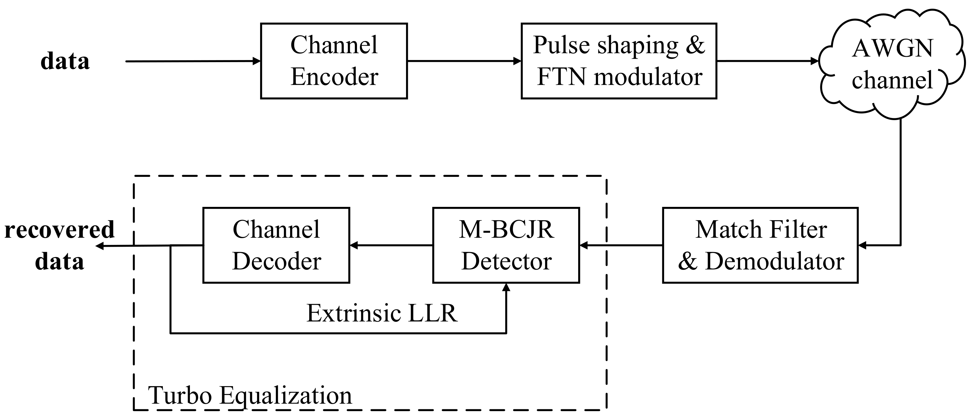
and ${\mathcal{L}}_{\pm 1}$ are sets of states reached by $a_n=\pm 1$. The M-BCJR algorithm proposed by [2] utilized the reduced search of trees and trellises. It proceeds breadth-first through a tree structure of metric values, keeping only the dominant M paths at each tree stage, and it also deals with empty values of ${\alpha }_n\left[j\right]$, ${\beta }_n\left[j\right]$. More details can be found in [2]. In coded FTN signaling, turbo equalization is usually adopted, whereby the BCJR detector and channel decoder exchange soft information iteratively. Turbo equalization enhances detector and decoder performance but increases complexity and latency proportional to turbo iterations. The coded FTN signaling diagram is depicted in Figure 1, where the dashed box represents turbo equalization.

2.3. LDPC and RS Code

Let N be the block length of the LDPC code and $\mathit{K}$ be the data length; then, $M=N-K$ is the parity length. Let $\mathit{d}=(d_1,d_2,\dots ,d_K)$ be the data and $\mathit{G}$ be the generation matrix of K-by-N size. The code word $\mathit{c}=\mathit{d}\mathit{G}$ has the property $\mathit{c}{\mathit{H}}^T=0$, where $\mathit{H}$ is the parity matrix of M-by-N. The code is called low-density parity check code, a feature of which is that parity matrix $\mathit{H}$ is sparse; namely, there are many zeros and few ones in $\mathit{H}$. There are binary and non-binary LDPC codes, and only binary codes are discussed in this work. LDPC codes can be classified into two types from the construction of parity matrix $\mathit{H}$, as regular and irregular codes. The number of ones in a row (column) of $\mathit{H}$ is called the row (column) degree. Regular codes have the same row degree for each row and the same column degree for each column. Row i’s degree indicates how many variable nodes are connected to check node i, and column j’s degree indicates how many check nodes are connected to variable node j. Among soft decision-decoding methods, belief propagation (BP) is a promising decoding scheme for the LDPC and other codes that need soft decisions and iterative decoding. The BP decoder uses message passing and iteration to propagate soft information among check and variable nodes. Since BP involves many nonlinear calculations, the min-sum (MS) algorithm was proposed. This algorithm uses the minimum value of soft information from relevant variable nodes to approximate the result of nonlinear functions that the BP decoder performs, thus reducing computation complexity and latency significantly [20]. Although the MS decoder requires fewer computations, the approximated results always have a greater absolute value than those of BP, which causes performance degradation. To mitigate performance loss, the normalized min-sum (NMS) scheme [21] and its variant were studied [22]; moreover, a neural network-aided NMS approach was proposed in [23]. The BP decoding scheme can be described as Algorithm 1.

Algorithm 1 BP Decoding of LDPC Code.

Define:     Set of variable nodes connected to check node i: $N\left(i\right)=\{j:h_{ij}=1\}$.     Set of check nodes connected to variable node j: $M\left(j\right)=\{i:h_{ij}=1\}$.     Soft information from variable node j to check node i: $Z_{ij}$.     Soft information from check node i to variable node j: $L_{ij}$. Input: Soft bit information: $\mathit{L}=(l_1,l_2,\dots ,l_n)$. Initialization: $Z_{ij}=l_j$. Iteration: For each $i,j$, the following steps are performed until the stopping criterion is satisfied.      (1) Row operation: For each check node i, calculate $$L_i=\prod _{j\in N\left(i\right)}tanh\left(\frac{Z_{ij}}{2}\right),$$ (12)      and for messages from i to each relevant variable node j, $$L_{ij}=2{tanh}^{-1}(L_i/tanh\left(\frac{Z_{ij}}{2}\right)).$$ (13)      (2) Column operation: For each variable node j, $$Z_j=l_j+\sum _{i\in M\left(j\right)}{L}_{ij},$$ (14)      and the message passed from j to each relevant check node i is $$Z_{ij}=Z_j-L_{ij}.$$ (15)      (3) Stopping criterion:      Make hard decision $\mathit{b}=(b_1,b_2,\dots ,b_n)$ from $Z_j$ as $$b_i=\left\{\begin{array}{ccc}0,\hfill & \mathrm{if}{Z}_j>0,\hfill & \mathrm{if}{Z}_j\le 0.\end{array}\right.$$ (16)      If ${\mathit{bH}}^T=\mathit{0}$ (no error) or the maximum iteration limit has been reached, stop the decoder, otherwise continue. Output: The decoding result $\mathit{b}$.

RS code is defined with finite field $\mathbb{GF}\left(2^p\right)$, where p is a positive integer, and all calculations are performed with this field. RS(n,k) code has code word length n and k data symbols, each symbol having p bits. It can correct up to $\lfloor (n-k)/2\rfloor$ errors. Let the data symbols be $\mathit{m}=(m_0,m_1,\dots ,m_{k-1})$ and be represented with polynomial $m\left(x\right)=m_0+m_{1}x+m_2{x}^2+\dots +m_{k-1}{x}^{k-1}$. Suppose the generator polynomial is $g\left(x\right)=(x-{\sigma }^1)(x-{\sigma }^2)\dots (x-{\sigma }^{n-k})=x^{(n-k)}+g_{n-k-1}{x}^{n-k-1}+\dots +g_{1}x+g_0$, where $\sigma$ is a prime element of $\mathbb{GF}\left(2^p\right)$. Then, the code word $\mathit{c}=(c_0,c_1,\dots ,c_{n-1})$ can be calculated as follows:

$$c\left(x\right)=x^{n-k}m\left(x\right)+x^{n-k}m\left(x\right)modg\left(x\right)=c_0+c_{1}x+\dots +c_{n-1}{x}^{n-1}.$$

(17)

2.4. Experiment with 5G LDPC Code and Turbo Equalization in FTN Signaling

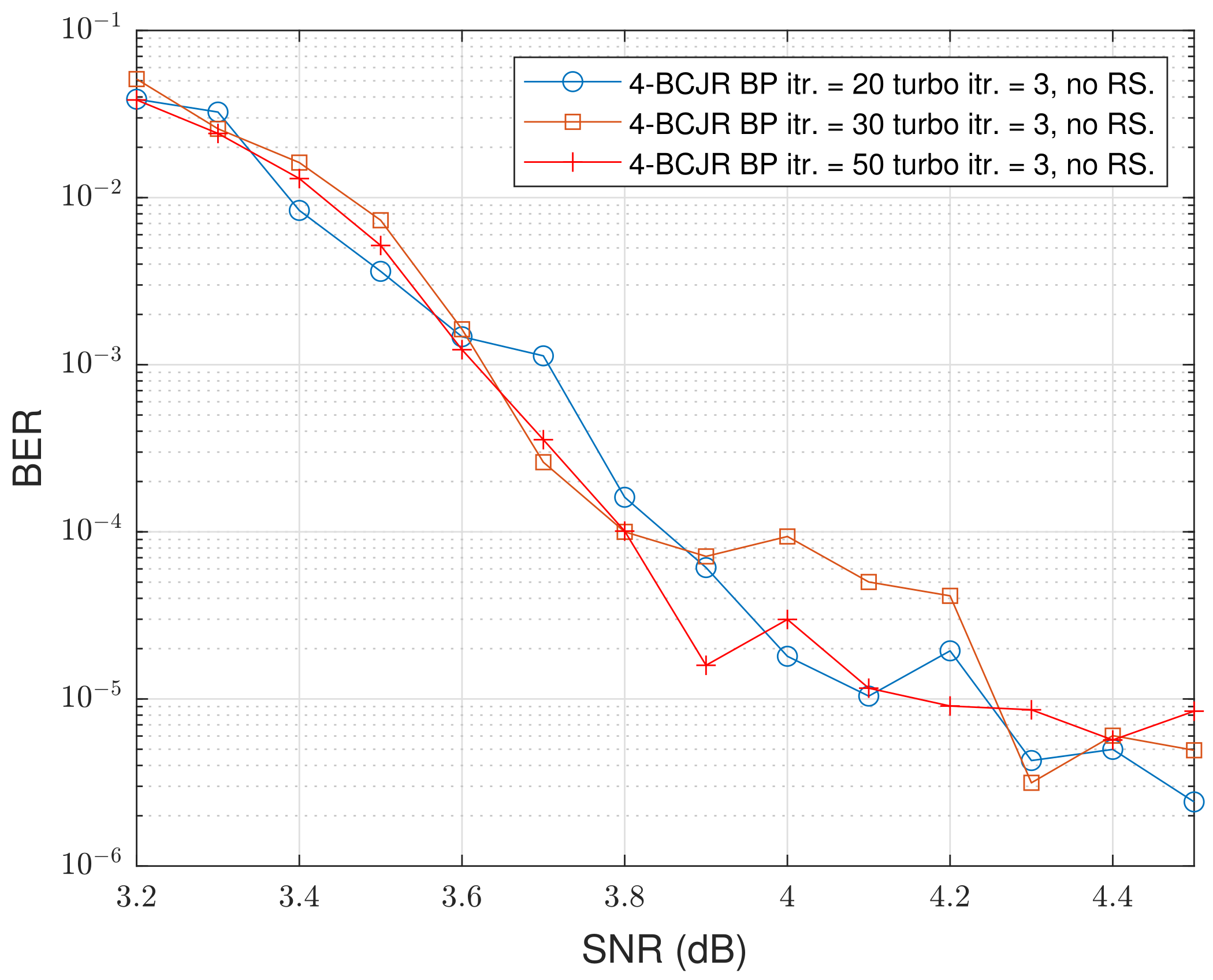
We simulated 5G LDPC code and turbo equalization in FTN signaling with MATLAB. The diagram is depicted in Figure 1. The LDPC code used here is a (7680, 3840) code based on BG2 [24]. We used shortened $\mathit{v}$ as in (5) and used BPSK modulation for the baseband system model. We used turbo equalization containing an M-BCJR detector and BP decoding for demodulation. Considering complexity and latency, we chose a maximum turbo equalization count of 3 to lower the number of whole iterations and $M=4$ states stored at each stage of the trellis in BCJR detection, i.e., 4-BCJR detection, to reduce memory usage. We considered maximum iteration limits of 10, 20, and 50 for BP decoding. Therefore, in total, three iterations of the 4-BCJR algorithm and 30, 60, and 150 iterations of BP decoding were performed at most for three turbo iterations. Unfortunately, an error floor was found near ${10}^{-5}$ as in Figure 2. It can be eliminated through many detection and decoding iterations, but this is unacceptable considering the low latency and storage. Accordingly, few turbo iterations and states of FTN detection can be adopted. With sufficient SNR, the error floor of the BP decoder will disappear independently. It appears in the BER region (${10}^{-5}$) of most concern in wireless communication, which is why we must lower or eliminate the error floor.

3. LDPC-RS Concatenation Code

3.1. Occurrence of an Error Floor in FTN Signaling

Inter-symbol interference caused by FTN signaling introduced relevance between symbols and code words. Additionally, shortening or tail cutting of the pulse-shaping filter and the channel response further complicate symbol relevance canceling. The LDPC code shows good performance with the AWGN channel, where symbols and noise are all independent. While applying FTN signaling and M-BCJR detection, there is residual relevance (interference) between symbols since we cannot accurately simulate an infinite pulse-shaping filter or channel response. On the other hand, LDPC code sometimes independently suffers from error propagation, stopping and trapping sets of its factor graph [17]. Thus, FTN signaling makes the LDPC code’s weakness obvious, and therefore an error floor occurs. The smaller the acceleration factor value is, the more severe the ISI that will occur, and thus, the BER performance of the LDPC will be poor, and the error floor will still occur.

The error floor is caused by FTN signaling and residual relevance (interference) between symbols. Since the M-BCJR algorithm is already a good detection scheme from the decoder perspective, we used shortening to provide some absolutely right bits of the LDPC—known bits with a high LLR in the factor graph in order to help the BP decoder partially overcome error propagation. Furthermore, we utilized perturbation to add low power noise to calculation of all check nodes during BP decoding. Since the operation is summation, confident nodes with high LLR values will not be affected, but those nodes of low reliability (a low magnitude of LLR) will be perturbed and may be corrected or move away from stopping or trapping sets, which are believed to be a reason for the error floor.

3.2. Structure of the Proposed LDPC-RS Concatenation Code

Typical concatenation code consists of inner and outer code. Data bits are encoded by the outer code, and the whole outer code word is treated as data that are part of the inner code; then, the inner encoder encodes it to form the inner (final) code word.

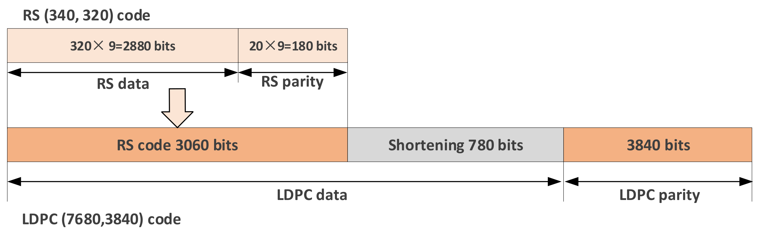
The structure of the proposed LDPC-RS concatenation code is depicted in Figure 3. We chose RS (340, 320) and a shortened version of RS (511, 491) code for BP decoding, and the corresponding generation polynomial coefficients are 1, 58, 257, 157, 222, 388, 151, 62, 280, 137, 404, 286, 394, 61, 399, 73, 84, 145, 293, 369, and 331. We adopted 5G LDPC (7680, 3840) code for the inner code, with 780 bits shortened (filled with a known pattern which is not transmitted) and accustomed to the 3060-bit length of outer RS (340, 320) code. Therefore, there are $320\times 9=2880$ bits of data, the total transmitted code length is $340\times 9+3840=6900$ bits, and the code rate is $2880/6900=0.4174$. The price of 0.09 rate-loss is acceptable considering rate and error floor trade-off.

3.3. Perturbation BP Decoder

One reason for the error floor is that the BP decoder cannot correct nodes for some code structures and absorbing sets, becoming trapped in incorrect states. One example of the (6, 3) trapping set is given in Figure 4, where all variable nodes $v_1,v_2,v_3$ are incorrect and where check nodes are too weak to correct them, so all three variable nodes remain erroneous. Finally, several uncorrected error bits can be corrected using concatenated RS code due to its definite error correction ability. When using a parallel RS encoder or decoder, latency and complexity can be lowered.

Moreover, the BP decoder will sometimes encounter errors with very few LLRs, while adding some low-level noise to the decoder can actually improve decoding performance. This phenomenon is called stochastic resonance and was found in many devices and research fields and studied using [25] for bit-flipping decoding. In this work, we adopted this method in the soft decision BP decoder, adding a low level of noise to nodes while decoding, and called it the perturbation BP decoder. We modified the message from check node i to each relevant variable node j by adding noise (perturbation) to affect or flip the signs of small absolute value LLRs, which are believed to be less reliable, as follows:

$$L_{ij}^{\prime }=2{tanh}^{-1}(L_i/tanh(\frac{Z_{ij}}{2}))+n_p,$$

(18)

where $n_p$ is low-level i.i.d. random noise, irrelevant to $i,j$, with the expectation that $E\left(n_p\right)=0$, and variance $\mathit{Var}\left(n_p\right)={\sigma }_{np}^2$ is irrelevant to $i,j$. Its power ${\sigma }_{np}^2$ can be chosen in practice, and its type was chosen to be Gaussian here; thus,

$$\begin{array}{cc}\hfill & E\left(L_{ij}^{\prime }\right)=E\left(L_{ij}\right),\hfill \\ \hfill & \mathit{Var}\left(L_{ij}^{\prime }\right)=\mathit{Var}\left(L_{ij}\right)+{\sigma }_{np}^2.\hfill \end{array}$$

(19)

Note that adding noise (perturbation) to LLRs is a more general form of adding the same offset value, which has been shown to be effective in a hard decision bit-flipping decoder. The perturbation decoder proposed here can be seen as a soft bit-flipping BP decoder. From a statistical viewpoint, it adds power ${\sigma }_{np}^2$ to LLRs of small absolute value.

Since $E\left(n_p\right)=0$, the summation of i.i.d. random Gaussian noise will tend toward a small value near zero, so for variable node j, the updating rule becomes

$$Z_j^{\prime }=l_j+\sum _{i\in M\left(j\right)}{L}_{ij}^{\prime }\approx l_j+\sum _{i\in M\left(j\right)}{L}_{ij}=Z_j,$$

(20)

and the message passed from variable node j to each relevant check node i is

$$Z_{ij}^{\prime }=Z_j^{\prime }-L_{ij}^{\prime }\approx Z_{ij}.$$

(21)

Therefore, perturbation here only affects unreliable check nodes with very small absolute value $L_{ij}$, making them perturbed. The histogram in Figure 5 illustrates the value distribution of $L_{ij}^{\prime }$ when ${\sigma }_{np}={10}^{-4}$, showing that perturbation has almost no effect on the value distribution of $L_{ij}^{\prime }$. Therefore, perturbation decoding can help to perturb the less confident $L_{ij}^{\prime }$ without destroying the original value distribution of $L_{ij}^{\prime }$ or hindering the BP decoding scheme and decision.

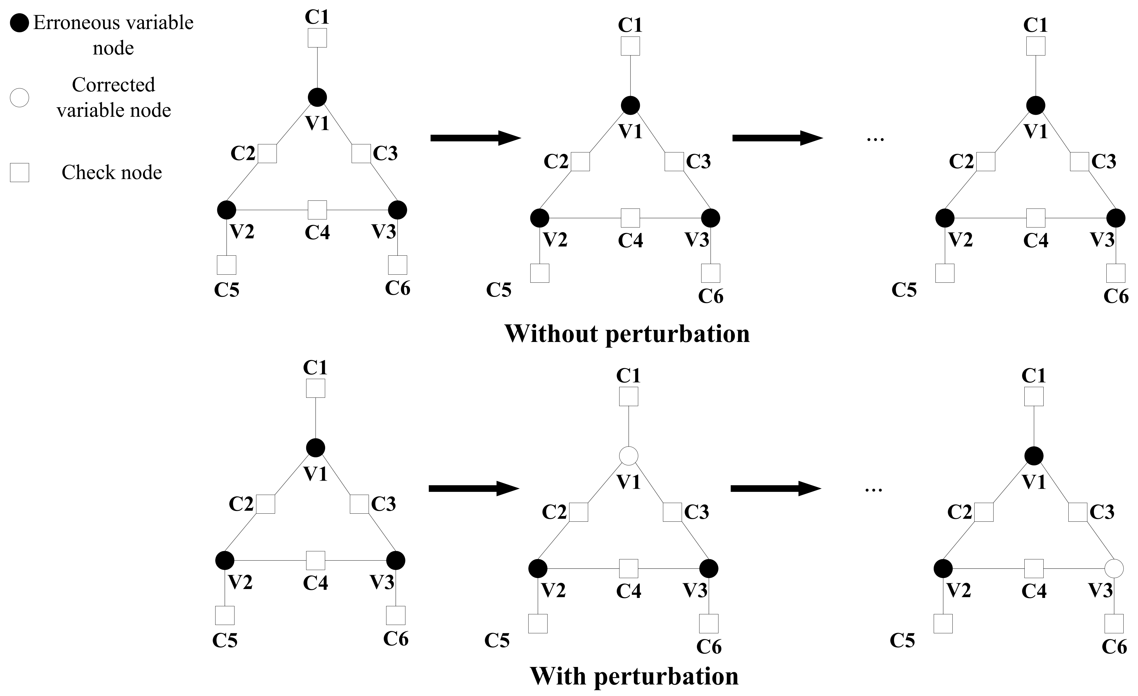
Figure 6 shows a (6, 3) trapping set of three variable nodes that remain erroneous during iterations and may be corrected with perturbation in check-to-variable messages. Since all three variable nodes are incorrect, perturbation here may flip their signs and therefore will not hinder BP decoding but rather provide the possibility for error correction. However, a simple (6, 3) trapping set here contains 9 nodes and 9 edges, and it is impossible to use the whole Tanner graph of the LDPC code to analyze the gain of perturbation and yield a closed-form expression. We used Monte Carlo simulations to evaluate its performance.

3.4. RS Parallel Encoder

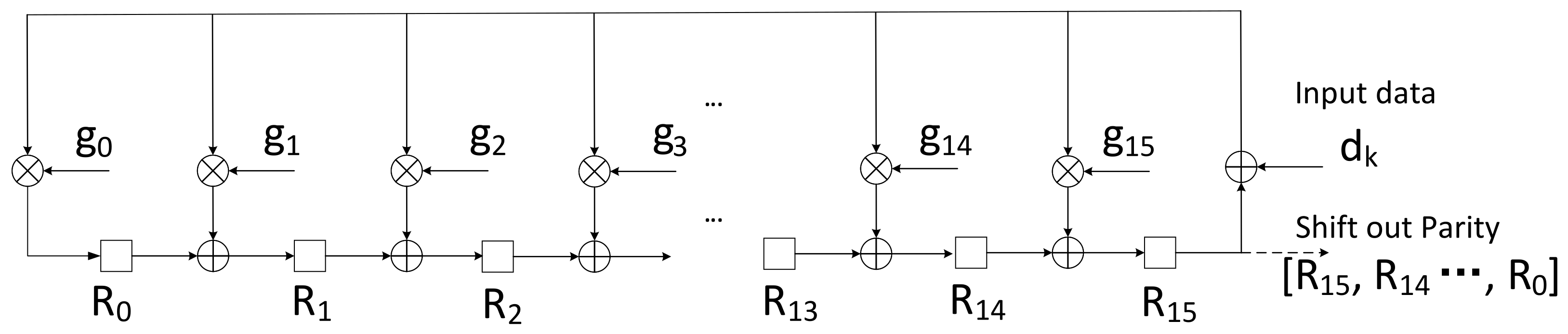
The conventional RS encoder adopts a serial structure that can be treated as a digital circuit. It consists of shifting registers and constant multipliers [26], depicted in Figure 7, whose control, initialization, and reset logic are not depicted here. There are 20 shifting registers and 20 constant multipliers for RS (340, 320) code together with 20 adders (bitwise XOR). After data $d_k$ are serially input, contents of registers are serially shifted out in the sequence of $R_{19},R_{18},\dots ,R_0$, which are parity bits, accordingly.

For RS (340, 320) code, let the input data be $\mathit{d}=\left\{d_k\right\}$, where $k=0,1,\dots ,319$ is the index of the clock period in this digital circuit of the encoder, and the generator polynomial is $g\left(x\right)=x^{20}+g_{19}{x}^{19}+\dots +g_{1}x+g_0$, whose coefficients $[g_{19},\dots ,g_0]=$ [58, 257, 157, 222, 388, 151, 62, 280, 137, 404, 286, 394, 61, 399, 73, 84, 145, 293, 369, 331] are constant. Shifting register $R_n\left(k\right)$ describes the value of register n at clock period k, where $n=0,1,\dots ,19$. We formulated the serial encoder as

$$R_n(k+1)=\left\{\begin{array}{cc}{R}_{n-1}\left(k\right)+\hfill & (d_k+R_{19}\left(k\right))g_n,n\ge 1,\hfill \\ \hfill & (d_k+R_{19}\left(k\right))g_n,n=0.\hfill \end{array}\right.$$

(22)

Furthermore, initial states $R_n\left(0\right)=0$ for all registers. After 320 clock periods, all data are input into the encoder, all adders and multipliers are stopped, and 20 registers are shifted out in the sequence of $[R_{19}\left(320\right),R_{18}\left(320\right),\dots ,R_0\left(320\right)]$ to constitute the parity part of the RS (340, 320) code. In fact, the calculation performed by this encoder is equivalent to $x^{20}+R_{19}{x}^{19}+\dots +R_{1}x+R_0=(((d_{0}g\left(x\right)\times x+d_{1}g\left(x\right))\times x+\dots +d_{318}g\left(x\right))\times x+d_{319}g\left(x\right)modg\left(x\right)$.

$$\begin{array}{cc}\hfill R_5(k+4)& =R_4(k+3)+(d_{k+3}+R_{19}(k+3))g_5\hfill \\ \hfill & =\dots \hfill \\ \hfill & =R_1\left(k\right)+(d_{k+3}+R_{16}\left(k\right))g_5+(d_{k+2}+R_{17}\left(k\right))(g_4+g_{19}{g}_5)+(d_{k+1}+R_{18}\left(k\right))(g_3+g_{19}{g}_4+(g_{18}+g_{19}^2)g_5)\hfill \\ \hfill & +(d_k+R_{19}\left(k\right))(g_2+g_{19}{g}_3+(g_{18}+g_{19}^2)g_4+(g_{17}+2g_{18}{g}_{19}+g_{19}^3)g_5).\hfill \end{array}$$

(23)

$$\begin{array}{cc}{R}_n(k+4)=\hfill & \hfill \end{array}$$

$$\hspace{1em}\hspace{1em}\left\{\begin{array}{cc}{R}_{n-4}\left(k\right)+\hfill & (d_k+R_{19}\left(k\right))p_n\left(0\right)+(d_{k+1}+R_{18}\left(k\right))p_n\left(1\right)+(d_{k+2}+R_{17}\left(k\right))p_n\left(2\right)+(d_{k+3}+R_{16}\left(k\right))p_n\left(3\right),n\ge 4,\hfill \\ \hfill & (d_k+R_{19}\left(k\right))p_n\left(0\right)+(d_{k+1}+R_{18}\left(k\right))p_n\left(1\right)+(d_{k+2}+R_{17}\left(k\right))p_n\left(2\right)+(d_{k+3}+R_{16}\left(k\right))p_n\left(3\right),n=0,1,2,3.\hfill \end{array}\right.$$

(24)

The shortcomings of a serial encoder are low throughput and high encoding latency. We accordingly require a new structure to encode in parallel and lower the encoding latency while improving its throughput. Considering a 4-parallel encoder, each clock period during operation should be equivalent to four clock periods in the serial encoder. By carefully observing (22) and Figure 7, we can see that $R_n(k+1)$ is determined by two variable terms $R_{n-1}\left(k\right)$ (except for $R_0$) and $(d_k+R_{19}\left(k\right))$. By recursively applying (22), $R_n(k+4)$ is determined by five variable terms: $R_{n-4}\left(k\right)$ (except for $R_0,R_1,R_2,R_3$), $(d_k+R_{19}\left(k\right))$, $(d_{k+1}+R_{18}\left(k\right))$, $(d_{k+2}+R_{17}\left(k\right))$, and $(d_{k+3}+R_{16}\left(k\right))$. We take $R_5(k+4)$ for example, as in (23), which is clearly especially complicated to derive and difficult to understand. In order to simplify the derivation, we came up with an easy approach for calculating parallel encoding coefficients, leveraging a conventional serial encoder structure.

We came up with a method to use the serial encoder to calculate the parallel encoding coefficients and propose it as Algorithm 2. The details of its derivation are described in the Appendix A.

Algorithm 2 Parallel Encoding Coefficient Calculation.

Initialize the serial encoder; set all registers to zero.      Input: “1”. Run one clock and $p_n\left(3\right)\leftarrow R_n\left(1\right)$.      Input: “0”. Run one clock and $p_n\left(2\right)\leftarrow R_n\left(2\right)$.      Input: “0”. Run one clock and $p_n\left(1\right)\leftarrow R_n\left(3\right)$.      Input: “0”. Run one clock and $p_n\left(0\right)\leftarrow R_n\left(4\right)$. Return: $p_n\left(3\right),p_n\left(2\right),p_n\left(1\right),p_n\left(0\right)$.

An example of a 4-parallel encoder structure is given in Figure 8. Other parallelism implementations are very similar to the 4-parallel scenario.

4. Performance Evaluation, Results, and Discussion

We carried out simulations to evaluate the proposed concatenation code and decoding algorithm. The simulations were performed with FTN signaling, $\tau =0.703$, and shortened $\mathit{v}=[0.553,0.793,-0.084,-0.171,0.154,-0.064]$. We used $\mathit{y}=\mathit{a}\ast \mathit{v}$ as in (4) to model the received signal through the AWGN channel, detect it with the 4-BCJR method, and then decode the channel code and perform turbo equalization. Finally, we computed the BER to evaluate each decoding scheme at different SNRs. To reduce storage used for the BCJR trellis, we limited states at each stage to M = 4. Moreover, we set the number of turbo equalization iterations to 3 to avoid excessive iterations for the LDPC decoder and decrease the decoding time. The LDPC code used here is a (7680, 3840) code defined by the 5G standard mentioned in Section 2, with 780 data bits shortened (around 10%) to the lower code rate, leading to more definite results. RS (340, 320) is a 0.94 high-rate code with 6% parity redundancy. The shortening of the LDPC and simple hard decision RS concatenation scheme shows the ability to lower the error floor of original LDPC-coded FTN signaling and has an overall code rate of 0.42. All simulations were performed with MATLAB 2022 on a CPU; no GPU was used.

Note that the demonstration of the proposed scheme is intended to show its effectiveness in lowering the error floor, and parameters of shortening and RS code can change with different code rates vs. the BER and with different LDPC code. Thus, those parameters can be determined by practical means and trade-offs and are not required to be optimal since the goal of the proposed scheme is to lower the error floor.

The BP decoders with maximum iteration limits of 20 and 50 also show an error floor of around ${10}^{-5}$. The concatenation code lowers the error floor to $4\times {10}^{-6}$, and no error floor was found in the simulations of the concatenation code with perturbation in the BP decoder down to $2\times {10}^{-7}$ and $4\times {10}^{-8}$, as depicted in Figure 9 and Figure 10, respectively. We found that, for three iterations of turbo equalization, increasing the iteration number of the LDPC code has little effect on the BER performance.

The saturation (no more decrease) of the red curve and the blue curve in Figure 9 and the green curve and the red curve in Figure 10 are caused by residual relevance (interference) between symbols. From the view of the decoder, residual relevance leads to error propagation especially with trapping sets in the factor graph. We utilize high-rate RS code to lower the error floor, but it still exists, which means concatenating RS code is helpful, but high-rate RS is inadequate for eliminating the error floor. We introduce perturbation decoding to enhance the proposed LDPC-RS concatenation scheme and eliminate the error floor.

In [6], LDPC-RS product code and the hybrid error–erasure correction (HEEC) decoding algorithm were proposed. The difference is that our proposed approach utilizes concatenated code, i.e., a whole RS code word is treated as the information part of an LDPC code word. Additionally, [6] utilizes product code, in which multiple RS code words are put in columns and multiple LDPC codes are put in rows. LDPC (576, 288)-RS (255, 51) product code (code length 576 × 255) and HEEC decoding in [6] will have better performance than our proposed scheme. However, since product code is deeply coupled, RS decoding can only start after 255 LDPC codes finish decoding. The product code consists of 255 LDPC codes and 36 RS codes. The overall decoding latency is $(255\times Latency(LDPC)+36\times Latency(RS\left)\right)\times Iteration$, where $Latency\left(LDPC\right)$ and $Latency\left(RS\right)$ may vary from different decoding algorithms. For the LDPC-RS concatenation scheme proposed in this paper, the overall decoding latency is $\left(Latency\right(LDPC)+Latency(RS\left)\right)\times Iteration$. The storage required by product code in [6] is $255\times Storage\left(LDPC\right)+36\times Storage\left(RS\right)$, while our proposed scheme needs $Storage\left(LDPC\right)+Storage\left(RS\right)$. Therefore, product code in [6] introduces much more latency and needs much more storage than our proposed concatenated code. For our proposed scheme, RS decoding only needs to wait for one LDPC code to finish decoding. Additionally, the HEEC iterative decoding exchanges information between the LDPC and RS decoders. Therefore, decoding latency increases in proportion to iterations. Our proposed scheme does not use iterative decoding between LDPC and RS code considering the increase in latency. In [11], Qiu and coworkers achieved a similar level (${10}^{-8}$ to ${10}^{-7}$) of noise floor with their RS-SC-LDPC algorithm. Spatially coupled LDPC code may have better performance; however, it has much more complexity and latency, even when utilizing sliding window decoding. Meanwhile, SC or sliding window decoding needs more storage for multiple LDPC code words. Product code scheme or spatially coupled code scheme will have better performance than our proposed concatenated code scheme. However, while considering constraints on latency, complexity, and storage, our proposed scheme will be a better choice.

5. Conclusions

In this paper, we demonstrate 5G LDPC (7680, 3840) code in FTN signaling to explore spectrum efficiency and reliability. When limited to low latency and low storage, i.e., few BCJR states and few turbo iterations, we found an undesirable error floor. To combat the error floor, we proposed one possible solution, namely, using the LDPC-RS concatenation and shortening scheme together with perturbation introduced into the BP decoder, where the LDPC has a rate of 0.5 as well as a 0.94 high-rate hard decision RS code to lower the rate loss. We proposed a 4-parallel encoder architecture for RS component code and a concise algorithm to calculate its constant multiplier coefficients, leveraging a traditional serial encoder. This algorithm can also be used for calculating other parallelisms, code rates, and lengths. The simulation results show that the proposed concatenation and shortening scheme can lower the error floor of the original single LDPC code, and with perturbation in the BP decoder, the error floor can be eliminated below ${10}^{-7}$ for different LDPC maximum decoding iterations. The advantage of the proposed scheme is that the LDPC has an error correction ability for BCJR detection with few states and few iterations of turbo equalization FTN signaling, while RS concatenation, shortening, and perturbation techniques together lower the error floor. In future research, other LDPC codes will be constructed, factor graph-based FTN detection with LDPC joint decoding will be explored, and LDPC-RS soft iteration decoding will also be studied. A better equalizer will also be studied to strengthen and broaden the LDPC-RS concatenation scheme’s implementation for fading channels and other scenarios.

References

- Anderson, J.B.; Rusek, F.; Öwall, V. Faster-Than-Nyquist Signaling. Proc. IEEE 2013, 101, 1817–1830. [Google Scholar] [CrossRef]
- Prlja, A.; Anderson, J.B. Reduced-Complexity Receivers for Strongly Narrowband Intersymbol Interference Introduced by Faster-than-Nyquist Signaling. IEEE Trans. Commun. 2012, 60, 2591–2601. [Google Scholar] [CrossRef]
- Che, D.; Chen, X. Higher-Order Modulation vs Faster-Than-Nyquist PAM-4 for Datacenter IM-DD Optics: An AIR Comparison Under Practical Bandwidth Limits. J. Light. Technol. 2022, 40, 3347–3357. [Google Scholar] [CrossRef]
- Gallager, R. Low-density parity-check codes. IRE Trans. Inf. Theory 1962, 8, 21–28. [Google Scholar] [CrossRef]
- Chung, S.Y.; Forney, G.; Richardson, T.; Urbanke, R. On the design of low-density parity-check codes within 0.0045 dB of the Shannon limit. IEEE Commun. Lett. 2001, 5, 58–60. [Google Scholar] [CrossRef]
- Chen, W.; Wang, T.; Han, C.; Yang, J. Erasure-correction-enhanced iterative decoding for LDPC-RS product codes. China Commun. 2021, 18, 49–60. [Google Scholar] [CrossRef]
- Chen, W.; Yin, L.; Lu, J. Minimum distance lower bounds for girth-constrained RA code ensembles. IEEE Trans. Commun. 2010, 58, 1623–1626. [Google Scholar] [CrossRef]
- Zhang, Z.; Dolecek, L.; Nikolic, B.; Anantharam, V.; Wainwright, M. Design of LDPC decoders for improved low error rate performance: Quantization and algorithm choices. IEEE Trans. Commun. 2009, 57, 3258–3268. [Google Scholar] [CrossRef]
- Kyung, G.B. Finding the Exhaustive List of Small Fully Absorbing Sets and Designing the Corresponding Low Error-Floor Decoder. IEEE Trans. Commun. 2012, 60, 1487–1498. [Google Scholar] [CrossRef]
- Dolecek, L.; Lee, P.; Zhang, Z.; Anantharam, V.; Nikolic, B.; Wainwright, M. Predicting error floors of structured LDPC codes: Deterministic bounds and estimates. IEEE J. Sel. Areas Commun. 2009, 27, 908–917. [Google Scholar]
- Qiu, J.; Chen, L.; Liu, S. A Novel Concatenated Coding Scheme: RS-SC-LDPC Codes. IEEE Commun. Lett. 2020, 24, 2092–2095. [Google Scholar] [CrossRef]
- Urard, P.; Paumier, L.; Georgelin, P.; Michel, T.; Lebars, V.; Yeo, E.; Gupta, B. A 135Mbps DVB-S2 compliant codec based on 64800-bit LDPC and BCH codes (ISSCC Paper 24.3). In Proceedings of the 42nd Design Automation Conference, Anaheim, CA, USA, 13–17 June 2005; pp. 547–548. [Google Scholar]
- Rasheed, O.A.; Ivanis, P.; Vasic, B. Fault-Tolerant Probabilistic Gradient-Descent Bit Flipping Decoder. IEEE Commun. Lett. 2014, 18, 1487–1490. [Google Scholar] [CrossRef]
- Vasić, B.; Ivanis, P.; Brkic, S.; Ravanmehr, V. Fault-resilient decoders and memories made of unreliable components. In Proceedings of the 2015 Information Theory and Applications Workshop (ITA), San Diego, CA, USA, 1–6 February 2015; pp. 136–142. [Google Scholar]
- Ivanis, P.; Al Rasheed, O.; Vasić, B. MUDRI: A fault-tolerant decoding algorithm. In Proceedings of the 2015 IEEE International Conference on Communications (ICC), London, UK, 8–12 June 2015; pp. 4291–4296. [Google Scholar]
- Ivaniš, P.; Vasić, B.; Declercq, D. Performance evaluation of faulty iterative decoders using absorbing Markov chains. In Proceedings of the 2016 IEEE International Symposium on Information Theory (ISIT), Barcelona, Spain, 10–15 July 2016; pp. 1566–1570. [Google Scholar]
- Ivanis, P.; Brkic, S.; Vasić, B. Stochastic resonance in iterative decoding: Message passing and gradient descent bit flipping. In Proceedings of the 2017 13th International Conference on Advanced Technologies, Systems and Services in Telecommunications (TELSIKS), Nis, Serbia, 18–20 October 2017; pp. 300–307. [Google Scholar]
- Reed, I.S.; Solomon, G. Polynomial Codes Over Certain Finite Fields. J. Soc. Ind. Appl. Math. 1960, 8, 300–304. [Google Scholar] [CrossRef]
- Mazo, J.E. Faster-Than-Nyquist Signaling. Bell Syst. Tech. J. 1975, 54, 1451–1462. [Google Scholar] [CrossRef]
- Wu, R.; Wang, L.; Yuan, T.; Wang, M. Improved MS LDPC Decoder Based on Jacobian Logarithm. In Proceedings of the 2019 7th International Conference on Information, Communication and Networks (ICICN), Macao, China, 24–26 April 2019; pp. 53–56. [Google Scholar]
- Chen, J.; Fossorier, M.P.C. Near optimum universal belief propagation based decoding of low-density parity check codes. Commun. IEEE Trans. 2002, 50, 406–414. [Google Scholar] [CrossRef]
- Ding, J.; Shi, H.; Luo, Z. Joint SB/NMS and Genetic Optimization for High Performance LDPC Decoding. In Proceedings of the 2022 International Symposium on Networks, Computers and Communications (ISNCC), Shenzhen, China, 19–22 July 2022; pp. 1–6. [Google Scholar]
- Shi, H.; Zhong, M.; Luo, Z.; Li, C. Low Complexity Neural Network-Aided NMS LDPC Decoder. In Proceedings of the 2021 Computing, Communications and IoT Applications (ComComAp), Shenzhen, China, 24–26 April 2019; pp. 227–231. [Google Scholar]
- Richardson, T.; Kudekar, S. Design of Low-Density Parity Check Codes for 5G New Radio. IEEE Commun. Mag. 2018, 56, 28–34. [Google Scholar] [CrossRef]
- Ivaniš, P.; Vasić, B. Error Errore Eicitur: A Stochastic Resonance Paradigm for Reliable Storage of Information on Unreliable Media. IEEE Trans. Commun. 2016, 64, 3596–3608. [Google Scholar] [CrossRef]
- Tang, Y.J.; Zhang, X. Low-Complexity Resource-Shareable Parallel Generalized Integrated Interleaved Encoder. IEEE Trans. Circuits Syst. I Regul. Pap. 2022, 69, 694–706. [Google Scholar] [CrossRef]