
An Algorithm for Distracted Driving Recognition Based on Pose Features and an Improved KNN

School of Electrical and Electronic Engineering, Shanghai Institute of Technology, Shanghai 201418, China
*
Author to whom correspondence should be addressed.
Electronics 2024, 13(9), 1622; https://doi.org/10.3390/electronics13091622
Submission received: 1 April 2024
/
Revised: 18 April 2024
/
Accepted: 19 April 2024
/
Published: 24 April 2024
Abstract
:To reduce safety accidents caused by distracted driving and address issues such as low recognition accuracy and deployment difficulties in current algorithms for distracted behavior detection, this paper proposes an algorithm that utilizes an improved KNN for classifying driver posture features to predict distracted driving behavior. Firstly, the number of channels in the Lightweight OpenPose network is pruned to predict and output the coordinates of key points in the upper body of the driver. Secondly, based on the principles of ergonomics, driving behavior features are modeled, and a set of five-dimensional feature values are obtained through geometric calculations. Finally, considering the relationship between the distance between samples and the number of samples, this paper proposes an adjustable distance-weighted KNN algorithm (ADW-KNN), which is used for classification and prediction. The experimental results show that the proposed algorithm achieved a recognition rate of 94.04% for distracted driving behavior on the public dataset SFD3, with a speed of up to 50FPS, superior to mainstream deep learning algorithms in terms of accuracy and speed. The superiority of ADW-KNN was further verified through experiments on other public datasets.
1. Introduction
According to data released by the World Health Organization, car accidents are the leading cause of death after diseases and wars. Globally, approximately 1.35 million people die in car accidents each year, and tens of millions more are disabled [1]. Road traffic accidents are typically caused by subjective and objective factors. Subjective factors refer to the driver’s driving behavior, while objective factors often involve uncontrollable and unpredictable elements such as the environment and road conditions [2]. Many studies on the causes of car accidents [3,4,5] have identified distracted driving as a significant factor. Paper [3] indicates that approximately 45% of car accidents are directly caused by drivers’ lack of attention or drivers engaging in non-driving activities. Paper [6] mentions that using a mobile phone or answering calls while driving can slow down the driver’s reaction time, increasing the risk of accidents by four times. Paper [7], analyzing a large amount of accident data, suggests that young males are more prone to traffic accidents, possibly due to their tendency to engage in distracted behaviors such as chatting, smoking, and driving under the influence of alcohol. Until vehicles are fully autonomous, drivers will remain the direct decision-makers in the transportation system. Therefore, the accurate and rapid recognition of distracted driving behaviors is a crucial research direction for intelligent and safe driving [8].
Methods for detecting distracted driving can be broadly classified into three categories: based on driver physiological parameters, based on driving environment characteristics, and based on deep learning. Early scholars primarily used sensors to collect physiological signals from drivers to analyze distracted driving behaviors. For instance, Lin et al. conducted extensive research on the relationship between electroencephalography (EEG) and distracted driving [9,10,11] and found that when drivers are distracted, the power of theta and beta waves in the frontal region of the brain increases, with the magnitude reflecting the degree of distraction. Deshmukh et al. [12] greatly improved the ability to discriminate distracted driving by applying wavelet packet transform to electrocardiogram (ECG) signals.
Monitoring vehicle driving environment parameters is an indirect but accurate detection method. Kountouriotis et al. [13] conducted experiments on a driving simulator and concluded that visual distraction can increase the lateral deviation of the vehicle, especially during turns. Li et al. [14] collected and compared operational parameters such as steering wheel, throttle, and brake control under distracted and normal driving conditions, as well as vehicle driving parameters. Their results showed that drivers frequently compensate for driving parameters when distracted, leading to instability in the vehicle’s driving state.
In recent years, deep learning has achieved significant success in areas such as image classification and object recognition. Many scholars have attempted to use deep learning models to detect distracted driving behaviors [15], including ResNet and VGG [16,17]. Zhang et al. [18] compared the performance of ResNet-50 and VGG-16 in distracted driving recognition and ultimately constructed a detection model using an improved VGG-16. Ruthuparna et al. [19] developed a CNN model with only 9.5 MB of parameters that could effectively recognize distracted driving behaviors involving hand movements. Luo et al. [20] introduced a lightweight backbone network, GhostNet and GSConv, and YOLOv5 to reduce network parameters and achieve faster and more accurate recognition of common distracted behaviors such as answering phone calls, smoking, and drinking water. Li et al. [21] combined visual transformers (VITs) and convolutional neural networks (CNNs) to more fully capture local and global image features. Wei et al. [22] constructed a graph convolutional network using a driver’s skeletal model and fused key target information, achieving an accuracy of 86% on a self-constructed distracted driving dataset.
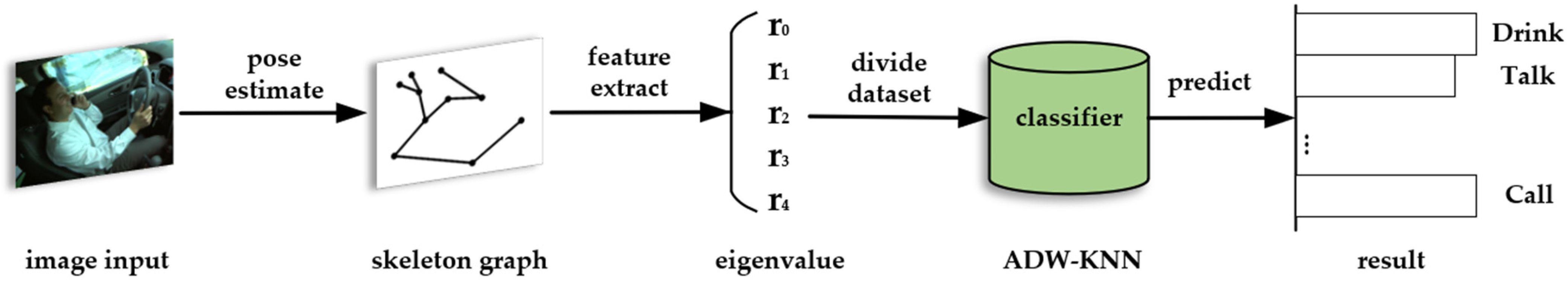
Overall, sensor-based methods are direct and effective but limited by their high hardware costs and inconvenience for passengers and drivers. Deep learning models offer high accuracy and recognition speeds but pose challenges for hardware deployment due to their large model parameters. Therefore, this paper proposes an algorithm that utilizes deep learning to extract driver posture features and combines them with an improved KNN for classification, as shown in Figure 1. This approach combines the feature extraction capabilities of deep learning models with the rapid classification and recognition abilities of machine learning. Our work is roughly as follows:
- (1)
- Extract key points of a driver’s body using a lightweight pose detection framework to construct a sequence diagram of the driver’s behavioral skeleton.
- (2)
- Establish a mathematical model of driving behavior based on ergonomic principles and calculate feature quantities.
- (3)
- Input the obtained feature data into an improved KNN model and, finally, output the recognition result.
- (4)
- Validate the proposed algorithm through comparison experiments with other algorithms, demonstrating its advantages of fast execution speed and high accuracy.
2. Pose Estimation
Human pose estimation can be described as a method that reconstructs the human skeleton by extracting information on the locations of key points on the human body and estimating the relationships between these key points. Pose estimation has important applications in areas such as action recognition, action tracking, human–computer interaction, and so on. Among them, typical pose estimation algorithms include DeepPose [23], CMPs (convolutional pose machines) [24], OpenPose [25], and others.
2.1. Lightweight OpenPose
Lightweight OpenPose [26] is a classic, lightweight version of OpenPose that significantly improves the model’s running speed at the cost of almost negligible accuracy loss. The general process is outlined as follows: Firstly, an image is fed into the feature extraction network, MobileNet, to extract shallow semantic information and obtain feature map F. This feature map then enters the first stage, where it undergoes a series of CNN operations, ultimately outputting two branches. The first branch, , is responsible for generating part confidence maps (PCMs) around the joint points in the image, indicating the level of confidence. The second branch, , predicts part affinity fields (PAFs), which represent the position and possible connection directions of the joint points in vector form.
From the second stage onward, the network’s input integrates three components from the previous stage: , , and , as shown in Equation (1). Within the second stage, the consolidated input features undergo numerous convolutions with kernel sizes of 1 × 1 and 3 × 3, connected by skip structures. This process iterates through n − 1 such CNN structures. The losses of each branch are calculated using the L2 loss function, and the positions of each joint are output once the losses converge. The Hungarian matching algorithm is then employed to find the best adjacent joint points and, finally, all suitable joint points are connected in order to output the human skeleton structure. The general process is schematically illustrated in Figure 2.
2.2. Skeleton Pruning
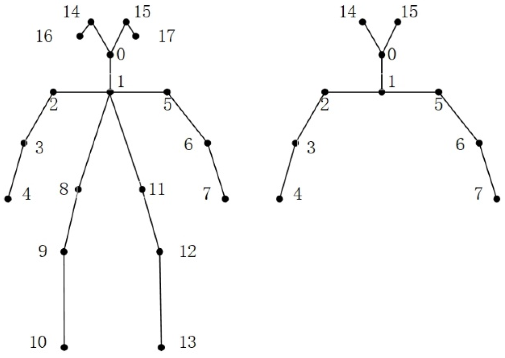
The original pose estimation framework was trained based on the COCO dataset, which detected 18 key points on the human body, following the COCO annotation format (as shown in Figure 3, left). However, the target of detection was a driver inside a vehicle, and driving behaviors are generally expressed through upper body movements. Due to the driving environment, the lower body parts of the driver may be inevitably occluded, and certain body parts may be difficult to detect effectively due to individual differences among drivers. Therefore, to eliminate these effects, this study did not identify key points that could cause interference or that did not contribute to the judgment of distracted driving behaviors. It discarded all lower body parts (8–13) as well as the left ear (16) and right ear (17). Instead, pose estimation was only performed on 10 key points of the upper body (as shown in Figure 3, right), specifically the following 10 key points: (0) nose, (1) neck, (2) right shoulder, (3) right elbow, (4) right wrist, (5) left shoulder, (6) left elbow, (7) left wrist, (14) right eye, and (15) left eye.
By reducing the original 19 heatmaps, including the background, to 11 and then feeding them into the branches for training, several benefits were achieved: (1) The number of key points calculated by the PCMs was reduced from 18 to 10, meaning that the number of channels in branch 1 became 10. (2) The number of output channels in PAFs equaled the number of bone segments multiplied by 2, which represented the number of bones times two. Therefore, the number of channels in branch 2 was reduced to 22, significantly fewer than the original 38. This reduction in the number of parameters during multi-stage CNN operations accelerated the detection speed.
3. Feature Extraction
According to the principles of anthropometry, utilizing the angles and distances between key points can result in a better representation of a driver’s driving state [27]. Taking the skeleton sequence diagram of a single driver’s normal driving state as an example, as shown in Figure 4, the coordinates of key point i were denoted as and the Euclidean distance between two key points could be expressed as
The angle between two segments of bones could be calculated using the cosine theorem:
Most of the research on distracted driving includes behaviors such as using a mobile phone, eating, making phone calls, etc. [28,29]. These behaviors are typically expressed through the upper body. By calculating and abstracting the driver’s skeletal sequence diagram into a set of five-dimensional feature values , combined features could effectively describe abnormal behaviors in various body parts. The calculation methods for each feature value are given by Equations (4)–(8).
By defining placing both hands on the steering wheel, maintaining an upright posture, and keeping the head facing forward as the standard for normal driving status, the five-dimensional characteristic values of normal driving were set as standard quantities ▲▲. When there were one or three triangles, the corresponding feature values were smaller or larger than under normal driving conditions. The characteristic patterns under different driving behaviors were established as shown in Table 1.
4. Classification Algorithms
While currently mainstream deep learning algorithms exhibit excellent performance in classification tasks, most of them achieve feature extraction through the deep stacking of convolutional neural networks and then output class confidence through a classification function [30,31,32]. However, these extensive computations place higher demands on the computational power of devices. Traditional machine learning theory has been highly developed over a long period of time, possessing strong interpretability and practical application value. Based on sufficient feature engineering, classification results can be obtained through rapid numerical calculations.
4.1. KNN
KNN is a classical machine learning method that is widely used for solving classification and regression problems due to its simple principle and excellent performance. Its main idea is to iterate through the K nearest values in the training set and conduct voting, with the predicted result being the category that receives the majority of votes, as shown in Figure 5.
In the KNN algorithm, commonly used distance metrics mainly include Euclidean distance and Manhattan distance. The mathematical expressions for these metrics are given by Equations (9) and (10), respectively, where V represents the number of feature value dimensions.
The value of K in the KNN algorithm is a parameter that requires repeated validation as its selection greatly affects the performance on the test set. When the chosen K value is too small, the voting objects are limited to a very small region, and the prediction result depends heavily on the most similar values between the training set and the test set, which can be easily influenced by outliers. Conversely, when the chosen K value is too large, the range of voting objects increases, which not only increases the computational burden of the algorithm but also raises the risk of overfitting. Therefore, it is crucial to select an appropriate K value based on the characteristics of the dataset for accurate predictions. Generally, we need to start with a small odd value of K (usually K = 1) and gradually increase it for experiments to select the appropriate K value.
4.2. ADW-KNN
However, the traditional KNN algorithm simply considers the importance of the majority proportion among voters, while ignoring the specific positional relationships among them. This can lead to issues such as the following: As shown in Figure 5, if only the majority proportion of votes is considered to determine the predicted value, then the predicted result would be a triangle. In reality, considering the positions of the voters and the predicted value, the predicted result often tends to be a circle. Furthermore, in traditional KNN, K is generally only taken as an odd number. The reason for this is that when K is an even number, there is a high possibility of a draw situation where the number of votes for each category is the same, as illustrated in Figure 6.
To address the aforementioned issues, this paper proposes an adjustable parameter KNN classification method (ADW-KNN) that incorporates distance as a basis for voting. The main idea is to no longer rely solely on majority voting to determine the predicted result but instead to combine category counts and distances as indicators for prediction. By introducing an adjustable parameter P, different weights can be assigned to these two indicators to finalize the output. The benefit of this approach is that it introduces positional references among voters, which helps to mitigate the influence of outliers when the value of K is small and enables more accurate identification of training data with the highest similarity to the predicted value. Additionally, it effectively resolves ties when K is an even number.
The main calculation process (Figure 7) of ADW-KNN involved selecting the K nearest voters, calculating the category contribution ratio and distance contribution ratio for each category among the voters. The category contribution ratio was defined as the ratio of the total number of votes for each category to the total number of voters (K). The distance contribution ratio was defined as the ratio of the reciprocal sum of distances for each category to the reciprocal sum of distances for all voters. Finally, the overall weight w was calculated, and the category with the highest weight was output as the predicted result.
The formula representation of the main parameters involved in the above process is as follows:
The distance calculation involved in ADW-KNN is obtained based on Euclidean distance (such as Formula (9)). P is an adjustable parameter between 0 and 1, it is used to adjust the weights of category contribution and distance contribution. When P = 1, it corresponds to the traditional KNN algorithm.
5. Experimental Preparation
5.1. Introduction to the Dataset
Currently, there are relatively few publicly available distracted driving behavior datasets, and their quality varies greatly. Therefore, the experimental data used in this article were derived from the large-scale dataset State Farm Distracted Driver Detection (SFD3) [33], which is publicly available on the well-known machine learning competition website Kaggle. Eight types of high-risk distracted behaviors were selected for the experiment, totaling over 18,000 images with a uniform size of 640 × 480 RGB. Part of the dataset is shown in Figure 8, and the processed dataset is shown in Figure 9. All images were randomly divided into training and testing sets in an 8:2 ratio, as shown in Table 2. The following table shows the number of images in the training and testing sets for each category.
5.2. Experimental Environment
The experiment was conducted on a desktop computer running Windows 10. The model code was developed using the Python–PyTorch software package (Python version 3.9.13 and PyTorch version 1.8.1). Some parts of the code were written in the Cython language, with Cython version 3.0.0. The computer had the following specifications: CPU Model: Core i5-7300HQ; RAM: 8 GB; GPU Model: GTX 1050ti; VRAM: 4 GB.
5.3. Evaluation Index
Accuracy is generally used as an evaluation indicator for the predictive ability of a model. The calculation formula is below:
TP represents positive samples predicted as positive, TN represents negative samples predicted as negative, FP represents negative samples predicted as positive, and FN represents positive samples predicted as negative.
To measure the detection speed of a model, FPS is generally used as an evaluation metric, defined as the number of images detected by the model per second, measured in Hz.
6. Experimental and Results Analysis
6.1. Comparison Experiment between KNN and ADW-KNN
The goal was to validate the superiority of ADW-KNN compared to the traditional KNN algorithm. The feature vectors obtained were classified using both the KNN and ADW-KNN algorithms. The specific experimental parameters were as follows: K ranges from 1 to 8 with a step size of 1. Adjustable parameter P ranges from 0.2 to 0.8 with a step size of 0.2.
Figure 10 compares the accuracy of the two algorithms. It can be observed that the KNN algorithm achieved the optimal classification result when K = 1 and 3, with an accuracy of 93.62%. However, the accuracy gradually decreased as K increased beyond 3, reaching a minimum of 92.26%. By adjusting the values of P and K to find the optimal parameters, Figure 10 shows that the highest prediction accuracy of 94.04% was achieved when K = 6 and P = 0.2. This was an improvement of 0.42% compared to the best accuracy of the KNN algorithm and a 1.28% increase compared to the accuracy when K = 6. As P increased with a step size of 0.2, it was found that the accuracy remained unchanged for K = 1 and 2 regardless of the value of P. For other values of K, the curve exhibited a general downward trend, with a more significant decrease as P approached 1. The experiments demonstrated that the ADW-KNN algorithm outperformed the KNN algorithm for the given range of P values, indicating that the improved algorithm achieves better classification results.
To further investigate the classification performance of both the KNN and ADW-KNN algorithms for various distracted driving behaviors, a comparison was made between their respective best and worst performances. The resulting confusion matrices are presented in Figure 11.
The analysis of the confusion matrices showed that the two algorithms had poor recognition rates for the three behaviors of (a) drinking, (d) texting right, and (f) calling right. The reason is that these three behaviors all occur in the right hand, resulting in small differences in characteristics between the behaviors and easy confusion among the three behaviors. Therefore, the recognition accuracy was lower than for other behaviors. Analyzing the confusion matrix in Figure 11, under the same K value, ADW-KNN showed a significant improvement in accuracy compared to KNN for both (d) texting right and (f) calling right. Overall, the accuracy of the improved algorithm was better than that of the original algorithm.
6.2. Comparison Experiment between ADW-KNN and Other Machine Learning Algorithms
To validate the superiority of the proposed ADW-KNN algorithm compared to other machine learning algorithms, classification experiments were conducted on the feature set obtained from the SFD3 dataset using algorithms such as decision tree (DT), support vector machine (SVM), and logistic regression (LR). Accuracy and computation time were compared across these algorithms. The best performance parameters for KNN and ADW-KNN were K = 1 and K = 6 with P = 0.2. For the decision tree algorithm, the entropy criterion was tested using Gini, cross-entropy, and log functions. SVM was evaluated using three kernel functions: rbf, linear, and sigmoid. For logistic regression, both L2 and L1 penalty functions were compared. The experimental results are presented in Figure 12, Table 3 shows the performance distribution of each algorithm under various conditions.
Based on the comprehensive analysis presented above, the ADW-KNN algorithm exhibits significant advantages in both accuracy and speed compared to other machine learning algorithms. Therefore, it was reasonable and effective to choose the KNN algorithm as the baseline for classification and further improvement. The ADW-KNN algorithm’s performance demonstrated its suitability for addressing the problem of distracted driving behavior recognition, offering a reliable and efficient solution.
6.3. The Generalization Experiment of ADW-KNN
To validate the generalization capability of the proposed ADW-KNN algorithm, we selected two representative, publicly available, machine learning datasets from the Kaggle website for performance testing.
- (1)
- Wine Quality Dataset [34]: This dataset consists of approximately 4900 wine samples, with 11 physicochemical properties as evaluation indicators. The quality of each wine is rated on a scale of 3–9, with a total of seven levels.
- (2)
- Wisconsin Breast Cancer Dataset [35]: This dataset comprises around 570 instances of patient information, with 30 clinical examinations and medical imaging data for each patient. The ultimate evaluation of a tumor is benign or malignant.
Both datasets were randomly divided into training and testing sets in an 8:2 ratio. KNN and ADW-KNN algorithms were employed for experimental analysis, and the results are presented in Figure 13. For ADW-KNN, the parameter P was set with a step size of 0.2.
From Figure 13a, it can be seen that when P = 0.2 and K = 8, ADW-KNN exhibited the highest accuracy of 64.3%, while KNN with the same K value only achieved an accuracy of 50.2%. When K was set to 1, KNN demonstrated its best accuracy of 60.7%. Overall, the improved KNN algorithm, ADW-KNN, performed relatively well on multi-class classification tasks.
Figure 13b illustrates that the performance of ADW-KNN remained consistent across various P values. It outperformed the KNN algorithm when K was set to 2 and 6. Both algorithms achieved the highest accuracy of 94.7%. In classification tasks with fewer categories, the ADW-KNN algorithm was not sensitive to changes in the P value. Adjusting the parameters did not lead to significantly better results than KNN, but it could outperform KNN in some cases when K was set to an even number.
6.4. Comparison Experiment between Our Algorithm and Other Algorithms
To validate the superiority of our algorithm, comparative experiments were conducted with some classic neural network models, such as VGG16, VGG19, and ResNet50, as well as algorithms proposed in recent years.
According to the experimental data in Table 4, compared with some classic CNN algorithms, the algorithm proposed in this paper has advantages in both accuracy and speed, especially in terms of accuracy, which is more powerful than that of CNNs.
Table 5 compares our algorithm with other algorithms. Paper [36] employed a MobileNet model based on transfer learning as the backbone for feature extraction, achieving approximately 90% accuracy while demonstrating a significant speed advantage with up to 100 FPS. The algorithm described in paper [37] innovatively utilizes ResNet50 for image feature extraction and then employs SVM for classification, resulting in the ReSVM algorithm achieving a high accuracy rate. However, the cascading of multiple models slows down the detection speed. In contrast, paper [38] lightweighted YOLOv8n and introduced an attention mechanism to create YOLOv8-LBS, demonstrating a good balance between accuracy and speed in experimental results.
7. Conclusions and Future Outlook
Currently, most algorithms for detecting driver distraction behaviors employ end-to-end deep learning models, while traditional machine learning algorithms struggle to handle such complex tasks. This paper innovatively proposes the use of deep learning as a means of feature extraction, combined with the rapid and accurate classification capabilities of machine learning for prediction output. This approach significantly addresses the cumbersome training and parameter-tuning processes of deep learning, as well as the requirement for high-performance hardware. The KNN algorithm has achieved good results in application, possibly due to the distinct features between different distracted driving behaviors, and has a strong ability to find similar features. Furthermore, the ADW-KNN algorithm proposed in this paper demonstrated excellent performance on a large dataset. However, a limitation is the need to adjust parameters through testing to find the appropriate values for P and K. Often, the K value for ADW-KNN is larger than that for the KNN algorithm, resulting in increased computational complexity.
Future work will focus on three main areas: (1) Constructing a dataset captured from the driver’s frontal view, enabling the pose estimation network to more easily extract driver pose features. (2) Embedding the algorithm into an in-vehicle image capture device to achieve end-to-end deployment and application. (3) Exploring the use of excellent ensemble learning algorithms, such as random forests, for feature classification, as experiments have shown that decision trees also exhibit promising classification performance and execution speed.
Author Contributions
Methodology, Y.G.; software, Y.G.; writing—original draft preparation, Y.G.; writing—review and editing, X.S. All authors have read and agreed to the published version of the manuscript.
Funding
This research received no external funding.
Data Availability Statement
The data presented in this study are available in the article.
Conflicts of Interest
The authors declare no conflicts of interest.
References
- Ahmed, S.K.; Mohammed, M.G.; Abdulqadir, S.O.; El-Kader, R.G.A.; El-Shall, N.A.; Chandran, D.; Rehman, M.E.U.; Dhama, K. Road traffic accidental injuries and deaths: A neglected global health issue. Health Sci. Rep. 2023, 6, e1240. [Google Scholar] [CrossRef] [PubMed]
- Pei, Y.; Ma, J. Research on countermeasures for road condition causes of traffic accidents. Chin. J. Highw. Transp. 2003, 16, 77–82. [Google Scholar]
- Touahmia, M. Identification of risk factors influencing road traffic accidents. Eng. Technol. Appl. Sci. 2018, 8, 2417–2421. [Google Scholar] [CrossRef]
- Stylianou, K.; Dimitriou, L.; Abdel-Aty, M. Big data and road safety: A comprehensive review. Mobil. Patterns Big Data Transp. Anal. 2019, 297–343. [Google Scholar]
- Bucsuházy, K.; Matuchová, E.; Zůvala, R.; Moravcová, P.; Kostíková, M.; Mikulec, R. Human factors contributing to the road traffic accident occurrence. Precedia Transp. Res. 2020, 45, 555–561. [Google Scholar] [CrossRef]
- Lipovac, K.; Đerić, M.; Tešić, M.; Andrić, Z.; Marić, B. Mobile phone use while driving-literary review. Transp. Res. Part F Traffic Psychol. Behav. 2017, 47, 132–142. [Google Scholar] [CrossRef]
- Hayashi, Y.; Foreman, A.M.; Friedel, J.E.; Wirth, O. Executive function and dangerous driving behaviors in young drivers. Transp. Res. Part F Traffic Psychol. Behav. 2018, 52, 51–61. [Google Scholar] [CrossRef] [PubMed]
- Nair, A.; Patil, V.; Nair, R.; Shetty, A.; Cherian, M. A review on recent driver safety systems and its emerging solutions. Int. J. Comput. Appl. 2024, 46, 137–151. [Google Scholar] [CrossRef]
- Lin, C.-T.; Lin, H.-Z.; Chiu, T.-W.; Chao, C.-F.; Chen, Y.-C.; Liang, S.-F.; Ko, L.-W. Distraction-related EEG dynamics in virtual reality driving simulation. In Proceedings of the 2008 IEEE International Symposium on Circuits and Systems (ISCAS), Seattle, DC, USA, 18–21 May 2008; pp. 1088–1091. [Google Scholar]
- Lin, C.-T.; Chen, S.-A.; Ko, L.-W.; Wang, Y.-K. EEG-based brain dynamics of driving distraction. In Proceedings of the 2011 International Joint Conference on Neural Networks, San Jose, CA, USA, 31 July–5 August 2011; IEEE: Piscataway Township, NJ, USA, 2011; pp. 1497–1500. [Google Scholar]
- Lin, C.-T.; Chen, S.-A.; Chiu, T.-T.; Lin, H.-Z.; Ko, L.-W. Spatial and temporal EEG dynamics of dual-task driving performance. J. Neuroeng. Rehabil. 2011, 8, 11. [Google Scholar] [CrossRef]
- Deshmukh, S.V.; Dehzangi, O. ECG-based driver distraction identification using wavelet packet transform and discriminative kernel-based features. In Proceedings of the 2017 IEEE International Conference on Smart Computing (SMARTCOMP), Hong Kong, China, 29–31 May 2017; pp. 1–7. [Google Scholar]
- Kountouriotis, G.K.; Merat, N. Leading to distraction: Driver distraction, lead car, and road environment. Accident. Anal. Prev. 2016, 89, 22–30. [Google Scholar] [CrossRef]
- Li, P.; Liao, C.; Zheng, Z.; Wang, Y.; Li, Y. Impact of Cognitive Distraction on Vehicle Control Safety in Car-following Situation. Chin. J. Highw. Transp. 2018, 31, 167–173. [Google Scholar]
- Tran, D.; Manh Do, H.; Sheng, W.; Bai, H.; Chowdhary, G. Real-time detection of distracted driving based on deep learning. IET Intell. Transp. Syst. 2018, 12, 1210–1219. [Google Scholar] [CrossRef]
- He, K.; Zhang, X.; Ren, S.; Sun, J. Deep residual learning for image recognition. In Proceedings of the IEEE Conference on Computer Vision and Pattern Recognition, Las Vegas, NV, USA, 27–30 June 2016; pp. 770–778. [Google Scholar]
- Simonyan, K.; Zisserman, A. Very deep convolutional networks for large-scale image recognition. arXiv 2014, arXiv:1409.1556. [Google Scholar]
- Zhang, R.; Ke, X. Study on Distracted Driving Behavior based on Transfer Learning. In Proceedings of the Joint International Information Technology and Artificial Intelligence Conference (ITAIC), Chongqing, China, 17–19 June 2022; pp. 1315–1319. [Google Scholar]
- Ruthuparna, M.; Mallikarjuna, M. Distracted driver detection using convolutional neural network. AIP Conf. Proc. 2024, 2742, 020058. [Google Scholar]
- Lou, C.; Nie, X. Research on Lightweight-Based Algorithm for Detecting Distracted Driving Behaviour. Electronics 2023, 12, 4640. [Google Scholar] [CrossRef]
- Li, Y.; Wang, L.; Mi, W.; Xu, H.; Hu, J.; Li, H. Distracted driving detection by combining ViT and CNN. In Proceedings of the International Conference on Computer Supported Cooperative Work in Design (CSCWD), Hangzhou, China, 4–6 May 2022; pp. 908–913. [Google Scholar]
- Wei, X.; Yao, S.; Zhao, C.; Hu, D.; Luo, H.; Lu, Y. Lightweight multimodal feature graph convolutional network for dangerous driving behavior detection. J. Real. Time. Image Process. 2023, 20, 15. [Google Scholar] [CrossRef]
- Toshev, A.; Szegedy, C. Deeppose: Human pose estimation via deep neural networks. In Proceedings of the IEEE Conference on Computer Vision and Pattern Recognition, Columbus, OH, USA, 23–28 June 2014; pp. 1653–1660. [Google Scholar]
- Wei, S.-E.; Ramakrishna, V.; Kanade, T.; Sheikh, Y. Convolutional Pose Machines. In Proceedings of the IEEE conference on Computer Vision and Pattern Recognition, Boston, MA, USA, 7–12 June 2016; pp. 4724–4732. [Google Scholar]
- Cao, Z.; Simon, T.; Wei, S.E.; Sheikh, Y. Realtime multi-person 2D pose estimation using part affinity fields. In Proceedings of the IEEE Conference on Computer Vision and Pattern Recognition, Honolulu, HI, USA, 21–26 July 2017; pp. 7291–7299. [Google Scholar]
- Osokin, D. Real-time 2d multi-person pose estimation on cpu: Lightweight openpose. arXiv 2018, arXiv:1811.12004. [Google Scholar]
- Reed, M.P.; Manary, M.A.; Flannagan, C.A.; Schneider, L.W. A statistical method for predicting automobile driving posture. Hum. Factors. 2002, 44, 557–568. [Google Scholar] [CrossRef] [PubMed]
- Hu, J.; Xu, L.; He, X.; Meng, W. Abnormal driving detection based on normalized driving behavior. IEEE Trans. Veh. Technol. 2017, 66, 6645–6652. [Google Scholar] [CrossRef]
- Arumugam, S.; Bhargavi, R. A survey on driving behavior analysis in usage based insurance using big data. J. Big Data. 2019, 6, 86. [Google Scholar] [CrossRef]
- Minaee, S.; Kalchbrenner, N.; Cambria, E.; Nikzad, N.; Chenaghlu, M.; Gao, J. Deep learning-based text classification: A comprehensive review. ACM. Comput. Surv. 2021, 54, 1–40. [Google Scholar] [CrossRef]
- Uddin, S.; Khan, A.; Hossain, M.E.; Moni, M.A. Comparing different supervised machine learning algorithms for disease prediction. BMC. Med. Inform. Decis. 2019, 19, 281. [Google Scholar] [CrossRef] [PubMed]
- Janiesch, C.; Zschech, P.; Heinrich, K. Machine learning and deep learning. Electron. Mark. 2021, 31, 685–695. [Google Scholar] [CrossRef]
- Montoya, A.; Holman, D.; SF_data_science; Smith, T.; Kan, W. State Farm Distracted Driver Detection. Kaggle. 2016. Available online: https://kaggle.com/competitions/state-farm-distracted-driver-detection (accessed on 2 August 2016).
- Cortez, P.; Cerdeira, A.; Almeida, F.; Matos, T.; Reis, J. Modeling wine preferences by data mining from physicochemical properties. Decis. Support. Syst. 2009, 47, 547–553. [Google Scholar] [CrossRef]
- Bennett, K.P.; Mangasarian, O.L. Robust linear programming discrimination of two linearly inseparable sets. Optim. Methods Softw. 1992, 1, 23–34. [Google Scholar] [CrossRef]
- Abbass, M.A.B.; Ban, Y. MobileNet-Based Architecture for Distracted Human Driver Detection of Autonomous Cars. Electronics 2024, 13, 365. [Google Scholar] [CrossRef]
- Abbas, T.; Ali, S.F.; Mohammed, M.A.; Khan, A.Z.; Awan, M.J.; Majumdar, A.; Thinnukool, O. Deep learning approach based on residual neural network and SVM classifier for driver’s distraction detection. Appl. Sci. 2022, 12, 6626. [Google Scholar] [CrossRef]
- Du, Y.; Liu, X.; Yi, Y.; Wei, K. Optimizing road safety: Advancements in lightweight YOLOv8 models and GhostC2f design for real-time distracted driving detection. Sensors 2023, 23, 8844. [Google Scholar] [CrossRef]
Figure 1.
Algorithm flowchart.

Figure 2.
Flowchart of Lightweight OpenPose.

Figure 3.
Pose estimation graph.

Figure 4.
Schematic diagram of the angle and spacing of relevant joint points.

Figure 5.
The results of traditional KNN prediction.

Figure 6.
The occurrence of a draw situation.

Figure 7.
ADW-KNN algorithm flowchart.

Figure 8.
Eight types of distracted driving behaviors: (a) drinking, (b) operating devices, (c) texting left, (d) texting right, (e) calling left, (f) calling right, (g) turning to talk, (h) reaching behind.
Figure 8.
Eight types of distracted driving behaviors: (a) drinking, (b) operating devices, (c) texting left, (d) texting right, (e) calling left, (f) calling right, (g) turning to talk, (h) reaching behind.

Figure 9.
Images processed by pose estimation algorithm: (a) drinking, (b) operating devices, (c) texting left, (d) texting right, (e) calling left, (f) calling right, (g) turning to talk, (h) reaching behind.
Figure 9.
Images processed by pose estimation algorithm: (a) drinking, (b) operating devices, (c) texting left, (d) texting right, (e) calling left, (f) calling right, (g) turning to talk, (h) reaching behind.

Figure 10.
Classification accuracy of KNN and ADW-KNN.

Figure 11.
(a) Confusion matrix under K = 1, (b) confusion matrix under K = 8, (c) confusion matrix under K = 1 and P = 0.2, and (d) confusion matrix under K = 8 and P = 0.2.
Figure 11.
(a) Confusion matrix under K = 1, (b) confusion matrix under K = 8, (c) confusion matrix under K = 1 and P = 0.2, and (d) confusion matrix under K = 8 and P = 0.2.

Figure 12.
Performance comparison of machine learning algorithms.

Figure 13.
(a) Test results of wine quality dataset. (b) Test results of breast cancer dataset.


Table 1.
The regularity of characteristic values of various driving behaviors.
| Behavior | Normal | Hand | Face | Unrelated |
|---|---|---|---|---|
| r0 | ▲▲ | ▲/▲▲▲ | ▲▲ | ▲▲ |
| r1 | ▲▲ | ▲▲ | ▲▲ | ▲ |
| r2 | ▲▲ | ▲▲ | ▲▲▲ | ▲▲ |
| r3 | ▲▲ | ▲/▲▲▲ | ▲▲ | ▲ |
| r4 | ▲▲ | ▲/▲▲▲ | ▲▲ | ▲ |
Table 2.
Splitting of datasets.
| Behaviors | Train Count | Test Count |
|---|---|---|
| drinking | 1864 | 452 |
| operating devices | 1849 | 463 |
| texting left | 1884 | 462 |
| texting right | 1844 | 423 |
| calling left | 1845 | 481 |
| calling right | 1833 | 484 |
| turning to talk | 1717 | 412 |
| reaching behind | 1583 | 428 |
Table 3.
Performance comparison of various algorithms under optimal parameters.
| Algorithms | Index | Optimization | |
|---|---|---|---|
| Accuracy/% | Speed/s | ||
| ADW-KNN | 94.04 | 0.30 | K = 6, P = 0.2 |
| DT | 90.76 | 0.22 | log |
| SVM | 80.00 | 1.80 | linear |
| LR | 78.59 | 0.89 | L2 |
Table 4.
Comparison results between the algorithm in this article and neural network algorithms.
| Model | Accuracy/% | FPS/Hz |
|---|---|---|
| Ours | 94.04 | 50 |
| VGG16 | 83.36 | 40 |
| VGG19 | 85.68 | 35 |
| ResNet50 | 86.24 | 42 |
Disclaimer/Publisher’s Note: The statements, opinions and data contained in all publications are solely those of the individual author(s) and contributor(s) and not of MDPI and/or the editor(s). MDPI and/or the editor(s) disclaim responsibility for any injury to people or property resulting from any ideas, methods, instructions or products referred to in the content. |
© 2024 by the authors. Licensee MDPI, Basel, Switzerland. This article is an open access article distributed under the terms and conditions of the Creative Commons Attribution (CC BY) license (https://creativecommons.org/licenses/by/4.0/).
Share and Cite
MDPI and ACS Style
Gong, Y.; Shen, X. An Algorithm for Distracted Driving Recognition Based on Pose Features and an Improved KNN. Electronics 2024, 13, 1622. https://doi.org/10.3390/electronics13091622
AMA Style
Gong Y, Shen X. An Algorithm for Distracted Driving Recognition Based on Pose Features and an Improved KNN. Electronics. 2024; 13(9):1622. https://doi.org/10.3390/electronics13091622
Chicago/Turabian StyleGong, Yingjie, and Xizhong Shen. 2024. "An Algorithm for Distracted Driving Recognition Based on Pose Features and an Improved KNN" Electronics 13, no. 9: 1622. https://doi.org/10.3390/electronics13091622
Note that from the first issue of 2016, this journal uses article numbers instead of page numbers. See further details here.