Developing a Prototype Device for Assessing Meat Quality Using Autofluorescence Imaging and Machine Learning Techniques

Abstract

Meat quality determination is now more vital than ever, with an ever-increasing demand for meat, especially with a greater desire for high-quality beef. Many existing qualitative methods currently used for meat quality assessment are strenuous, time-consuming, and subjective. The quantitative techniques employed are time-consuming, destructive, and expensive. In the search for a quantitative, rapid, and non-destructive method of determining meat quality, the use of autofluorescence has been employed and has demonstrated its capabilities to characterise meat grades by identifying biochemical features such as the intramuscular fat and tryptophan content through the excitation of meat samples and the collection and analysis of the emission data. Despite its success, the method remains expensive and inaccessible, thus preventing it from being translated into small-scale industry applications. This study will detail the process taken to design and construct a low-cost, miniature prototype device that could successfully distinguish between varying meat grades using autofluorescence imaging and machine learning techniques.

1. Introduction

The importance of quality meat is underscored by the high and rising global demand for this product; a reflection of this trend is the 58% increase in meat consumption over the past 20 years, amounting to an annual consumption of 360 million tons [1]. This surge is attributed to meat being a primary protein source in human diets [2], its perceived luxury status, and its role in bolstering economic standing in global trade. Furthermore, a growing global population coupled with steady income growth has prompted this rising demand for such a vital commodity, projecting an annual meat consumption of 450 million tons by 2030. Given the critical role of high-quality meats in meeting both nutritional needs and consumer demands [3], there is a globally increasing standard for meat quality. This has appropriately led to significant advancements in meat quality assessment technologies, which are capable of determining meat quality in a more efficient and non-destructive manner.

Conventional methods of evaluating meat quality and safety involve rigorous testing of various characteristics of a carcass, performed visually by a certified grader. This grader assigns scores to each characteristic, which are then aggregated with other features of each sample to assign an MSA (Meat Standards Australia) grade to the meat before its distribution. This process aims to better inform consumers and distributors. Another widely recognised procedure in the meat quality assessment industry is the Warner–Bratzler shear force (WBSF) method. This method involves extensive and thorough sample preparation [4,5,6], allowing for a controlled environment in which the meat’s toughness and tenderness can be precisely gauged. It does so by measuring the maximum shear force required to cut through specifically portioned sample sizes of meat that have been cooked and cooled [7]. However, due to the relatively subjective and time-consuming nature of the aforementioned assessment techniques, various methods have been explored that could provide a more reliable, objective, and efficient evaluation of meat quality and safety.

The technological advancements of the modern day give rise to numerous methods with the potential to replace current industrial meat quality control, particularly those of a non-invasive nature [4]. Comparing this to the existing technologies employed, the invasive techniques require that multiple samples be taken in person, which has the potential for online product assessment. The quantitative approaches these emerging analytical technologies take provide a much more objective determination of quality parameters at varying levels of reliability and efficiency to enable a deepened understanding of meat features and a more fulfilling satisfaction of consumer quality expectations [8,9]. One such method that has been identified with potential for providing a qualitative, non-invasive assessment utilises autofluorescence [10], where the meat, upon excitation, emits a spectral signal that can be analysed to determine the biochemical composition and thus give an adequate measure of the quality. This is possible because the various proteins, NADH, tryptophan (TRP), collagens, and fat-soluble vitamins can be detected using ultraviolet-visible autofluorescence [10]. Evaluating these characteristics can provide valuable insight into meat quality in a quantitative and non-destructive manner. The only drawback is the high cost of the machinery for such experiments. The objective of this study will be to further the investigation of meat evaluation methods by designing and constructing a prototype device to assess meat quality using autofluorescence imaging.

2. Methods

2.1. Sample Preparation

In the study, 30 different steaks, 10 from each grade, with three sample cuts, were taken from each of the thirty steaks, giving 90 individual samples that were used for data collection. The steaks were acquired from various local butchers across Sydney to ensure that samples of a similar grade were being taken from different animals and that the data accumulated would be an accurate and realistic representation of the grades being evaluated. To maintain consistency, all meat samples analysed were obtained from a traditional cut known as the scotch fillet, a cut taken from the upper rib cage area of the beef comprising the longissimus dorsi muscle as well as the complexus and spinalis muscles. MSA grading is assessed from the 5th to the 13th rib on the carcass [11], and the exposed ribeye is assessed by the MSA-accredited grader for marbling, pH, rib fat, and meat colour measurement. To standardise our meat grading technique, a specific cut was chosen that would allow for an in-depth analysis of the intramuscular fat (IMF) content.

2.2. Spectral Analysis

Before the development and implementation of the prototype device, a fluorescence spectrophotometer was first used on several meat samples to confirm the findings of previous studies regarding the use of autofluorescence to assess meat quality [10] and to identify regions of interest. Excitation–emission matrices (EEMs) were generated using a sample of lean meat (shown in Figure 1a) and a reference sample of pure fat (shown in Figure 1b). Further examination of this data revealed significant findings at a more specific excitation of 306–324 nm, with high emission signatures recorded at 370–520 nm. From these EEMs, regions were recognized and identified as IMF1-4 and TRP5, consistent with a previous study [10]. In this study, we used a 325 nm high-power ultraviolet LED (model number 325-FL-01-U04, Marubeni America Corporation, Santa Clara, CA, USA) for excitation with two different filters to narrow the spectrum of captured emissions, i.e., Filter 1 at 372–408 nm and Filter 2 at 400–490 nm (shown in Figure 1c). These identified regions were coherent with findings from previous studies that acknowledged the ability of these excitation and emission wavelengths to distinguish between myofibers, fat, and connective tissues [10,12].

2.3. Prototype Instrumentation Design

The design stage of the prototype development involved two major advancements: optimising LED power and determining the appropriate imaging angle for the meat sample. Subsequently, we narrowed our focus to two filters for the prototype device: Filter 1 (MF390-18, Thorlabs Inc., Newton, NJ, USA) and Filter 2 (MF445-45, Thorlabs Inc.), which have a central wavelength (CWL) of 390 nm and 445 nm and a full width at half maximum (FWHM) of 18 nm and 45 nm, respectively. We utilised a CMOS camera (MVL8M1) to capture the emission signals due to its fast data rates, high-speed imaging, low power consumption, and cost effectiveness compared to CCD (charge-coupled device) cameras [13,14]. The entire setup, as depicted in Figure 1d, is enclosed within a black anti-reflection containment box, constructed from black poster board with a thickness of 1.6 mm. This arrangement acted as a cage to eliminate external light interference with the camera input and to prevent any UV radiation emitted by the LED from coming into contact with the skin. Additionally, a smaller box was crafted and attached to the base. Wires were fed through two small openings on adjacent faces of this miniature box to minimize the potential for light to enter. These openings allow for the powering of various electronic components and the reception of camera input, further ensuring the integrity of the experimental conditions.

For aligning the meat sample, we reviewed several studies on fluorescent spectroscopy. These studies indicate that the most common experimental approaches in fluorescent spectroscopy are either right-angle or front-face fluorescent spectroscopy [15,16]. Given the significant absorption [16] and scattering of light observed in spectroscopic studies of thick substances like meats [13], it is considerably more beneficial in our study to utilize the front-face orientation for acquiring spectral images. This method effectively mitigates the scattering effect and substantially reduces these adverse effects by positioning the angle of incidence—where the sample is excited by its source—at between 30° and 60° [14].

After detailing the specifications of the individual components for the prototype device, a schematic diagram (Figure 1c) and our original setup (Figure 1d) were created to demonstrate how the various components interact with one another and to better visualize the process employed by the device to identify and distinguish different grades of beef.

2.4. Image Acquisition

In our setup, as shown in Figure 1d, images were captured using a CMOS camera with a filter aligned between the camera and the sample. Each sample was manually placed on the sample holder before turning off the lights, uncovering the camera lens, and covering the box with the anti-reflection box cover. This procedure ensured safety from UV radiation and prevented external light from interfering with the data collection. The meat samples were excited by a UV high-power LED, powered with 4.35 volts and 0.134 amps, and an image was captured for each filter using the appropriate exposure and gain settings. For Filter 1, an exposure time of 8 s and a gain of 245 were used, while for Filter 2, an exposure time of 4 s and a gain of 245 were employed to achieve better image quality. The region of interest for the meat samples was cropped to a consistent width and height of 68 and 320 pixels, respectively, for all images. Figure 2a–c displays the cropped images for MSA grades 3, 4, and 5, with each panel showing fluorescence images from both Filter 1 and Filter 2. Following the mentioned protocol, images were acquired from each of the 90 samples per filter, resulting in a database of 180 images, which were then categorised by grade.

2.5. Image Analysis

The collected images were analyzed using MATLAB software (R2020a, MathWorks, Carlsbad, CA, USA) by importing them as 2D arrays. These images were then normalized to account for the gain, background noise, and respective exposure times. Following normalisation, the ratio of the sum of the values identified as intramuscular fat (IMF) to the total area of the sample was calculated for each individual sample. These ratios were compiled into an array, providing a single value for each of the 30 meat samples per grade for each filter. The analysis of excitation–emission plots yielded significant results, indicating that the excitation and emission values for these regions could determine the optimal wavelength of the LED used for excitation, as well as the filters used to capture the emission from the samples. Utilizing these calculated values in the prototype device allowed for the successful acquisition and analysis of images. The ratio of IMF content to the total area of the sample was determined for each meat sample, facilitating the generation of box plots categorised by grade. These plots aimed to discern whether distinctions could be made based on these results. The box plots (Supplementary Figures S1 and S2) demonstrate a clear variance in median values among the meat grades, displaying median and interquartile ranges with boxes to signify the range encompassing the majority of the values.

3. Results and Discussion

3.1. Masking after Excluding the Connective Tissue

After determining that the spectral signature emitted by collagen (connective tissue) was significantly higher than that of intramuscular fat (IMF) [10], a range was identified to distinguish between connective tissue and IMF, which is used to characterise meat quality. To exclude the connective tissue data, values between 0.8 and 1.1 were tested to find the optimal threshold for masking out collagen values, thereby achieving the clearest distinction between MSA grades [17]. Consequently, values greater than 0.8 were masked out, resulting in the images shown in Figure 2d. After applying this masking technique to all images and finding that a threshold of 0.8 provided the best results, the ratio of IMF content to the total area of the image was recalculated, and the data were re-examined (see Supplementary Figures S1 and S2). However, distinguishing between different grades of meat based solely on these primary features is challenging, particularly between MSA grades 3 and 4. This difficulty is anticipated since MSA grade 4 beef is typically MSA grade 3 beef that has been aged for 14 days in vacuum packaging—a method widely recognized for improving eating quality [18]. The ageing process not only draws out moisture but also allows the beef’s natural enzymes to break down the connective tissue, resulting in a more flavourful and tender steak. Therefore, the data acquired for MSA3 and MSA4 meat can be expected to be quite similar, making it harder to distinguish between these grades.

3.2. Feature Selection

From our dataset, we have generated 21 features based on a binary threshold, examining thresholds of 0.8, 0.85, 0.9, 0.95, 1, 1.05, and 1.1 for both Filter 1 and Filter 2, as well as for the ratio between Filter 1 and Filter 2. Additionally, we designed another 12 features based on central tendency, calculating the mean value of each fluorescence image across different percentiles of pixel values (top 10%, 20%, 30%, 50%, 90%, and all pixels). In total, we used 33 features to create the dataset from the 180 fluorescence images for further analysis.

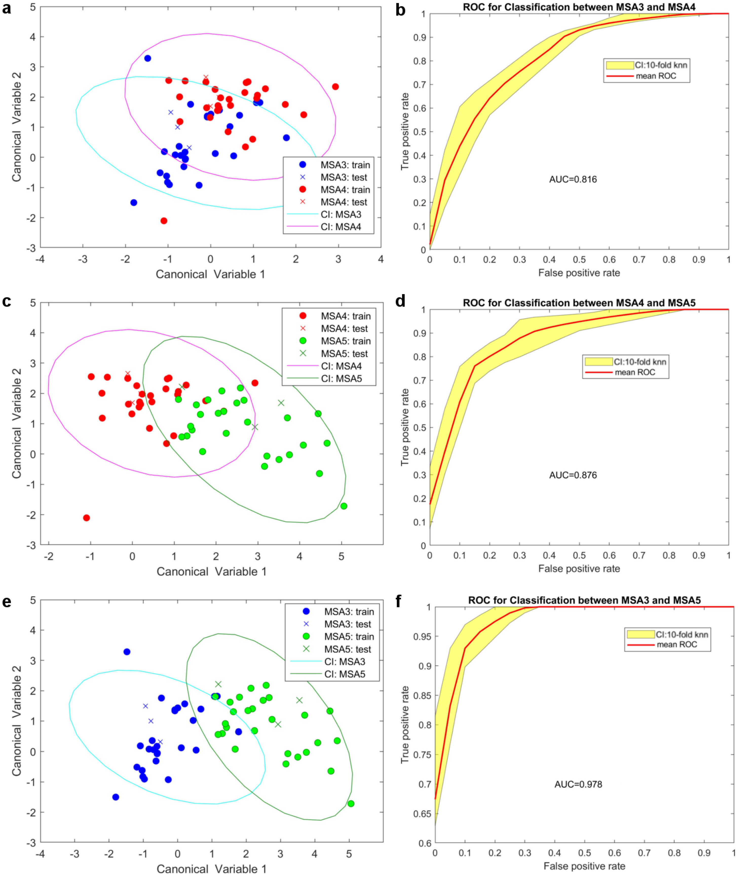
3.3. Pairwise Classification and Validation

Initially, we utilised all 33 features to evaluate binary classifier models for distinguishing between MSA grades 3 and 4, grades 4 and 5, and grades 3 and 5. We compared several binary classifiers, including decision trees, discriminant analysis, logistic regression, naive Bayes classifiers [19], kernel distributions, support vector machines [20], nearest neighbour classifiers, and ensemble classifiers [21]. Our findings indicated that the k-nearest neighbour (k-NN) classifier [22,23] provided the best results for our dataset, based on accuracy and classification error metrics for each binary classification scenario. Subsequently, we optimised the k-NN classifiers by adjusting the number of neighbours (k) and the type of k-NN classifier [24], employing a bootstrap method [25] for validation. We selected the cosine algorithm for the k-NN classifier, setting the number of neighbours to k = 7 for MSA3 vs. MSA4, k = 5 for MSA4 vs. MSA5, and k = 3 for MSA3 vs. MSA5.

For cross-validation purposes, we divided each dataset into training (90%) and test (10%) subsets [26]. This approach was applied to each binary classifier, resulting in 10 observations per classifier. We then calculated the mean ROC curve and its distribution across all combinations. Figure 3 illustrates the training and test data points for each binary classifier (shown in Figure 3a,c,e), along with the corresponding mean ROC curve and its distribution by region (shown in Figure 3b,d,f). Among the comparisons, the distinction between MSA grades 3 and 5 demonstrated the highest separation effectiveness (AUC = 0.978), compared to MSA3 vs. MSA4 (AUC = 0.816) and MSA4 vs. MSA5 (AUC = 0.876).

3.4. Feature Selection for Multi-Classifier Models and Model Tuning

For practical applications, a multi-classifier model is essential, as it is unrealistic to predict meat grades from unknown samples using only pairwise comparisons. Neighbour (k-NN) classifiers with an array of k values and employed a cosine-kNN classifier for model optimisation [24,25]. To reduce computational complexity, we focused on extracting important features with a reduced representation rather than using the full-sized input. We employed the Minimum Redundancy Maximum Relevance (MRMR) algorithm [27] to identify an array of the most critical features, aiming to optimise the model based on accuracy and classification error.

To fine-tune the classifier, we varied the number of important features from the most important feature to all 33 features, concurrently adjusting the k value from 1 to 16 to achieve the best accuracy. Figure 4a,b illustrate the accuracy and classification error for these varying parameters, respectively. Our analysis revealed that the top 10 features offered better accuracy and the lowest classification error across the range of k values (as shown in Figure 4c,d). After determining the top 10 features, we finalised our model with k = 10, adhering to the guideline that k should not exceed the square root of the number of training data points [28,29]. Although k = 9 offered similar accuracy, we decided against this value to prevent any potential voting ties [28].

3.5. Validating the Multi-Classifier Model with a Set of Blind Samples

After optimising our k-nearest neighbour classifiers (using a cosine distance, k = 10, and the top 10 features), we conducted a blind test. For this test, three samples from each grade were selected and assigned numbers in a blind manner, as depicted in Figure 5a. Images of the nine test samples were then captured using the prototype device, and the same number of features were extracted to create a blind dataset. Upon testing the accuracy of our model against this dataset, we achieved an 89% success rate, with eight out of nine samples correctly classified. The confusion matrix detailing our results for the blind dataset is shown in Figure 5b.

4. Conclusions

In this study, we designed and constructed a fluorescence-based prototype device using a 325 nm LED, a CMOS camera, and two emission filters to emulate and potentially replace the high-cost Fluoromax spectrofluorometer traditionally used for autofluorescence spectroscopy experiments. This innovation allowed for a significantly more cost-effective solution, making it accessible to small-scale meat processing industries and distributors. Using the prototype device, images were successfully captured, analysed, and subjected to a blind test on meat samples and cross-validated for various experimental settings. Our developed classification model was able to distinguish between all MSA grades with high accuracy. Moreover, this study introduces a more robust and practical approach for capturing 2D fluorescent images as opposed to the 1D data points acquired from a spectrofluorometer, indicating that low-cost autofluorescent imaging implementations could be promising alternatives for meat quality assessment.

These findings suggest that the implementation of the CMOS sensor could improve accuracy, even with a longer working or focal distance, which would be advantageous for top-mounted camera monitoring systems. Additionally, employing a simpler, feature-based classifier could increase throughput in meat processing units. The prototype device has the potential to be adapted into a handheld device with the incorporation of a shorter focal lens. Furthermore, the accuracy of data classification could be enhanced by expanding the sample collection.

References

1. Whitnall, T.; Pitts, N. Meat Consumption. 2020. Available online: https://www.agriculture.gov.au/abares/research-topics/agricultural-outlook/meat-consumption (accessed on 5 March 2021).
2. Font-i-Furnols, M.; Guerrero, L. Consumer preference, behavior and perception about meat and meat products: An overview. Meat Sci. 2014, 98, 361–371. [Google Scholar] [CrossRef] [PubMed]
3. Yates-Doerr, E. Meeting the demand for meat? Anthropol. Today 2012, 28, 11–15. [Google Scholar] [CrossRef]
4. Novaković, S.; Tomašević, I. A comparison between Warner-Bratzler shear force measurement and texture profile analysis of meat and meat products: A review. IOP Conf. Ser. Earth Environ. Sci. 2017, 85, 012063. [Google Scholar] [CrossRef]
5. Font-i-Furnols, M.; Čandek-Potokar, M.; Maltin, C.; Prevolnik Povše, M. A Handbook of Reference Methods for Meat Quality Assessment; European Cooperation in Science and Technology (COST): Brussels, Belgium, 2015. [Google Scholar]
6. Caine, W.; Aalhus, J.; Best, D.; Dugan, M.; Jeremiah, L. Relationship of texture profile analysis and Warner-Bratzler shear force with sensory characteristics of beef rib steaks. Meat Sci. 2003, 64, 333–339. [Google Scholar] [CrossRef] [PubMed]
7. Egelandsdal, B.; Wold, J.P.; Sponnich, A.; Neegård, S.; Hildrum, K.I. On attempts to measure the tenderness of Longissimus dorsi muscles using fluorescence emission spectra. Meat Sci. 2002, 60, 187–202. [Google Scholar] [CrossRef] [PubMed]
8. Islam, K.; Mahbub, S.B.; Clement, S.; Guller, A.; Anwer, A.G.; Goldys, E.M. Autofluorescence excitation-emission matrices as a quantitative tool for the assessment of meat quality. J. Biophotonics 2020, 13, e201900237. [Google Scholar] [CrossRef] [PubMed]
9. Skjervold, P.; Taylor, R.G.; Wold, J.P.; Berge, P.; Abouelkaram, S.; Culioli, J.; Dufour, E. Development of intrinsic fluorescent multispectral imagery specific for fat, connective tissue, and myofibers in meat. J. Food Sci. 2003, 68, 1161–1168. [Google Scholar] [CrossRef]
10. SádeCká, J.; TóThoVá, J. Fluorescence spectroscopy and chemometrics in the food classification—A review. Czech J. Food Sci. 2007, 25, 159. [Google Scholar] [CrossRef]
11. Australia, M.L. The effect of marbling on beef eating quality. 2018, pp. 15–16. Available online: https://www.mla.com.au/globalassets/mla-corporate/marketing-beef-and-lamb/documents/meat-standards-australia/msa-beef-tt_full-info-kit-lr.pdf (accessed on 9 April 2024).
12. Lakowicz, J.R. Principles of Fluorescence Spectroscopy; Springer Science & Business Media: Berlin/Heidelberg, Germany, 2013. [Google Scholar]
13. Bigas, M.; Cabruja, E.; Forest, J.; Salvi, J. Review of CMOS image sensors. Microelectron. J. 2006, 37, 433–451. [Google Scholar] [CrossRef]
14. Köklü, G.; Ghaye, J.; Etienne-Cummings, R.; Leblebici, Y.; De Micheli, G.; Carrara, S. Empowering low-cost cmos cameras by image processing to reach comparable results with costly ccds. BioNanoScience 2013, 3, 403–414. [Google Scholar] [CrossRef]
15. Genot, C.; Tonetti, F.; Montenay-Garestier, T.; Drapron, R. Front-face fluorescence applied to structural studies of proteins and lipid-protein interactions of visco-elastic food products. I: Designing of front-face adaptor and validity of front-face fluorescence measurements. Sci. Des Aliment. 1992, 12, 199–212. [Google Scholar]
16. Parker, C.A. Photoluminescence of Solutions: With Applications to Photochemistry and Analytical Chemistry; Elsevier Publishing Company: Amsterdam, The Netherlands, 1968. [Google Scholar]
17. Mellen, N.M.; Tuong, C.-M. Semi-automated region of interest generation for the analysis of optically recorded neuronal activity. Neuroimage 2009, 47, 1331–1340. [Google Scholar] [CrossRef] [PubMed]
18. Australia, M.S. This MLA’s Annual Report 2010–2011. (Meat & Livestock Australia, 2011). Available online: https://www.mla.com.au/globalassets/mla-corporate/generic/about-mla/anual-report-2010-11-final.pdf (accessed on 9 April 2024).
19. Ng, A.Y.; Jordan, M.I. On discriminative vs. generative classifiers: A comparison of logistic regression and naive bayes. Adv. Neural Inf. Process. Syst. 2001, 14, 841–848. [Google Scholar]
20. Cristianini, N.; Shawe-Taylor, J. An Introduction to Support Vector Machines and Other Kernel-Based Learning Methods; Cambridge University Press: Cambridge, UK, 2000. [Google Scholar]
21. Rokach, L. Ensemble-based classifiers. Artif. Intell. Rev. 2010, 33, 1–39. [Google Scholar] [CrossRef]
22. Fix, E.; Hodges, J.L. Discriminatory analysis. Nonparametric discrimination: Consistency properties. Int. Stat. Rev. /Rev. Int. De Stat. 1989, 57, 238–247. [Google Scholar] [CrossRef]
23. Altman, N.S. An introduction to kernel and nearest-neighbor nonparametric regression. Am. Stat. 1992, 46, 175–185. [Google Scholar] [CrossRef]
24. Everitt, B.S.; Landau, S.; Leese, M.; Stahl, D. Cluster Analysis; John Wiley: Hoboken, NJ, USA, 2011. [Google Scholar]
25. Hall, P.; Park, B.U.; Samworth, R.J. Choice of neighbor order in nearest-neighbor classification. Ann. Stat. 2008, 36, 2135–2152. [Google Scholar] [CrossRef]
26. Kuhn, M.; Johnson, K. Applied Predictive Modeling; Springer: Berlin/Heidelberg, Germany, 2013; Volume 26. [Google Scholar]
27. Auffarth, B.; López, M.; Cerquides, J. Comparison of redundancy and relevance measures for feature selection in tissue classification of ct images. In Industrial Conference on Data Mining; Springer: Berlin/Heidelberg, Germany, 2010; pp. 248–262. [Google Scholar]
28. Raeisi Shahraki, H.; Pourahmad, S.; Zare, N. Important neighbors: A novel approach to binary classification in high dimensional data. BioMed Res. Int. 2017, 2017, 7560807. [Google Scholar] [CrossRef] [PubMed]
29. Lantz, B. Machine Learning with R; Packt Publishing: Birmingham, UK; Mumbai, India, 2015. [Google Scholar]
Figure 1. Excitation–emission matrices (EEMs). (a) Lean meat; (b) fat reference; (c) schematic diagram for optical apparatus; and (d) prototype instrument.
Electronics 13 01623 g001
Figure 2. (ac) Each panel consists of fluorescence images from Filter 1 and Filter 2 for (a) MSA 3, (b) MSA 4, and (c) MSA 5. (df) Each panel consists of fluorescence images from Filter 2 before and after using the masking for (d) MSA 3, (e) MSA 4, and (f) MSA 5.
Electronics 13 01623 g002
Figure 3. Binary classifier model for MSA3 vs. MSA4 (a,b), MSA4 vs. MSA5 (c,d), and MSA3 vs. MSA5 (e,f).
Electronics 13 01623 g003
Figure 4. Overview of tuning parameters based on feature numbers and the kth value used in a knn-based classifier. (a) Accuracy and (b) classification error for the validated dataset. (c) accuracy and (d) class error calculation for a knn-based classifier for using 10 best features over different kth parameters.
Electronics 13 01623 g004
Figure 5. (a) Blind samples were initially marked with samples 1–9. For presentation purposes, we put the specific group number on top of the image. (b) Confusion matrix for a blind sample using our tuned classifier.
Electronics 13 01623 g005
Disclaimer/Publisher’s Note: The statements, opinions and data contained in all publications are solely those of the individual author(s) and contributor(s) and not of MDPI and/or the editor(s). MDPI and/or the editor(s) disclaim responsibility for any injury to people or property resulting from any ideas, methods, instructions or products referred to in the content.