Article

AI for Automating Data Center Operations: Model Explainability in the Data Centre Context Using Shapley Additive Explanations (SHAP)

1
School of Computer Science, University College of Dublin (UCD), D04 V1W8 Dublin, Ireland
2
ENEA-R.C. Portic, 80055 Neaples, Italy
3
ENEA-R.C. Casaccia, 00123 Rome, Italy
4
Escuela Politécnica Superior, Departamento de Ciencias de la Compuatacion, Universidad de Alcalà, 28805 Alcalá de Henares, Spain
*
Author to whom correspondence should be addressed.
Electronics 2024, 13(9), 1628; https://doi.org/10.3390/electronics13091628
Submission received: 27 February 2024 / Revised: 18 April 2024 / Accepted: 22 April 2024 / Published: 24 April 2024
(This article belongs to the Special Issue Advances in AI Engineering: Exploring Machine Learning Applications)

Abstract

:
The application of Artificial Intelligence (AI) and Machine Learning (ML) models is increasingly leveraged to automate and optimize Data Centre (DC) operations. However, the interpretability and transparency of these complex models pose critical challenges. Hence, this paper explores the Shapley Additive exPlanations (SHAP) values model explainability method for addressing and enhancing the critical interpretability and transparency challenges of predictive maintenance models. This method computes and assigns Shapley values for each feature, then quantifies and assesses their impact on the model’s output. By quantifying the contribution of each feature, SHAP values can assist DC operators in understanding the underlying reasoning behind the model’s output in order to make proactive decisions. As DC operations are dynamically changing, we additionally investigate how SHAP can capture the temporal behaviors of feature importance in the dynamic DC environment over time. We validate our approach with selected predictive models using an actual dataset from a High-Performance Computing (HPC) DC sourced from the Enea CRESCO6 cluster in Italy. The experimental analyses are formalized using summary, waterfall, force, and dependency explanations. We delve into temporal feature importance analysis to capture the features’ impact on model output over time. The results demonstrate that model explainability can improve model transparency and facilitate collaboration between DC operators and AI systems, which can enhance the operational efficiency and reliability of DCs by providing a quantitative assessment of each feature’s impact on the model’s output.

Graphical Abstract

1. Introduction

Recently, the use of AI and ML applications within data centers (DCs) as a way to automate and optimize operations has increased. As DCs evolve and scale to meet increasing demands, AI and ML models are replacing traditional heuristics and engineering solutions, and now play a critical role in modeling plant performance and improving DC efficiency. Theof These powerful technologies engage in a wide range of operational optimisation and management aspects, including energy efficiency, cooling efficiency, resource allocation, fault detection, etc., and harnessing their capabilities across multiple layers (mainly IT and cooling systems) can offer remarkable prediction accuracy [1,2,3]. However, unlike traditional heuristics and statistical models, AI and ML models often lack trustworthiness and transparency due to their “black-box” nature. This increases concern regarding the need for explainable AI (XAI), which is essential for ensuring the practical utility, understanding, reliability, and explainability of these models’ output [4,5,6].
The SHapley Additive exPlanations (SHAP) Values framework has evolved as a way to address concerns around model explainability as a critical feature attribution method for quantifying the effect of a specific feature on each prediction output. It can improve model transparency, facilitate collaboration between humans and AI systems, and promote operational reliability by quantitatively assessing each feature’s impact on the model’s output. Hence, utilizing this XAI in the DC context is essential for understanding model decisions, pinpointing influential features that affect service reliability, performing root cause analysis, enhancing performance, performing proactive maintenance, mitigating risks, fostering continuous improvement, and ensuring adherence to regulatory compliance. However, although many XAI efforts have been made in diverse domains, to the best of our knowledge no effort has yet been made in the DC context. Hence, this paper investigates SHAP values, a model-agnostic method for interpreting AI and ML models in DC contexts, by quantifying a specific operating feature’s effect on the model output. This enables DC operators to understand the model’s decisions by identifying critical features that affect its output and making predictive maintenance decisions. However, the static analysis of feature effects using SHAP may not accurately capture the dynamic nature of the DC environment, where the operating behavior changes over time and where the relevance of features can change as well. Hence, it is essential to maintain the stability of feature effects or importance in order to ensure the credibility of SHAP-based interpretations under such situations. Moreover, the intricate interplay of characteristics in predictive models, particularly in the DC setting, necessitates an in-depth understanding of how several different aspects influence prediction outcomes.
In this paper, harnessing the capabilities of the SHAP values method, we explore model interpretation and explanation in the DC context as a way to promote transparency and trust-building in the use of AI and ML models. To capture the temporal feature relevance over time in the dynamic environment, we perform Temporal SHAP Values (TSHAPV) analysis by taking 15 min of data and capturing the importance of the temporal features’ impact on the predictive model. This is based on the previous temporal foundation put forward by [7,8,9]. Our study begins with background applications of AI and ML models in DCs, the theoretical foundations of XAI, and their applicability, which are discussed in Section 2 below. This is followed by a discussion of data collection and preprocessing, selected model building, and finally the theoretical foundations of SHAP and its applicability in the DC context in Section 3.3. Next, Section 4 presents expected limitations when SHAP is applied in the DC context. The results of our experimental analysis are presented in Section 5. Finally, we present our conclusions and prospects for future work. Our approach is demonstrated through selected RF, XGB, and LSTM-based DC ambient temperature predictions. This comprehensive approach provides an informed understanding of SHAP’s pivotal role in enhancing the interpretability and trustworthiness of predictive models, particularly in the DC environment. We validated our proposed approach using a historical dataset from an HPC DC sourced from Enea CRESCO6 cluster operations data, which are monitored every 15 min and contain 54 features.
Our contributions in this paper are as follows: (1) we apply the SHAP values XAI method to interpret AI and ML predictive models in the DC context as a way to improve transparency and trustworthiness. SHAP quantifies the effect of each feature on the model output, enabling DC operators to understand the operation’s impacting features and make informed predictive maintenance decisions. This method can help to facilitate collaboration between DC operators and AI systems, enhancing DC operational efficiency and reliability by quantitatively assessing each feature’s impact on the model’s output. (2) We explore feature interactions and their impact on the predictive model output, which we demonstrate using the dependency explanation tool. DC operators can gain insights into how different features influence each other and impact the model’s predictions. This understanding can help operators to interpret the model’s behavior, identify essential features, and improve the model’s performance. (3) We explore the relevance of temporal features in the dynamic environment over time using Temporal SHAP (TSHAP), which allows a typical feature’s impact on model output over time to be assessed.

2. Related Work

In this section, we briefly discuss the applications of AI and ML models to optimize DC operations and the applicability of XAI to interpret these models. DCs are the backbone of ever-increasing economic activities, enabling system operations, data storage, and networking capabilities in a reliable and scalable fashion [10]. DCs are evolving and scaling to meet increasing demands. Due to increasing physical complexity, the sheer number of possible configurations, plant performance, nonlinear system interactions, and the need to monitor enormous amounts of operations management data from various aspects of operations, optimizing a typical DC operation presents challenges that cannot be addressed using traditional rule-based and engineering solutions. Recently, DCs have been able to realize significantly increased performance, efficiency, and reliability by harnessing the power of AI and ML models. For instance, utilizing a simple Neural Network (NN) ML approach, Google was able to reduce cooling costs by 40% by predicting power usage effectiveness and adjusting controllable parameters [1]. Research by Bianchini, R. et al. has implemented an XGB tree-based model for efficient resource and workload management towards ml-centric cloud platforms [2]. Other efforts include research by Haghshenas et al. [3] that utilized a multi-agent machine learning (ML) strategy for energy-efficient virtual server consolidation and a study by Z. Yang et al. [11] that implemented a light gradient boosting machine, a recurrent neural network, and random forests to optimize the energy efficiency of the total input energy per year of a DC by 0.24%. Another study [12,13] utilized machine learning thermal modeling to enhance DC energy efficiency, and many more efforts have been implemented to automate and optimize DC operations.
As discussed above and indicated elsewhere in the literature, AI and ML techniques are ideal solutions for automating and optimizing DC operations with high accuracy. However, unlike traditional heuristics and statistical models, interpreting these black-box AI and ML models is challenging and represents a significant concern. Hence, incorporating XAI approaches has become paramount as a way to ensure that advances in ML models remain explainable and transparent [14,15,16]. XAI strives to encompass particular motivations, such as accountability, fairness, privacy, reliability, transparency, and trust-building [17], in order to ensure the overarching goal of applying AI and ML technologies [18]. Although efforts have been made in diverse domains, including complex systems analysis, to the best of our knowledge no such efforts have been made in the DC context. The most popular XAI methods are LIME [19], DeepLIFT [20], Layer-Wise Relevance Propagation (LRP) [21], classical Shapley values [22], and SHAP [23], which includes different versions such as TreeSHAP [24] and DeepSHAP [23]. More details about these approaches can be found in [25]. In the context of time series problems, which is similar to the DC context, there are efforts such as [26,27], which utilized SHAP and LIME, respectively, for time series classification, focusing on global feature attribution-based explanations. Efforts have been applied to time series forecasting; for instance, the research by [28] utilized LIME and SHAP for time series forecasting, and [29] utilized time series SHAP (TsSHAP) to provide explanations of univariate time series forecasting models. In [30], the authors provided detailed evaluations of the popular LIM, LRP, and SHAP explainers. In addition to SHAP’s good missingness, consistency, and accuracy properties, the authors ranked SHAP as the most reliable, while the other approaches were biased towards specific model architectures. Furthermore, SHAP values have gained considerable interest compared to other XAI approaches because of their distinctive combination of accuracy and interpretability [31]. SHAP can offer a reliable and essential way to determine the significance of features, which is extremely helpful in quantifying a specific feature in a complex environment such as DC. According to the literature, SHAP has emerged to bridge the gap between model accuracy and transparency, making it more trustworthy. With all of these justifications, the present paper adopts SHAP to interpret AI and ML models in the DC context.
While SHAP’s contributions to explaining predictive modeling are substantial, several gaps remain. Most notably, existing works have often overlooked temporal changes in feature importance and the complex interactions between them [32,33,34]. Further, although methodologies such as time series and survival analysis have provided invaluable insights [35,36,37], capturing temporal issues has not been considered essential. In this paper, we adopt model explainability using SHAP and explore its application in the DC context. We additionally address temporal capture challenges using sensitivity analysis and observing the model’s behavior over time, aiming to achieve a deeper understanding of feature collaborations over time. As SHAP values have already gained prominence for their robust mathematical grounding and versatility across models [38,39,40], the distinguishing aspect of this research is its focus on model interpretability in the DC context. With the growing implementation of AI and ML models, understanding their decision-making process and ensuring their transparency is critical to improving trustworthiness in industry. The proposed methodology maintains a high level of prediction accuracy and provides valuable insights into the features that most impact the predictive process.

3. Methodology

As illustrated in Figure 1, this section details AI and ML model explainability and interpretation implementation using SHAP on commonly used RF, XGB, and NN prediction models to demonstrate the explainability of XAI in the DC context. As indicated in Figure 1, the method consists of the following four steps: (i) data collection and preprocessing, including data preprocessing, feature engineering, and relevant input feature selection, splitting dataset into 80% for training and 20% for testing; (ii) model building and hyperparameter configuration, and trained the specified model using 80% of the training data; (iii) describing the theoretical foundations of SHAP explainer and applied to any of the trained models; and (iv) then presented the model interpretation and explanation results (applying SHAP on the training and testing data not changed the feature importance).

3.1. Dataset and Preprocessing

This paper uses data from the ENEA CRESCO6 cluster, consisting of 434 computing nodes with 20,832 cores and operating parameters monitored by onboard sensors. The cooling system’s operating parameters, including supply air, return air, relative humidity, airflow, fan speed, etc., are monitored using the cooling machine’s onboard sensors. Environmental conditions are monitored using smart sensors installed around the cluster. These data streams are accessed through an intelligent platform management interface (IPMI), and stored in three MySQL database tables. The datasets were recorded in three tables for the energy and workload, cooling system, and environmental conditions-related parameters. Table 1 illustrates the collected raw data, which were monitored over a range of seconds and minutes.
Hence, following data collection, we performed data preprocessing tasks with expert consultation to ensure high-quality data for AI and ML models. Irrelevant features were removed from each table. For example, in each table, there were two time stamps, one of which was machine-readable and the other actual human-understandable; we removed one and used the other as an index for each table. The datasets were then reshaped into (34,553.24), (34,553.6), and (34,553.20), into 15 minute equal time resolutions, and aggregated into a single compact dataset at the DC level reshaped as (34,553.50). This DC operational dataset was treated as a multivariate time-series problem. In such problems, temporal or covariate feature considerations are essential to understanding the temporal behavior of the data. For instance, DC ambient temperature behavior changes at different time scales, such as hours, days, etc. Hence, we used feature engineering to extract time-based covariate features, which have significant predictive power for the target variable. Based on that, we identified four features extracted as temporal features, i.e., hours, days, months, and quarters. Finally, the dataset used in this paper was reshaped as (34,553.54), that is, 34,553 instances and 54 features. The list of input features and descriptions is provided in Appendix A.
However, as some of the data may not be relevant to effectively model the target variable (in this case, DC ambient temperature), we used the SHAP-assisted feature selection method from our previous paper [41] to identify relevant features. Next, we performed data normalisation, also known as feature scaling, which is recommended due to the wide range of raw feature values. The values of a feature vector z were mapped to the range [−1, 1] by:
z n o r m = z m e a n ( z ) / m a x ( z ) m i n ( z ) .
We validated the performance of the selected prediction models using the Mean Squared Error (MSE), Root Mean Square Error (RMSE), and Mean Absolute Error (MAE) metrics.

3.2. Prediction Models

Data-driven models based on AI and ML emphasize learning patterns and relationships directly from the dataset without relying on explicit knowledge. These empirical algorithms rely on observed data to capture flexible patterns and relationships, which can be adapted to model and optimize DC operations without extensive domain knowledge. This section presents the description, architecture, and hyperparameter configurations of the selected RF, XGB, and LSTM DC ambient temperature prediction models to be explained.

3.2.1. Random Forest Forecasting

A random forest (RF)-based DC ambient temperature prediction model was established to forecast every 15 min. RF was initially proposed by Ho (1995) [42] and further updated by L.Breiman [43], and is now a widely used method in regression and classification problems. RF regression is an average prediction across the decision trees in time-series forecasting. Before fitting the model, we transformed the data into a supervised learning approach using the shift function Python module. For instance, for a target variable y, its lag_time is provided as y t 1 , y t and y t + 1 . In this case, y t 1 and y t are the lagged time of y t and y t + 1 , respectively. Note that the lag_time is used to create features that capture the relationship between a time series’ past values and its current ones. Then, we fitted the model and validated it using a walk-forward validation approach. The training dataset was utilized to identify the optimal parameters for the random forest model, while the testing dataset was exclusively used to validate the model’s prediction quality. The optimal hyperparameters used in this paper were tuned as shown in Table 2.

3.2.2. XGBoost

A more robust machine learning model than RF, XGBoost (XGB) was also used to forecast the DC ambient temperature. XGB is an optimized gradient boosting decision tree (GBDT) algorithm widely used in classification and regression problems [44]. In XGBoost regression, the average prediction across the decision trees is used to forecast the DC ambient temperature. As in RF, we transformed the data into a supervised learning approach using the shift function before fitting the model. The model was validated using a walk-forward validation approach. The training dataset was utilized to identify the optimal parameters for the XGB, while the testing dataset was exclusively used to validate the model’s prediction quality. The model was implemented using the sklearn package. The optimal hyperparameters used in this paper were tuned as shown in Table 3.

3.2.3. Long Short-Term Memory (LSTM) Deep Learning

In addition, we developed an LSTM-based DC ambient temperature prediction model. LSTM is a popular Recurrent Neural Network (RNN) introduced by Schmidhuber et al. in 1997 [45] for sequential data analysis. LSTM overcomes the vanishing and exploding gradient limitations of RNNs by introducing four modules with internal memory control. The LSTM modules consist of internal memory, a forget gate, an input gate, and an output gate. As illustrated in Figure 2, the memory component tracks input sequence dependencies, while the gates control the LSTM’s ability to remove or add information. The forget gate determines the time a value remaining in the cell. The LSTM memory unit follows Equations (2)–(7).
f t = σ w f h t 1 , x t + b f
i t = σ w i h t 1 , x t + b i
c ˜ t = t a n h w c h t 1 , x t b c
c t = f t c t 1 + i t c ˜ t
o t = σ w o h t 1 , x t + b o
h t = o t tan h C t
As Equation (1) indicates, f t is the forget gate range of (0, 1), w f is the weight, and b f is the bias value applied to the forget gate, while x t is the input feature of the current time t and h t 1 is the output value of the last moment. In Equations (2) and (3), i t is the input gate with a value range of (0, 1), w i is the weight, b i is the bias of the input gate, w c is the weight of the candidate input gate ( c ˜ t ), and b c is the bias of the candidate input gate. In Equation (5), c t is within the range of (0, 1). In Equation (6), o t is within the range of (0, 1), w o is the weight of the output gate, and b o is the bias of the output gate. In Equation (7), h t determines the information that should be passed to the next sequence. We implemented a four-layer LSTM model consisting of an input layer, two hidden layers, and one output layer. Table 4 provides the implemented LSTM architecture hyperparameter settings. The input included 54 features, 64 neurons, and 10 time steps or window_size.

3.3. Theoretical Foundations of the Shapley Additive Explanations (SHAP) Method

As illustrated in Figure 1, this paper uses the SHAP values method to interpret the output of AI and ML models. SHAP provides a feature-based explanation ϕ R d , where d is a dimension vector representing each feature’s contribution score for the corresponding feature. In addition to its missingness, consistency, and accuracy, SHAP is a human institution method [23] with advanced performance, outperforming other explainers in the literature. It quantifies the impact of a specific feature on a prediction model for specific instances [23]. It bridges the gap between a trained model’s accuracy and interpretability. The critical principle involves calculating each feature’s contribution to the prediction by considering all possible feature combinations. This entails assessing the difference in prediction when including and excluding a feature (as calculated in Equation (8)) while considering all possible combinations of other features. This comprehensive approach guarantees a fair assessment of each feature’s contribution within the context of all other features. The SHAP values methodology is detailed in Molnar (2020) [25], and a more intuitive introduction is provided by Mazzanti (2020) [46,47]. The Shapley values for each feature are calculated by Equation (8):
S H A P ( ϕ i ) = S N { i } | S | ! ( N | S | 1 ) ! N ! [ v ( S { i } ) v ( S ) ]
where ϕ i the contribution of feature i, N is the set of all features, S is a subset of features | S | that denotes the size of the set, v ( S { i } ) is the prediction with both the features in set and feature, and v ( S ) is the prediction with just the features in set S. As illustrated in Equation (8), the contribution of feature i is computed by iterating over all possible subsets S of the remaining features in N and comparing the difference in the prediction when feature i is included versus when it is excluded.
In contrast to more straightforward techniques such as LIM, SHAP profoundly determines the direction and size of each feature’s impact, which is crucial for comprehending complex models. Thanks to its theoretical basis in cooperative game theory, interpretations are guaranteed to be consistent and dependable. The approach performs exceptionally well at capturing complex interactions and nonlinear correlations between features, which is an essential component of advanced ML models. As SHAP is model-agnostic, it can be used with a wide range of models, including deep neural networks and simple regressions. It is crucial for in-depth instance-level comprehension and more comprehensive model behavior analysis, as it provides both local and global insights. This viewpoint improves a model’s transparency and reliability, which is particularly important in delicate domains such as the DC environment. Moreover, SHAP assists in the process of feature engineering and model refining, enabling the development of models that are both more efficient and easier to interpret, which functions as a conduit providing lucidity and responsibility to complex machine learning forecasts, rendering it an essential instrument in the realm of AI and machine learning technologies. This paper uses the TreeSHAP explainer for the tree-based models (RF and XGB) and DeepSHAP for the deep learning model (LSTM).

4. Limitations

Although the SHAP explainer can provide insightful information about the black-box machine learning models in the DC context, there are several issues to consider when implementing SHAP explanations which may limit their use in the context of data centers:
  • Data Quality and Variability: Inconsistency, noise, and missing values in data can all impact the reliability of SHAP explanations in the DC context. The stability and consistency of SHAP values can be impacted by variations in data center environments over time, such as shifts in workload patterns, hardware configurations, or environmental factors.
  • Real-time Interpretability: Many data center applications require real-time decision-making in response to events or situations that change over time. The processing expense of computing SHAP values may make generating SHAP explanations for predictions in real-time impractical, particularly for complicated models such as deep learning or for enormous data sets.
  • Domain Expertise Requirement: Understanding the significance of features, interpreting the direction and size of feature contributions, and making defensible decisions based on the information provided by SHAP values when interpreting SHAP explanations may require domain expertise. In data center operations, it can be challenging to bridge the knowledge gap between domain-specific experience and data science competence.

5. Experimental Results

This section illustrates the experimental performance analysis of the predictive models presented in Section 5.1, Table 5 and the experimental analysis for black-box model ML explanations formalised starting from Section 5.2.

5.1. Model Performance and Time Complexity Index

The model performance results illustrated in Table 5 are based on the optimally selected features in our previous feature selection work [41]. However, this paper’s main intention is to assess these models’ explainability. Hence, the analysis of the results focuses on model interpretation, as detailed in the following subsections.

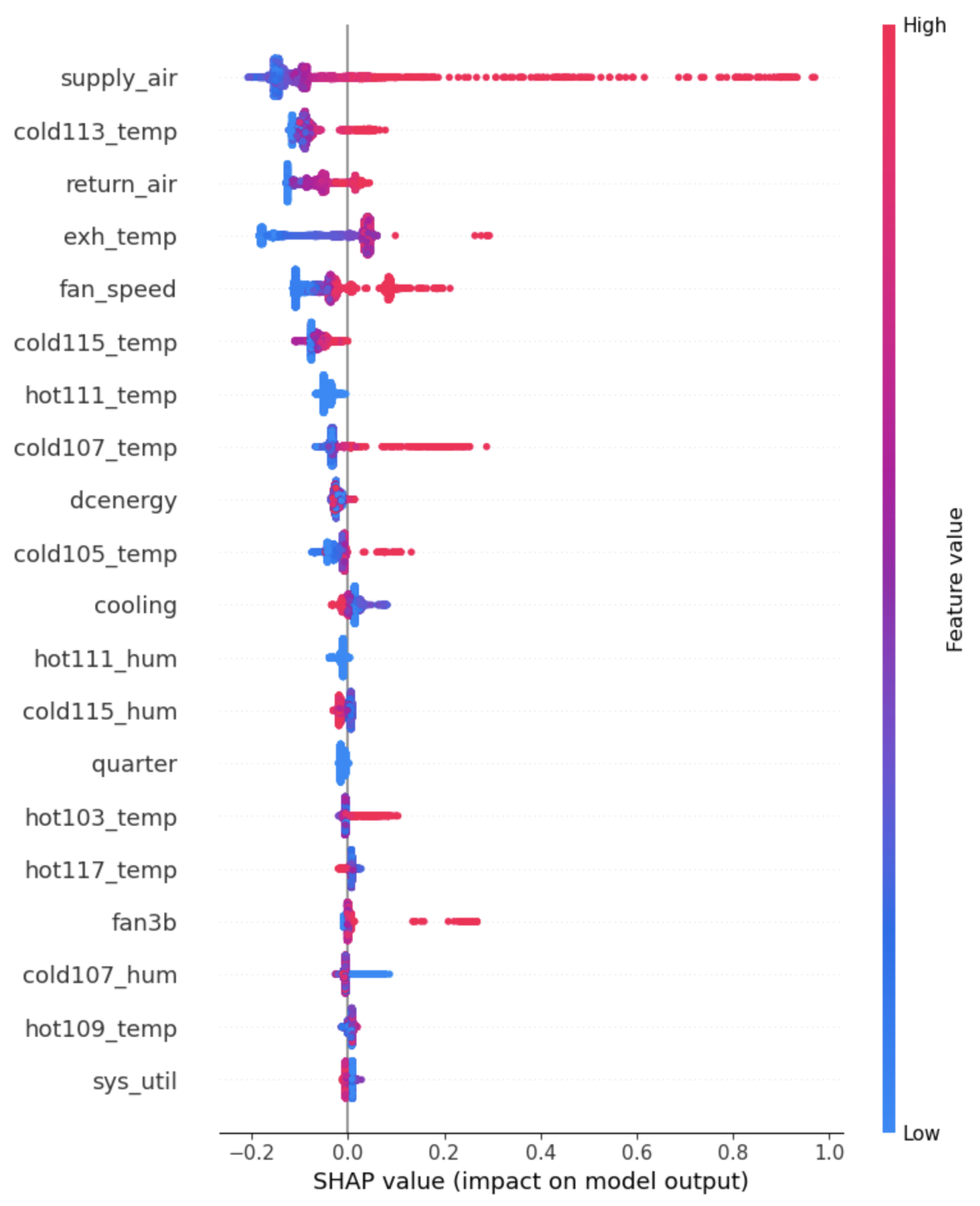
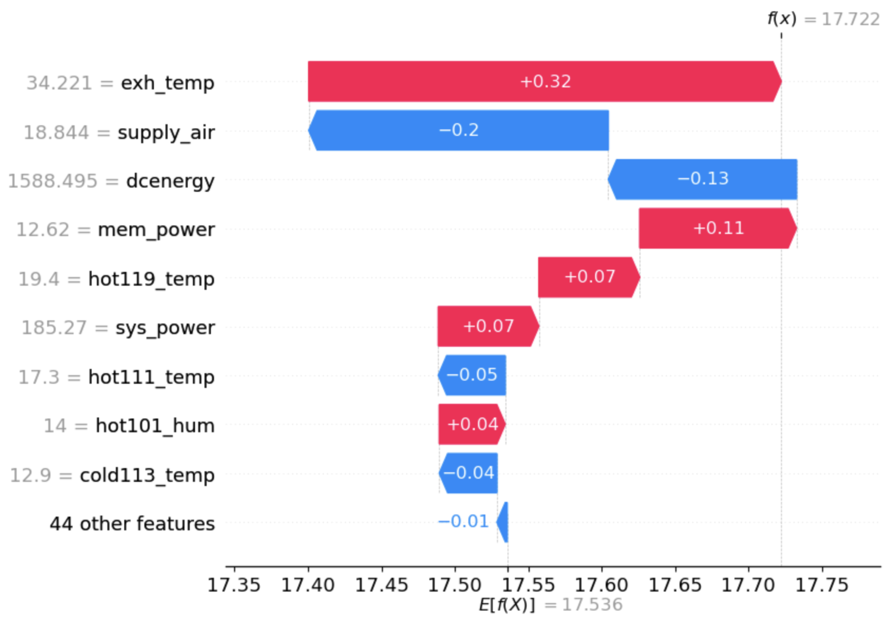
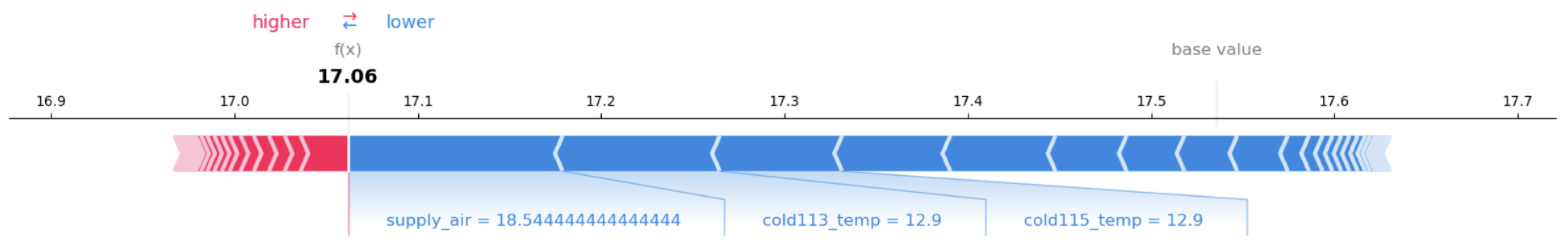
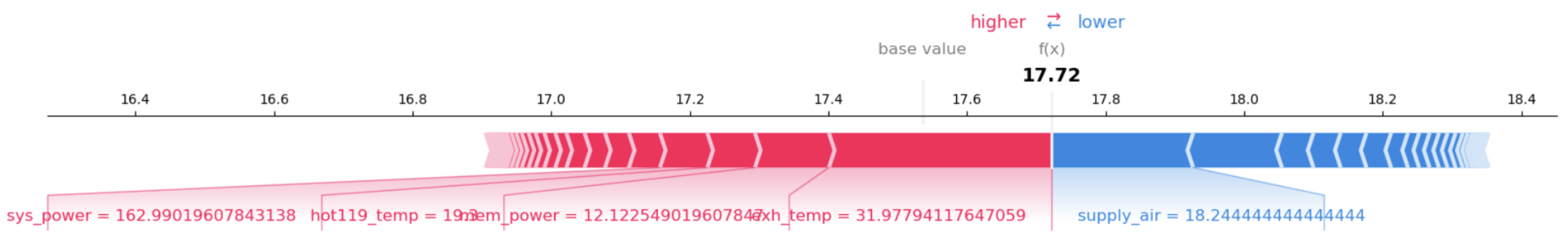
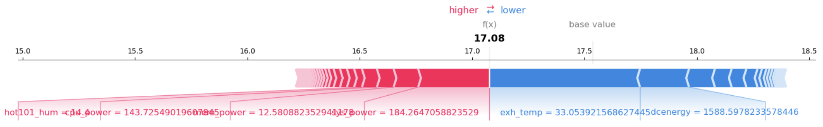
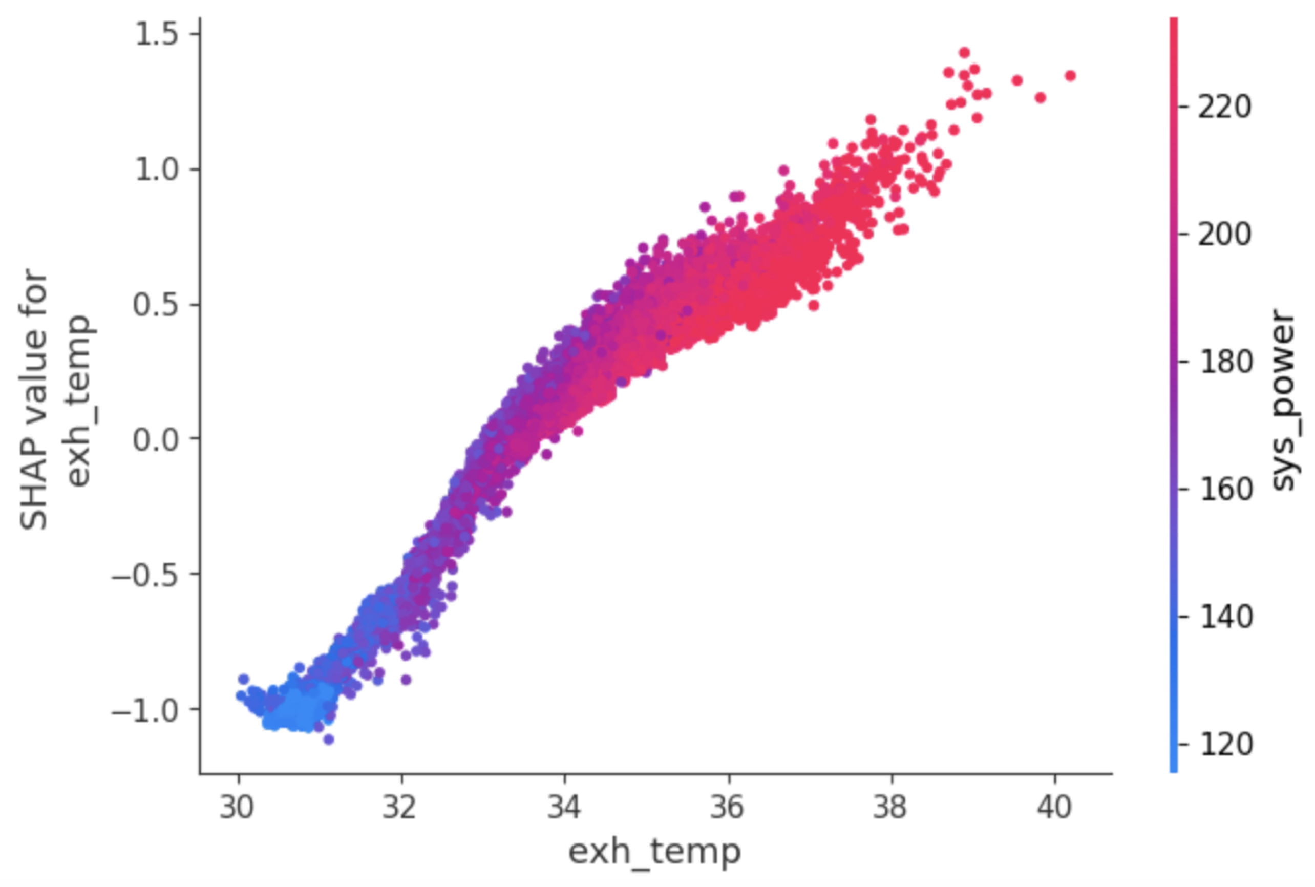
5.2. SHAP-Based Feature Importance and Comparison Analysis 

This subsection illustrates ML black-box model explanations using the SHAP method. TreeSHAP is used to interpret the tree-based ML models, while DeepSHAP is used for the deep learning model. The results were formalized using the summary, waterfall, force, and dependency explanation tools. Further, the importance of temporal features was explored in order to evaluate the method’s reliability within the dynamically changing DC environment over time. Feature importance is a cornerstone for quantifying and understanding the relative impact of features in complex machine learning models. For instance, as illustrated in Figure 3 and Figure 4, the summary plots merge the importance of features with their effects, highlighting the features’ global importance [48]. Each point on the summary plot represents a Shapley value for various DC ambient temperature prediction features. Figure 3 and Figure 4 illustrate that the features displayed on the y and x axes determine the Shapley value. The color denotes each feature’s value, which ranges from low (blue) to high (red). The x axis indicates a positive value, while red color denotes a high value. The features are vertically ordered by their shape values and average importance to the predictions [19]. The distribution of the Shapley values for each feature can be ascertained by examining the overlapping points that exhibit jittering along the y axis direction. It can be seen in Figure 3 and Figure 4 that exh_temp and supply_air have the most significant impacts on the ambient temperature. The analyses shown in Figure 3 and Figure 4 reveal that certain features, specifically supply_air and exh_temp, consistently emerge as highly important across the DC ambient temperature predictions. However, the SHAP value for any given feature is not constant, and varies from phase to another in this dynamic environment over time. This variability highlights the importance of the measurement feature over time or across different operational phases in a dynamically changing environment. As SHAP values are the result of unique features that are particular to each prediction, we further explore waterfall, force, and dependency plots, which are essential to understanding the models in every DC ambient temperature prediction. Figure 5, Figure 6 and Figure 7 depict a waterfall plot for DC ambient temperature prediction at a specific instance, which is designed to explain individual predictions. The waterfall displays target values on the x-axis, with x representing the selected target, f ( x ) representing the model’s predicted value, and E [ f ( x ) ] representing the expected value.
As illustrated in the waterfall Figure 5, Figure 6 and Figure 7, the negative values correlate negatively with the DC ambient temperature target variable, whereas the positive values reflect a direct relationship to the model’s output. The waterfall explanation provides a comprehensive breakdown of individual features’ contributions to a specific prediction, illustrating their cumulative impact and providing a detailed understanding of individual feature contributions. The waterfall explanation indicates the contribution of each feature to prediction, with positive (+) indicating increased output and negative (−) indicating decreased output from the baseline. As illustrated in Figure 5, Figure 6 and Figure 7, supply_air, exh_temp, and supply_air were the top infrared features for a specific DC ambient temperature prediction when using RF, XGB, and LSTM, respectively. As illustrated in Figure 5, supply_air, cold113_temp, and cold115_temp push down the model output, with −0.12, −0.09, and −0.07, respectively. Similarly, the waterfall plots for XGB and LSTM are illustrated in Figure 6 and Figure 7, respectively. From a technical point of view, this explanation demonstrates to DC operators which features positively or negatively affect the DC ambient temperature, enabling them to take appropriate maintenance actions.
Figure 8, Figure 9 and Figure 10 illustrate local model interpretation for RF, XGB, and LSTM, respectively. The local explanation is based on a single instance of the data-point. Unlike the tree-based models, LSTM takes three dimensions (sequences, time steps, and input features) as input, making it challenging to apply SHAP directly to the model output. To resolve this issue, the LSTM model output flattened into two dimensions and reduced the dimensionality to the original feature size, then applied the DeepSHAP explainer to interpret this complex model. Due to increased monitoring of operations data, predictive maintenance in the DC operating environment has evolved to leverage advanced deep learning models, providing advanced operating insights into the operational efficiency and reliability of DCs.
Interpreting models using SHAP dependency plots is pivotal, as they demonstrate the relationship between model features and their impact on predictive outputs, which is essential to the predictive maintenance evolution of the DC operating temperature. Below, we explore the implications of the analytical insights derived from the SHAP dependency plots for supply_air vs. exh_temp, supply_air vs. sys_power, and exh_temp vs. sys_power, illustrated in Figure 11, Figure 12 and Figure 13, respectively, along with their translation into practical strategies for DC operating temperature maintenance.
According to the illustration in Figure 11, the SHAP plot for supply_air vs. exh_temp illustrates a positive correlation between the DC exhaust temperature (exh_temp) and the model’s ambient temperature prediction, suggesting that higher exh_temp values can signal increasing DC ambient temperature. Correcting supply_air under various operational conditions can vary the impact of exh_temp on the DC operating temperature. A practical implication is that such insights can inform maintenance strategies, promoting early inspections and interventions to maintain the DC ambient temperature when the exh_temp is higher. For instance, DC operators can maintain the ambient temperature by adjusting cooling system settings, enabling them to enhance the DC’s efficiency and service reliability.
The dependency analysis of supply_air vs. sys_power in Figure 12 shows that lower SHAP values are associated with higher air supply (supply_air), suggesting that the DC operations may be under stress related to the air supply. This allows for more targeted air supply fan maintenance based on the cooling systems of the DC, which enables maintenance of the DC operating temperature to enhance DC efficiency. In this case, the air supply negatively impacts the ambient temperature. Furthermore, as illustrated in the plot of exh_temp vs. sys_power in Figure 13, an increase in exh_temp at the DC corresponds with higher SHAP values, underscoring its importance in DC efficiency. The color gradient with sys_power indicates an interplay between exh_temp and sys_power that affects DC ambient temperature predictions. A practical implication is that regularly maintaining the DC’s ambient temperature is essential to maintaining and improving DC efficiency. Hence, the SHAP dependency plot is an excellent analytical exploration tool for interpreting black-box models.

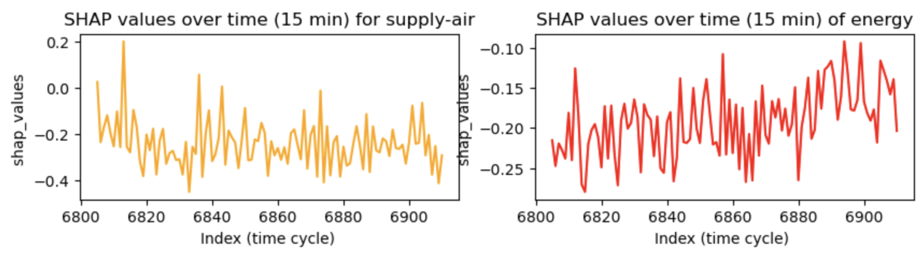
5.3. SHAP-Based Temporal Feature Importance Analysis

Unlike the traditional SHAP method, which views feature importance as a static property, mean absolute temporal SHAP (TSHAP) values are a novel evaluation metric that allows the temporal behavior of features to be captured in dynamic industrial contexts. This metric provides a reliable way to understand how features contribute to predictive models over time, particularly within the context of DCs. To demonstrate how the temporal changes of features behave over time, we used the last 15 min of data by taking the topmost essential features of each model and examining how the temporal changes are affected over time. The results of this analysis for each model concerning the topmost important features are shown in Figure 14, Figure 15 and Figure 16. We examined the SHAP values over each feature’s continuous operational time over 15 min. Figure 14, Figure 15 and Figure 16 show the SHAP values of specific features and how they behave over 15 min for the RF, XGB, and LSTM model-based DC ambient temperature predictions. This approach provides a dynamic interpretation of feature significance that enhances the more general patterns seen over time. For example, as illustrated in Figure 14, there is noticeable temporal variation in SHAP values for essential features such as cold113_temp and supply_air, which suggests that these features had different effects on the RF model’s predictions over 15 min. Similarly, as illustrated in Figure 15, there is noticeable temporal variation in the SHAP values for essential features such as exh_temp and supply_air, which suggests that these features had different effects on the XGB model’s predictions over 15 min. Finally, Figure 16 illustrates noticeable temporal variation in the SHAP values for essential features such as supply_air and energy, which suggests that these features had different effects on the LSTM model’s predictions over 15 min.
These results show that SHAP is resilient in capturing the temporal effects of any machine learning model output. It consistently captures the prediction output’s features and temporal effects, enabling DC operators to understand the output and take informed predictive maintenance actions.

6. Conclusions and Future Works

This paper makes significant and decisive steps towards enhancing the interpretability and explainability of complex AI and ML models, particularly within the DC context, using the SHAP (Shapley Additive exPlanations) method. The experimental SHAP-based explanation analysis formalizes the explanation output at the global and local levels. Delving into the interpretations of SHAP explainer tools can enhance DC efficiency and service reliability and serve as the foundation for predictive operational maintenance methods. By harnessing these analytical insights, DC operators can understand the factors that are most impactful on the models in order perform appropriate proactive maintenance actions. Our formal experimental analysis uses summary plots for global feature impact analysis, waterfall and force plots for local and global prediction, and dependency plots to capture feature interactions, providing insights into the cooperative interplay among features and how they collectively influence DC ambient temperature prediction. Our experimental analysis results for the SHAP-based model explanations are illustrated in Figure 3, Figure 4, Figure 5, Figure 6, Figure 7, Figure 8, Figure 9, Figure 10, Figure 11, Figure 12 and Figure 13. In addition, this paper delves into temporal SHAP (TSHAP), used as a foundation to reveal the temporal changes of feature importance over time. This approach offers thorough data and comprehension of features’ contributions to model predictions over time. As illustrated in Figure 14, Figure 15 and Figure 16, observing the fluctuations in the SHAP values of a specific feature over time can indicate how that particular feature behaves in the given time cycle with different prediction models. By capturing the temporal behaviors of feature importance, the approach described in this paper can inform predictive maintenance for DC operating temperatures while improving DC efficiency and reliability. By leveraging the SHAP model explanation method, operators can move towards more transparent, interpretable, and predictive maintenance while improving efficiency and operational optimizations. The interpretation of SHAP values presents a challenge in complex and dynamic environments with nonlinear configurations.
Hence, this paper constitutes a comprehensive exploration of AI and ML model interpretation based on SHAP values in the DC context, exploring feature interactions and the temporally changing impacts of features on different prediction models over time. This study can provide the DC industry with more accurate, dependable, and interpretive models by utilizing SHAP values and closely analyzing their subtleties. In addition to making a substantial contribution to the academic debate, these findings have practical implications for improving predictive maintenance strategies in the data center industry. However, even though our study has made initial initiatives towards interpreting AI and ML models in complex DC environments, it is important to acknowledge that there may be challenges around data quality and variability, real-time interpretability, and the need for intensive domain expertise. Continuous monitoring and auditing of AI and ML models in data centers involves additional challenges such as tracking performance, recalibrating explanations, and ensuring alignment with operational objectives over time.
Future studies may concentrate on resolving the discrepancies that have been found in this study and developing novel model explainability approaches for greater precision and broader application in the DC setting. To ensure that the feature importance and interactions captured by the models closely correlate with industry-specific knowledge and real-world experiences, close collaboration with DC domain experts is necessary in order to design more effective SHAP-based techniques. Another significant focus of our future work involves the robustness of SHAP values, specifically, how they behave when there are outliers and operational disruptions. We acknowledge that the current scope has its limitations, even though our findings have shown a degree of stability in these values across the analysed scenarios. Extensive validation over a larger range of operational data and quality situations and model designs is required for comprehensive robustness analysis, which is beyond the scope of present work. In light of this, we emphasize the significance of carrying out further research on the resilience of interpretability approaches such as SHAP in order to guarantee that the insights they offer continue to be trustworthy, instructive, and in line with real-time interpretation in varying circumstances.

Author Contributions

Conceptualization, methodology design, experimentation and analysis, and writing the paper: Y.G.; supervision, editing and reviewing: D.D.; editing and reviewing: D.D.C., reshaping, editing, and reviewing the paper: M.C.; reviewing: A.C. All authors have read and agreed to the published version of the manuscript.

Funding

This paper received funding from the European Union’s Horizon 2020 research and innovation program under the Marie Skłodowska-Curie grant agreement No. 778196. However, the contents of the paper reflect only the authors’ views, and the Agency is not responsible for any use that may be made of the information it contains.

Data Availability Statement

Data will be made available on request.

Conflicts of Interest

The author’s declare no conflicts of interest.

Abbreviations

The following abbreviations are used in this manuscript:
AIArtificial Intelligence
DCData Center
DCIMData Center Infrastructure Management
CNNConvolutional Neural Network
LSTMLong Short-Term Memory
RFRandom Forest
RNNRecurrent Neural Network
SHAPSHapley Additive exPlanations
MLMachine Learning
NNNeural Network
MTSMultivariate Time Series
HPCHigh-Performance Computing
XGBXGBoost
XAIExplainable AI

Appendix A

This section provides supplementary information related to the input features.
  • Timestamp_measure: the datetime for reading data streams from sensors (minutes)
  • sys_power: the total instantaneous power of each node (Watts)
  • cpu_power: the instantaneous CPU power of each node (Watts)
  • mem_power: each node’s RAM memory instantaneous power (Watts)
  • fan1a: the node’s fan speed, expressed in RPM (revolutions per minute)
  • fan1b: speed of the fan (Fan1b) installed in the node, expressed in RPM
  • fan2a: speed of the fan (Fan2a) installed in the node, expressed in RPM
  • fan2b: speed of the fan (Fan2b) installed in the node, expressed in RPM
  • fan3a: speed of the fan (Fan3a) installed in the node, expressed in RPM
  • fan3b: speed of the fan (Fan3b) installed in the node, expressed in RPM
  • fan4a: speed of the fan (Fan4a) installed in the node, expressed in RPM
  • fan4b: speed of the fan (Fan4b) installed in the node, expressed in RPM
  • fan5a: speed the fan (Fan5a) installed in the node, expressed in RPM
  • fan5b: speed of the fan (Fan5b) installed in the node, expressed in RPM
  • sys_util: the system usage (%)
  • cpu_util: the CPU usage (%)
  • mem_util: the RAM usage (%)
  • io_util: the node’s I/O traffic
  • cpu1_Temp: the CPU (CPU1) temperature (°C)
  • cpu2_Temp: the CPU (CPU2) temperature (°C)
  • sysairflow: the airflow of the node in CFM (cubic feet to minute)
  • exh_temp: the exhaust temperature (air exit of the node), expressed in °C
  • amb_temp: ambient temperature/room temperature, expressed in °C (target variable)
  • dcenergy: the DC energy demand, expressed in Kwh (target variable)
  • supply_air: the cold air or inlet temperature (°C)
  • return_air: the heat or warm air ejected to the outside (°C)
  • relative_umidity: the working humidity of the CRAC (°C)
  • fan_speed: the speed of the CRAC cooling system (RPM)
  • cooling: the working intensity of the CRAC (%)
  • free_cooling: not applicable, as all values are 0
  • hot103_temp: the hot temperature (°C) monitored by sensor hot103
  • hot103_hum: hot_humidity monitored by sensor hot103
  • hot101_temp: hot temperature (°C) monitored by sensor hot101
  • hot101_hum: hot_humidity (%) monitored by sensor hot101
  • hot111_temp: hot temperature (°C) monitored by sensor hot111
  • hot111_hum: hot_humidity (%) monitored by sensor hot111
  • hot117_temp: hot temperature (°C) monitored by sensor hot117
  • hot117_hum: hot_humidity (%) monitored by sensor hot117
  • hot109_temp: temperature (°C) monitored by sensor hot109
  • hot109_hum: hot_humidity (%) monitored by sensor hot109
  • hot119_temp: hot_temperature (°C) monitored by sensor hot119
  • hot119_hum: hot_humidity (%) monitored by sensor hot119
  • cold107_temp: cold_temperature (°C) monitored by sensor cold107
  • cold107_hum: cold_humidity (%) monitored by sensor cold107
  • cold105_temp: cold_temperature (°C) monitored by sensor cold105
  • cold105_hum: cold_humidity (%) monitored by sensor cold105r
  • cold115_temp: cold_temperature (°C) monitored by sensor cold115
  • cold115_hum: cold_humidity (%) monitored by sensor cold115
  • cold113_temp: cold_temperature (°C) monitored by sensor cold113
  • cold113_hum: cold_humidity (%) monitored by sensor cold113
  • hour: hours of the day
  • day: days of the week
  • month: months of the year
  • quarter: quarter of the year

References

  1. Gao, J. Machine Learning Applications for Data Center Optimization. 2014. Available online: https://static.googleusercontent.com/media/research.google.com/en//pubs/archive/42542.pdf (accessed on 26 January 2024).
  2. Bianchini, R.; Fontoura, M.; Cortez, E.; Bonde, A.; Muzio, A.; Constantin, A.M.; Moscibroda, T.; Magalhaes, G.; Bablani, G.; Russinovich, M. Toward ml-centric cloud platforms. Commun. ACM 2020, 63, 50–59. [Google Scholar] [CrossRef]
  3. Haghshenas, K.; Pahlevan, A.; Zapater, M.; Mohammadi, S.; Atienza, D. Magnetic: Multi-agent machine learning-based approach for energy efficient dynamic consolidation in data centers. IEEE Trans. Serv. Comput. 2019, 15, 30–44. [Google Scholar] [CrossRef]
  4. Sharma, J.; Mittal, M.L.; Soni, G. Condition-based maintenance using machine learning and role of interpretability: A review. Int. J. Syst. Assur. Eng. Manag. 2022, 1–16. [Google Scholar] [CrossRef]
  5. Krishnan, M. Against interpretability: A critical examination of the interpretability problem in machine learning. Philos. Technol. 2020, 33, 487–502. [Google Scholar] [CrossRef]
  6. Vollert, S.; Atzmueller, M.; Theissler, A. Interpretable Machine Learning: A brief survey from the predictive maintenance perspective. In Proceedings of the 2021 26th IEEE International Conference on Emerging Technologies and Factory Automation (ETFA), IEEE, Vasteras, Sweden, 7–10 September 2021; pp. 01–08. [Google Scholar]
  7. Baptista, M.L.; Goebel, K.; Henriques, E.M. Relation between prognostics predictor evaluation metrics and local interpretability SHAP values. Artif. Intell. 2022, 306, 103667. [Google Scholar] [CrossRef]
  8. Al-Najjar, H.A.; Pradhan, B.; Beydoun, G.; Sarkar, R.; Park, H.J.; Alamri, A. A novel method using explainable artificial intelligence (XAI)-based Shapley Additive Explanations for spatial landslide prediction using Time-Series SAR dataset. Gondwana Res. 2023, 123, 107–124. [Google Scholar] [CrossRef]
  9. Casalicchio, G.; Molnar, C.; Bischl, B. Visualizing the feature importance for black box models. In Proceedings of the Machine Learning and Knowledge Discovery in Databases: European Conference, ECML PKDD 2018, Dublin, Ireland, 10–14 September 2018; pp. 655–670. [Google Scholar]
  10. Grishina, A.; Chinnici, M.; Kor, A.L.; De Chiara, D.; Guarnieri, G.; Rondeau, E.; Georges, J.P. Thermal awareness to enhance data center energy efficiency. Clean. Eng. Technol. 2022, 6, 100409. [Google Scholar] [CrossRef]
  11. Yang, Z.; Du, J.; Lin, Y.; Du, Z.; Xia, L.; Zhao, Q.; Guan, X. Increasing the energy efficiency of a data center based on machine learning. J. Ind. Ecol. 2022, 26, 323–335. [Google Scholar] [CrossRef]
  12. Ilager, S.; Ramamohanarao, K.; Buyya, R. Thermal prediction for efficient energy management of clouds using machine learning. IEEE Trans. Parallel Distrib. Syst. 2020, 32, 1044–1056. [Google Scholar] [CrossRef]
  13. Grishina, A.; Chinnici, M.; Kor, A.L.; Rondeau, E.; Georges, J.P. A machine learning solution for data center thermal characteristics analysis. Energies 2020, 13, 4378. [Google Scholar] [CrossRef]
  14. Guidotti, R.; Monreale, A.; Ruggieri, S.; Turini, F.; Giannotti, F.; Pedreschi, D. A survey of methods for explaining black box models. ACM Comput. Surv. CSUR 2018, 51, 1–42. [Google Scholar] [CrossRef]
  15. Nor, A.K.M.; Pedapati, S.R.; Muhammad, M.; Leiva, V. Abnormality detection and failure prediction using explainable Bayesian deep learning: Methodology and case study with industrial data. Mathematics 2022, 10, 554. [Google Scholar] [CrossRef]
  16. Amin, O.; Brown, B.; Stephen, B.; McArthur, S. A case-study led investigation of explainable AI (XAI) to support deployment of prognostics in industry. In Proceedings of the European Conference of The PHM Society, Turin, Italy, 6–8 July 2022; pp. 9–20. [Google Scholar]
  17. Doshi-Velez, F.; Kim, B. Towards a rigorous science of interpretable machine learning. arXiv 2017, arXiv:1702.08608. [Google Scholar]
  18. Mittelstadt, B.; Russell, C.; Wachter, S. Explaining explanations in AI. In Proceedings of the Conference on Fairness, Accountability, and Transparency, Atlanta, GA, USA, 29–31 January 2019; pp. 279–288. [Google Scholar]
  19. Ribeiro, M.T.; Singh, S.; Guestrin, C. “Why should i trust you?” Explaining the predictions of any classifier. In Proceedings of the 22nd ACM SIGKDD International Conference on Knowledge Discovery and Data Mining, San Francisco, CA, USA, 13–17 August 2016; pp. 1135–1144. [Google Scholar]
  20. Shrikumar, A.; Greenside, P.; Kundaje, A. Learning important features through propagating activation differences. In Proceedings of the International Conference on Machine Learning, PMLR, Sydney, Australia, 6–11 August 2017; pp. 3145–3153. [Google Scholar]
  21. Bach, S.; Binder, A.; Montavon, G.; Klauschen, F.; Müller, K.R.; Samek, W. On pixel-wise explanations for non-linear classifier decisions by layer-wise relevance propagation. PLoS ONE 2015, 10, e0130140. [Google Scholar] [CrossRef] [PubMed]
  22. Lipovetsky, S.; Conklin, M. Analysis of regression in game theory approach. Appl. Stoch. Model. Bus. Ind. 2001, 17, 319–330. [Google Scholar] [CrossRef]
  23. Lundberg, S.M.; Lee, S.I. A unified approach to interpreting model predictions. In Proceedings of the 31st Conference on Neural Information Processing Systems (NIPS 2017), Long Beach, CA, USA, 4–9 December 2017; pp. 2–9. [Google Scholar]
  24. Lundberg, S.M.; Erion, G.; Chen, H.; DeGrave, A.; Prutkin, J.M.; Nair, B.; Katz, R.; Himmelfarb, J.; Bansal, N.; Lee, S.I. From local explanations to global understanding with explainable AI for trees. Nat. Mach. Intell. 2020, 2, 56–67. [Google Scholar] [CrossRef]
  25. Molnar, C. Interpretable Machine Learning; Lulu: Morrisville, NC, USA, 2020. [Google Scholar]
  26. Mokhtari, K.E.; Higdon, B.P.; Başar, A. Interpreting financial time series with SHAP values. In Proceedings of the 29th Annual International Conference on Computer Science and Software Engineering, Markham, ON, Canada, 4–6 November 2019; pp. 166–172. [Google Scholar]
  27. Madhikermi, M.; Malhi, A.K.; Främling, K. Explainable artificial intelligence based heat recycler fault detection in air handling unit. In Proceedings of the Explainable, Transparent Autonomous Agents and Multi-Agent Systems: First International Workshop, EXTRAAMAS 2019, Montreal, QC, Canada, 13–14 May 2019; pp. 110–125. [Google Scholar]
  28. Saluja, R.; Malhi, A.; Knapič, S.; Främling, K.; Cavdar, C. Towards a rigorous evaluation of explainability for multivariate time series. arXiv 2021, arXiv:2104.04075. [Google Scholar]
  29. Raykar, V.C.; Jati, A.; Mukherjee, S.; Aggarwal, N.; Sarpatwar, K.; Ganapavarapu, G.; Vaculin, R. TsSHAP: Robust model agnostic feature-based explainability for time series forecasting. arXiv 2023, arXiv:2303.12316. [Google Scholar]
  30. Schlegel, U.; Oelke, D.; Keim, D.A.; El-Assady, M. Visual Explanations with Attributions and Counterfactuals on Time Series Classification. arXiv 2023, arXiv:2307.08494. [Google Scholar]
  31. Chakraborty, S.; Tomsett, R.; Raghavendra, R.; Harborne, D.; Alzantot, M.; Cerutti, F.; Srivastava, M.; Preece, A.; Julier, S.; Rao, R.M.; et al. Interpretability of deep learning models: A survey of results. In Proceedings of the 2017 IEEE Smartworld, Ubiquitous Intelligence & Computing, Advanced & Trusted Computed, Scalable Computing & Communications, Cloud & Big Data Computing, Internet of People and Smart City Innovation (smartworld/SCALCOM/UIC/ATC/CBDcom/IOP/SCI), IEEE, San Francisco, CA, USA, 4–8 August 2017; pp. 1–6. [Google Scholar]
  32. Yan, X.; Zang, Z.; Jiang, Y.; Shi, W.; Guo, Y.; Li, D.; Zhao, C.; Husi, L. A Spatial-Temporal Interpretable Deep Learning Model for improving interpretability and predictive accuracy of satellite-based PM2.5. Environ. Pollut. 2021, 273, 116459. [Google Scholar] [CrossRef]
  33. Carvalho, D.V.; Pereira, E.M.; Cardoso, J.S. Machine learning interpretability: A survey on methods and metrics. Electronics 2019, 8, 832. [Google Scholar] [CrossRef]
  34. Hong, S.R.; Hullman, J.; Bertini, E. Human factors in model interpretability: Industry practices, challenges, and needs. Proc. ACM Hum.-Comput. Interact. 2020, 4, 1–26. [Google Scholar] [CrossRef]
  35. Liu, C.L.; Hsaio, W.H.; Tu, Y.C. Time series classification with multivariate convolutional neural network. IEEE Trans. Ind. Electron. 2018, 66, 4788–4797. [Google Scholar] [CrossRef]
  36. Ma, Z.; Krings, A.W. Survival analysis approach to reliability, survivability and prognostics and health management (PHM). In Proceedings of the 2008 IEEE Aerospace Conference, Big Sky, MT, USA, 1–8 March 2008; pp. 1–20. [Google Scholar]
  37. Yang, Z.; Kanniainen, J.; Krogerus, T.; Emmert-Streib, F. Prognostic modeling of predictive maintenance with survival analysis for mobile work equipment. Sci. Rep. 2022, 12, 8529. [Google Scholar] [CrossRef] [PubMed]
  38. Wang, Y.; Li, Y.; Zhang, Y.; Yang, Y.; Liu, L. RUSHAP: A Unified approach to interpret Deep Learning model for Remaining Useful Life Estimation. In Proceedings of the 2021 Global Reliability and Prognostics and Health Management (PHM-Nanjing), IEEE, Nanjing, China, 15–17 October 2021; pp. 1–6. [Google Scholar]
  39. Lee, G.; Kim, J.; Lee, C. State-of-health estimation of Li-ion batteries in the early phases of qualification tests: An interpretable machine learning approach. Expert Syst. Appl. 2022, 197, 116817. [Google Scholar] [CrossRef]
  40. Youness, G.; Aalah, A. An explainable artificial intelligence approach for remaining useful life prediction. Aerospace 2023, 10, 474. [Google Scholar] [CrossRef]
  41. Gebreyesus, Y.; Dalton, D.; Nixon, S.; De Chiara, D.; Chinnici, M. Machine learning for data center optimizations: Feature selection using shapley additive explanation (SHAP). Future Internet 2023, 15, 88. [Google Scholar] [CrossRef]
  42. Ho, T.K. Random decision forests. In Proceedings of the 3rd International Conference on Document Analysis and Recognition, Montreal, QC, Canada, 14–16 August 1995; Volume 1, pp. 278–282. [Google Scholar]
  43. Breiman, L. Random forests. Mach. Learn. 2001, 45, 5–32. [Google Scholar] [CrossRef]
  44. Chen, T.; Guestrin, C. Xgboost: A scalable tree boosting system. In Proceedings of the 22nd ACM Sigkdd International Conference on Knowledge Discovery and Data Mining, San Francisco, CA, USA, 13–17 August 2016; pp. 785–794. [Google Scholar]
  45. Hochreiter, S.; Schmidhuber, J. Long short-term memory. Neural Comput. 1997, 9, 1735–1780. [Google Scholar] [CrossRef]
  46. Mazzanti, S. Shap Values Explained Exactly How You Wished Someone Explained to You. Towards Data Sci. 2020, 3. Available online: https://www.google.com.hk/url?sa=t&source=web&rct=j&opi=89978449&url=https://towardsdatascience.com/shap-explained-the-way-i-wish-someone-explained-it-to-me-ab81cc69ef30&ved=2ahUKEwi-n8X-89mFAxVPS2cHHXjOCN8QFnoECBYQAQ&usg=AOvVaw0GgsibNJk8EXlQScXIWl3f (accessed on 21 April 2024).
  47. Mazzanti, S. Boruta Explained Exactly How You Wished Someone Explained to You. Towards Data Sci. 2020. Available online: https://www.google.com.hk/url?sa=t&source=web&rct=j&opi=89978449&url=https://towardsdatascience.com/boruta-explained-the-way-i-wish-someone-explained-it-to-me-4489d70e154a&ved=2ahUKEwiC4IyP9NmFAxUdS2wGHaRbDtIQFnoECBAQAQ&usg=AOvVaw1tYqW1Fd6dhxvLWLB5yu4x (accessed on 21 April 2024).
  48. García, M.V.; Aznarte, J.L. Shapley additive explanations for NO2 forecasting. Ecol. Inform. 2020, 56, 101039. [Google Scholar] [CrossRef]
Figure 1. A schematic representation of the SHAP value framework applied to any trained model. This framework consists of input features to train the model, model building and configuration, and training the specified model using the input features. Then, the SHAP explainer interprets the black-box model by quantifying and assessing the input features’ impact on the model.
Electronics 13 01628 g001
Figure 2. A typical LSTM memory unit architecture.
Electronics 13 01628 g002
Figure 3. This result illustrates an XGB-based SHAP summary plot global model interpretation.
Electronics 13 01628 g003
Figure 4. RF-based summary plot explanation.
Electronics 13 01628 g004
Figure 5. Explanations for individual RF-based DC ambient temperature prediction using a waterfall plot.
Electronics 13 01628 g005
Figure 6. Explanations for individual XGB-based DC ambient temperature prediction using a waterfall plot.
Electronics 13 01628 g006
Figure 7. Explanations for individual LSTM-based DC ambient temperature prediction using a waterfall plot.
Electronics 13 01628 g007
Figure 8. Local interpretation of RF using a SHAP force plot.
Electronics 13 01628 g008
Figure 9. Local interpretation of XGB using a SHAP force plot.
Electronics 13 01628 g009
Figure 10. Localinterpretation of the model forecast made by LSTM using a SHAP force plot. Blue feature attributions cause the outcome to be pushed down, while red feature attributions cause the results to be pushed above the “base value”.
Electronics 13 01628 g010
Figure 11. Dependency/interaction plot of supply_air vs. exh_temp.
Electronics 13 01628 g011
Figure 12. Dependency/interaction plot of supply_air vs. sys_power.
Electronics 13 01628 g012
Figure 13. Dependency/interaction plot of exh_temp vs. sys_power.
Electronics 13 01628 g013
Figure 14. SHAP values for exh_temp and supply_air in the RF-based DC ambient temperature predictions over 15 min.
Electronics 13 01628 g014
Figure 15. SHAP values for exh_temp and supply_air in the XGB-based DC ambient temperature predictions over 15 min.
Electronics 13 01628 g015
Figure 16. SHAP values for exh_temp and supply_air in the XGB-based DC ambient temperature predictions over 15 min.
Electronics 13 01628 g016
Table 1. Raw datasets of the cluster monitored in 2020.
DatasetSamplesFeatures
Energy and workload_related_data12,541,10426
Cooling system related_data310,2459
Environmental related_data35,57922
Table 2. Hyperparameter settings used for the random forest model. These parameters are used when calling the RandomForestRegressor() function in sklearn.
HyperparametersValues
n_estimators200
max_depth5
min_samples_split2
min_samples_leaf1
Table 3. Hyperparameter settings used for XGBoost. These parameters are used when calling the XGBRegressor () function in sklearn.
HyperparametersValues
n_estimators2000
max_depth6
learning_rate0.001
min_samples_split2
min_samples_leaf1
Table 4. Hyperparameter settings of the LSTM with 54 input features.
HyperparametersValues
Input tensor64 ∗ 10 ∗ 54
LSTM layer64 ∗ 2
Activation functionRelu
Output layer64 ∗ 1
OptimiserAdam
Loss functionMSE
epochs100
batch_sizes32
Table 5. Models performance and time complexity index.
ModelsSelected FeaturesMAEMSERMSERun_Time
RF270.3080.05010.0707850
XGB290.2010.04330.0658620
LSTM540.03520.003410.0584340
Disclaimer/Publisher’s Note: The statements, opinions and data contained in all publications are solely those of the individual author(s) and contributor(s) and not of MDPI and/or the editor(s). MDPI and/or the editor(s) disclaim responsibility for any injury to people or property resulting from any ideas, methods, instructions or products referred to in the content.

