Abstract
To address the reactive power optimization control problem in offshore wind farms (OWFs), this paper proposes an adaptive reactive power optimization control strategy based on an improved Particle Swarm Optimization (PSO) algorithm. Firstly, an OWF multi-objective optimization control model is established, with the total sum of voltage deviations at wind turbine (WT) terminals, active power network losses, and reactive power margin of WTs as comprehensive optimization objectives. Innovatively, adaptive weighting coefficients are introduced for the three sub-objectives, enabling the weights of each optimization objective to be adaptively adjusted based on real-time operating conditions, thus enhancing the adaptability of the reactive power optimization model to changes in operating conditions. Secondly, a Uniform Adaptive Particle Swarm Optimization (UAPSO) algorithm is proposed. On one hand, the algorithm initializes the particle swarm using a uniform initialization method; on the other hand, it improves the particle velocity update formula, allowing the inertia coefficient to adaptively adjust based on the number of iterations and the fitness ranking of particles. Simulation results demonstrate the following: (1) Under various operating conditions, the proposed adaptive multi-objective reactive power optimization strategy can ensure the stability of node voltages in offshore wind farms, reduce active power losses, and simultaneously improve reactive power margins. (2) Compared with the traditional PSO algorithm, UAPSO exhibits an approximately 10% improvement in solution speed and enhanced solution accuracy.
1. Introduction
Currently, the development of offshore wind power is rapid. With the gradual improvement in nearshore wind resources development, the development of deep-sea wind resources has become the next focus. Three issues arise during the construction and operation of deep-sea OWFs, which have attracted people’s attention. Firstly, because of the long transmission lines, there is significant energy loss along the transmission lines. Secondly, the capacitive effect of submarine cables is pronounced, leading to the risk of WT terminal voltages at both ends of the same feeder line exceeding the safe and stable range. Thirdly, when the voltage at the grid connection point suddenly drops, the WF should provide a certain reactive power compensation capability. Therefore, WTs need to retain a certain level of reactive power margin. Consequently, it is necessary to study optimization strategies for issues such as energy loss, voltage stability, and reactive power reserve within OWFs.
Based on the above considerations, Ref. [1] analyzed the influence of on-load tap changer (OLTC) settings on the terminal voltage of WTs. However, the established reactive power optimization model did not optimize the WT terminal voltage, which could lead to the WT terminal voltage at the end of the feeder line exceeding the safe and stable range. Refs. [2,3,4] established reactive power optimization models for WFs with the objective of minimizing active power network losses within a WF. These models, while maintaining stable grid connection voltages, reduced active power losses within the WF and improved the economic operation of the WF. Ref. [5] addressed both active power losses and grid connection voltage stability, establishing a multi-timescale reactive power optimization model for WFs. This model effectively reduced active power losses by coordinating the reactive power compensation capabilities of discrete compensation equipment and WTs, thereby lowering the probability of grid connection voltage violations and enhancing the robustness of WF operation. Ref. [6] focused on the voltage stability issue at the grid connection point of OWFs, establishing a multi-objective reactive power optimization model aiming to minimize reactive power compensation output and grid connection voltage deviation. However, this model did not consider WT terminal voltage instability. Ref. [7] accurately predicted the reactive power output limits of each WT studied based on wind power forecast information and established a multi-timescale reactive power optimization model with active power losses, grid connection voltage deviation, and the stability margin as optimization objectives. This model reduced the adjustment frequency of discrete reactive power compensation equipment and improved voltage support capability. Ref. [8] addressed the issue of insufficient reactive power reserve in WFs leading to cascade tripping faults in WTs. It established a reactive power optimization model with the objective of maximizing the reactive power margin, thereby enhancing the robustness of WF operation. Ref. [9] established a reactive power optimization model with the grid connection voltage stability margin and active power losses as optimization objectives. This model improved grid connection voltage stability by coordinating the output of static var generators (SVGs) and WT reactive power while also reducing active power losses.
The existing literature on reactive power optimization in WFs typically focuses on optimization objectives such as grid connection voltage stability, reducing active power network losses, and enhancing reactive power margin, which improves the grid connection stability and economic operation of WFs. However, there are two main shortcomings. Firstly, the existing models in the literature primarily concentrate on grid connection voltage stability, overlooking the need to maintain voltage balance among individual WTs. Secondly, the optimization models established in the existing literature cannot adapt to real-time changes in operating conditions. Specifically, during significant fluctuations in grid conditions, there may be instances of WT terminal voltage instability or even disconnection of WTs. At such times, the optimization model should prioritize optimizing the voltage stability of WTs. Conversely, when a WF is operating stably, the optimization model should focus on efficiently reducing active power network losses and enhancing the reactive power margin.
In response to the aforementioned issues, this paper proposes an adaptive reactive power optimization model for OWFs, with the objectives of minimizing the sum of voltage deviations at WT terminals, minimizing active power network losses, and maximizing the reactive power margin. Recognizing that the priorities of these three sub-objectives vary under different operating conditions, and that fixed weighting coefficients cannot dynamically adjust the priorities of these sub-objectives in real-time scenarios, this paper innovatively adjusts the weights of the three sub-objectives in the adaptive reactive power optimization model for OWFs based on real-time operating conditions.
The reactive power optimization problem in WFs is typically highly nonlinear, often requiring the utilization of intelligent optimization algorithms for solutions. Among these, the PSO algorithm is favored for its fast search speed, wide search range, and fewer parameters, and it has thus been applied to solve reactive power optimization problems in WFs [10,11,12,13]. However, the PSO algorithm suffers from drawbacks such as easily falling into local optima and low convergence accuracy [14,15], leading researchers to propose various improved algorithms. Ref. [16] proposed an Adaptive Discrete Binary Particle Swarm Optimization (ADBPSO) algorithm, which adjusts the inertia coefficient based on the fitness value of particles, thus accelerating the convergence speed. However, the algorithm suffers from the limitation of a small initial search range, making it prone to local optima. Ref. [17] introduced a novel PSO algorithm that adjusts the acceleration factor of particles based on the number of iterations, effectively preventing particles from converging to local optima. Ref. [18] addressed the slow search problem of PSO by introducing a constraint factor to control the inertia coefficient of particles’ velocity, thereby enhancing the search speed and convergence accuracy. However, the algorithm still encounters issues with falling into local optima. Ref. [19] improved the PSO algorithm by incorporating the advantages of the Firefly Algorithm, resulting in faster convergence without enhancing convergence accuracy. Ref. [20] linearly adjusted the inertia coefficient and acceleration factor of particles based on the number of iterations, improving the optimization speed and accuracy of the PSO algorithm. Nonetheless, the algorithm’s utilization of the random initialization method introduces significant randomness into the initial search range of particles, hence increasing the risk of falling into local optima.
The existing literature has predominantly focused on adjusting the inertia coefficient and acceleration factor of particles in the PSO algorithm to improve its performance. Although these adjustments have enhanced the algorithm’s search speed and convergence accuracy, there are still two main shortcomings. Firstly, because of the utilization of the random initialization method, the initial search range of particles is unstable, making it susceptible to falling into local optima during the solution process. Secondly, insufficient consideration is given to differences in particle fitness during the update process of particle velocity, which may result in the slower convergence of particles with inferior fitness, thereby affecting convergence accuracy. To address these issues, this paper proposes a UAPSO algorithm capable of global fast optimization. The algorithm initializes particle positions using a uniform initialization method and adaptively adjusts the inertia coefficient of particles based on both the fitness level and the number of iterations.
In summary, this paper presents the following innovations:
- (1)
- An adaptive reactive power optimization model for OWFs is established, with the objectives of minimizing the sum of voltage deviations at WT terminals, minimizing active power network losses, and maximizing the reactive power margin. The weights of the three sub-objectives in the model are adaptively adjusted based on real-time operating conditions.
- (2)
- An improved PSO algorithm is proposed. The improvements include the utilization of a uniform initialization method for particle positions and the adaptive adjustment of particle inertia coefficients based on the fitness of particles.
2. Adaptive Reactive Power Optimization Model for OWFs
This paper selects the sum of deviations between the voltages of each node in the WF and their reference values to be minimized, along with minimizing active power grid losses and maximizing the overall reactive power margin of the WF as optimization objectives. The weighting coefficients of each optimization objective are determined based on real-time operating conditions of OWFs. While ensuring the stability of each node voltage, a sufficient reactive power margin is retained and active power grid losses are reduced.
2.1. Optimization Objective Function
The sum of voltage deviations among nodes within the WF is expressed as follows:
where represents the number of nodes in the WF, stands for the designated voltage reference value, and denotes the real-time voltage of the node.
The active power loss is expressed as follows:
where represents the admittance of branch , stands for the electrical angle of branch , and and , respectively, denote the voltage values of nodes and .
The overall reactive margin of the WF is expressed as follows:
where represents the maximum reactive output of the WT, stands for the real-time reactive output of the WT, and represents the number of WTs in the WF.
By normalization and weight allocation, the multi-objective optimization problem is transformed into a single-objective optimization problem. The weights of each objective are determined by real-time conditions, specifically, the weight of optimization objective is determined based on the real-time voltage deviation in each node in the OWF, the weight of optimization objective is determined based on real-time reactive margins, and the weight of optimization objective is determined by and . The overall optimization objective function is expressed as follows:
The calculation formulas for , , and are as follows:
where , , and , respectively, represent the maximum values of optimization objectives , , and , and and represent the maximum and minimum values of node voltages, respectively.
2.2. Constraints
2.2.1. Equational Constraint
The WF power flow constraints are as follows:
where the active and reactive outputs of node are denoted by and respectively, while represents the reactance of branch .
2.2.2. Inequality Constraint
The constraints for active and reactive power outputs of WTs are as follows:
where and , respectively, represent the minimum active and reactive power outputs of the WT, while and represent the real-time active and reactive power outputs of the WT. and represent the maximum active and reactive power outputs of the WT.
The constraints for the SVG output are as follows:
where and , respectively, represent the maximum and minimum reactive power outputs of the SVG and represents the real-time reactive power output of the SVG.
The voltage safety constraints are as follows:
The line transmission power constraints are as follows:
3. Improved PSO Algorithm
The PSO algorithm, widely used for solving various optimization problems because of its broad search range and fast iteration speed, suffers from issues such as premature convergence and getting stuck in local optima. Therefore, this paper proposes improvements to the particle swarm algorithm through uniform initialization and adaptive inertia coefficients.
3.1. Basic PSO Algorithm
The formula for updating particle velocity particle at iteration is as follows:
where represents the velocity of particle at iteration , is the inertia coefficient, and are acceleration factors, typically ranging between [1.2, 2], and are random value between (0, 1), is the best position of the population, is the position of particle at iteration , and is the historical best position.
The formula for updating the position of the particle is as follows:
3.2. UAPSO Algorithm
3.2.1. Particle Velocity Update Method Based on Fitness Sorting
This paper categorizes particles into three classes based on the quality of their fitness values, including inferior particles, intermediate particles, and superior particles. For inferior particles, it is necessary to accelerate their search speed to expand the search range and quickly find optimal solutions. For superior particles, it is essential to appropriately reduce their velocity to approach the optimal solution and achieve rapid convergence.
The specific classification method is as follows: calculate the average fitness value of the population and categorize particles with fitness values greater than the average fitness value as inferior particles and the rest as superior particles. Calculate the average fitness value of the superior particle group and categorize particles with fitness values less than the average fitness value of the superior particles as superior particles and the rest as intermediate particles. The calculation formula is as follows:
where represents the average fitness value of the population at iteration , denotes the fitness value of particle at iteration , stands for the size of the particle population, signifies the average fitness value of the superior particle swarm at iteration , and denotes the number of superior particles.
The size of the inertia coefficient in Equation (13) affects the convergence speed of particles. In the early stages of iteration, it is necessary to expand the search range of the particle swarm, so a smaller inertia coefficient should be set. In the later stages of iteration, it is necessary to accelerate the convergence speed of the particle swarm, so a larger inertia coefficient should be set.
When , the formula for calculating the inertia coefficient is as follows:
When , the formula for calculating the inertia coefficient is as follow:
where represents the current iteration number, represents the total iteration number, and , respectively, denote the maximum and minimum values of the particle inertia coefficient, and represents the optimal position of the population at iteration .
3.2.2. Uniform Initialization Method for Particle Swarm
This paper adopts uniform initialization for particles to ensure their uniform distribution in the solution space, thereby expanding the search range of the particle swarm and avoiding premature convergence.
The formula for initializing particle positions is as follows:
where denotes the encoding of the initial position of particles, while and represent the maximum and minimum values of the position encoding, respectively.
4. The UAPSO Algorithm Solving Process
The specific steps for solving the adaptive multi-objective optimization model of OWFs using the UAPSO algorithm are as follows:
- 1.
- Input WF data and perform the first power flow calculation to obtain initial voltages at each node and calculate the initial reactive power reserve of WTs. Determine the weighting coefficients of the optimization objective function.
- 2.
- Uniformly initialize the particle swarm and perform the first strategy solution to determine the initial optimal position and best fitness of the population.
- 3.
- Calculate the average fitness of the population and the average fitness of excellent particles , and determine if the number of iterations has reached halfway. Calculate the inertia coefficient value of particle velocity, and update particle velocity and position.
- 4.
- Substitute particle positions into the power flow calculation to obtain fitness values and update the population’s optimal position and historical optimal position.
- 5.
- Determine if the maximum number of iterations has been reached. If yes, end the iteration; otherwise, return to step 3.
- 6.
- Output the optimal fitness and position of particles to obtain the reactive power optimization strategy for the WF.
The flowchart of the solution process is shown below (Figure 1).
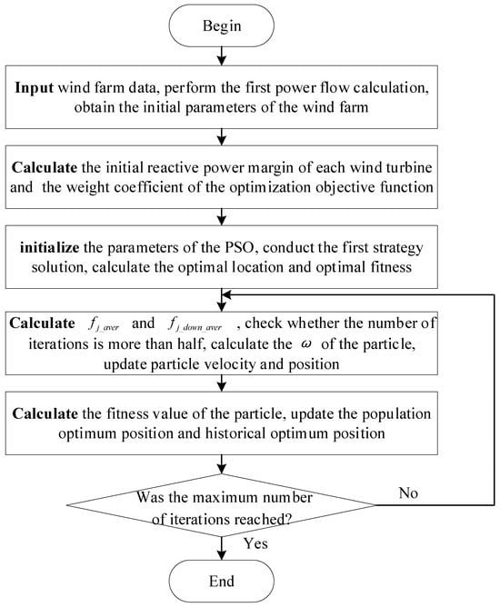
Figure 1.
UAPSO algorithm solution flowchart.
5. Case Analysis
5.1. Simulation Parameter Settings
The OWF structure used in this paper is shown in Figure 2. The installed capacity of the WF is 300 MW, with each WT having a rated power of 3 MW. There are 10 WTs connected on each feeder line, with a distance of 2 km between adjacent WTs. There are a total of 10 feeder lines. SVGs are connected to the primary side of the step-up transformer at node 3. The grid connection point (node 1) is set as the slack bus for the WF power flow calculation.
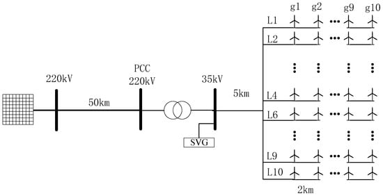
Figure 2.
OWF structure.
The distance from the offshore booster station to the swing bus is about 50 km. XLPE insulated submarine cables of 220 kV AC are used, and XLPE insulated submarine cables of 35 kV are used between the WTs (2 km) and between the WTs and the offshore booster station (5 km), with an operating temperature of 20 °C. The specific parameters are shown in Table 1.

Table 1.
Parameter list for submarine cables.
The basic parameters of the 3 MW permanent magnet synchronous WT are shown in Table 2.
Table 2.
Parameters of 3 MW permanent magnet synchronous wind generator.
5.2. Comparison of the Optimization Effects of Different Algorithms
To validate the effectiveness of the proposed improved particle swarm algorithm in this paper, the traditional PSO algorithm and dynamic weighting particle swarm algorithm (DPSO) are selected to compare the optimization results. Under the operating condition where the active power output of the WT is 2.8 MW and the reactive power output limit is 1 MW, the voltage reference value is set to 0.97 p.u. The optimization objective function is formulated using Equation (4). The optimization results of each algorithm are shown in Figure 3 and Figure 4.
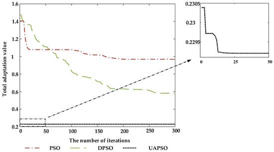
Figure 3.
Iteration curves for fitness values of different algorithms.
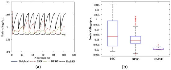
Figure 4.
Node voltage values after optimization by different algorithms: (a) node voltage graph and (b) nodal voltage box diagram(where red + corresponds to outliers).
Figure 3 and Figure 4 show the fitness iteration curves and WF node voltage curves for different algorithms. In Figure 3, it can be observed that the uniform adaptive algorithm converged to the vicinity of the optimal value within the first 50 iterations, while PSO and DPSO gradually converged to local optimal values after 250 iterations. In Figure 4a,b, it can be observed that compared with the DPSO algorithm and the PSO algorithm, the reactive power optimization strategy derived from the UAPSO algorithm can bring the voltages of each node closer to , effectively addressing the issue of excessive voltage deviation at the terminals of WTs at ends of the feeder line. This enables the terminal voltages of each wind turbine generator to accurately adhere to the specified voltage reference value. The comparative analysis reveals that the proposed uniform adaptive algorithm can effectively expand the search range of the particle swarm, avoiding local optima while achieving a fast convergence speed. It can rapidly determine the optimal strategy, yielding significantly better optimization results compared with PSO and DPSO.
Figure 5 shows the reactive power output of WTs obtained from the different algorithms’ optimization strategies. In the figure, it can be observed that the reactive power output of WTs in the optimization strategy obtained by UAPSO is more uniform. The difference in reactive power margin among WTs on the same feeder line is within 10%. However, there is significant variation in the reactive power output of WTs obtained by PSO and DPSO, with differences in the reactive power margin exceeding 100% on some feeder lines. Additionally, some WTs do not retain reactive power margins. In the event of a sudden drop or rise in busbar voltage, WTs may be unable to provide sufficient reactive power compensation, leading to the possibility of terminal voltages exceeding the safe and stable range.
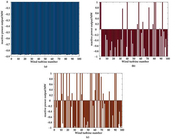
Figure 5.
Optimized reactive power output of WTs calculated using different algorithms: (a) UAPSO algorithm; (b) DPSO algorithm; (c) PSO algorithm.
The solution durations of the three optimization algorithms are shown in Table 3.
Table 3.
Comparison of the solving time of the different algorithms.
In Table 3, it can be seen that the solving time of the UAPSO algorithm is less than that of PSO and DPSO, with a speed improvement of about 10%. This is because the uniform initialization method expands the initial search range of the particle swarm, allowing particles to quickly search near the optimal solution. Meanwhile, the adaptive inertia coefficient method assigns a larger search speed to particles in the initial search stage, enabling particles to quickly search the solution space. In the later search stage, smaller search speeds are allocated to particles, enabling them to search in a small range near the optimal solution, thus improving the solution accuracy. In summary, the UAPSO algorithm not only enhances the search accuracy but also improves the search speed of the particle swarm.
5.3. Comparison of Optimization Results for Different Optimization Objectives
To demonstrate the significance of the optimization objective of the WT terminal voltage, different optimization objectives are set to compare the optimization effects. Optimization Objective 1 is the total optimization objective proposed in this paper; Optimization Objective 2 has the minimum deviation in grid-connected voltage and active power loss as the optimization objectives. The active power output of the wind turbine is set to 0.4 MW, and the is set to 0.96. The UAPSO algorithm is used for solving. The terminal voltage of the wind turbine generator after optimization is shown in Figure 6.
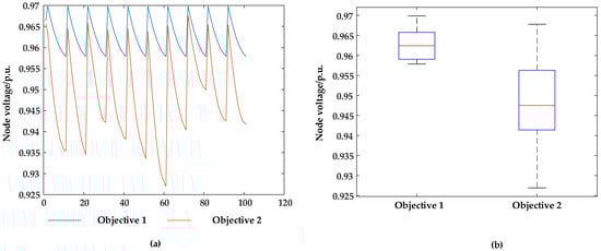
Figure 6.
Comparison of optimization results for different optimization objectives: (a) node voltage curve and (b) nodal voltage box line diagram.
In Figure 6, it can be observed that when the optimization objective does not include the deviation in the WT terminal voltage, although the grid-connected voltage can accurately approach the reference voltage, the WT terminal voltage decreases to below 0.95 p.u., and some WT terminal voltages even decrease to 0.928 p.u., severely affecting the safe and stable operation of the WT. However, when the deviation in the WT terminal voltage is included as an optimization objective, both the grid-connected voltage and the WT terminal voltage can accurately approach the reference voltage, ensuring that the WT terminal voltage remains stable within a safe range. Therefore, when optimizing the reactive power of offshore wind farms, it is also necessary to pay special attention to the problem that the WT terminal voltage easily exceeds limits.
5.4. Comparison of Optimization Effects of Different Multi-Objective Weighting Methods
To verify the effectiveness of optimizing the objective function with adaptive weighting coefficients, different combinations of weights for the objective function are selected to compare the optimization results. Under the operating condition where the active power output of the WT is 2.8 MW and the reactive power output limit is 1 MW, the voltage reference value is set to 0.97 p.u. The UAPSO algorithm is used for strategy optimization. The optimization results for each weight combination are shown in Figure 7 and Table 4.
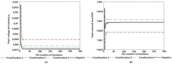
Figure 7.
Comparison of the optimization effect of different weight combinations when Uref = 0.97: (a) network loss and (b) voltage deviation.
Table 4.
Comparison of reactive power margins for different weighting combinations.
When the voltage reference value approaches the stable voltage boundary (0.95–1.05 p.u.) and the reactive power limit of WTs is relatively small, the calculated adaptive weighting coefficients correspondingly assign larger weights to voltage deviation and the reactive power margin. The resulting reactive power optimization strategy focuses on optimizing node voltage deviation and the reactive power margin. In Figure 7 and Table 4, it can be seen that the reactive power optimization strategy obtained by solving the adaptive weighting objective function sacrifices some of the grid loss optimization effects. However, it minimizes the voltage deviation and retains a larger reactive power margin. Reactive power strategies based on fixed weights cannot simultaneously optimize voltage and the reactive power margin effectively. Under harsher operating conditions in the WF, this may lead to terminal voltages of WTs exceeding safety limits or an insufficient reactive power margin, failing to meet requirements.
5.5. Adaptability of Adaptive Reactive Power Optimization Strategies under Various Operating Conditions
5.5.1. Optimization Effect of Different Active Outputs of WT
To validate the effectiveness of the adaptive weighting coefficients optimization objective and the UAPSO algorithm under different operating conditions in OWFs, the optimization results are compared across different conditions. In this case, the voltage reference value is set to 0.97 p.u. A comparison of the optimization results after optimization is shown in Figure 8 and Figure 9 and Table 5.

Figure 8.
Optimization of voltage under different operating conditions: (a) iterative curves of total voltage deviation and (b) the WT terminal voltage box line diagram(where red + corresponds to outliers).
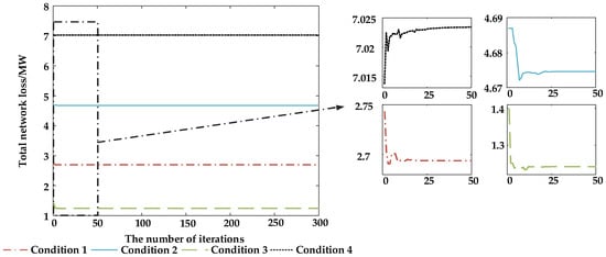
Figure 9.
Optimization of network losses under different operating conditions.
Table 5.
Reactive power margin for different operating conditions.
Figure 8 and Figure 9, respectively, compare the voltage and grid loss optimization effects under different operating conditions. In the figures, it can be observed that the optimized grid loss in the OWF is positively correlated with the active power output of the WTs. When the active power output is small, the optimized grid loss is also small; however, when the active power output is large, the optimized grid loss increases. At the same time, it can be seen that under different operating conditions, the total voltage deviation in the nodes in the WF is less than 1, indicating that the average deviation between the node voltages and the voltage reference value is less than 0.01 p.u. (a total of 103 nodes), and the optimized node voltages meet the requirements.
Table 5 compares the optimization effects of the reactive power margin of a single WT under different operating conditions. In the table, it can be observed that the weighting coefficients of the adaptive optimization objective function change with the real-time operating conditions. When the reactive power limit of the WT is small, the weighting coefficient corresponding to the reactive power margin is set to a large value to ensure that the WT retains a sufficient reactive power margin. When the reactive power limit of the WT is large, the weighting coefficient corresponding to the reactive power margin needs to be set to a small value. While ensuring that the reactive power margin of the WT meets the requirements, the focus is on reducing voltage deviation and grid loss, thereby improving the stability and economy of the WF operation.
From the above analysis, it can be seen that the adaptive reactive power optimization strategy based on the UAPSO algorithm can achieve good optimization results under various operating conditions.
5.5.2. Optimization Effect of Different Voltage References
To verify the effectiveness under different voltage reference values, different voltage reference values are selected to compare the optimization results. Simulations are conducted under the condition that the WT has an active power output of 2.8 MW and a reactive power output limit of 1 MW. The comparison of optimization results after optimization is shown in Figure 10 and Table 4.
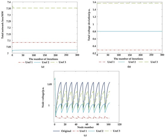
Figure 10.
Comparison of optimization effects with different voltage references: (a) network loss; (b) voltage deviation; and (c) node voltage.
Figure 10 presents a comparison of voltage and network loss optimization effects under different voltage reference values. In Figure 10a, it can be observed that the network loss after optimization in OWFs is positively correlated with the active power output of WTs. When the active power output is small, the optimized network loss is small, and when the active power output is large, the optimized network loss is large. In Figure 10b, it can be seen that under different voltage reference values, the optimized voltage values of each node can closely match the reference values. The voltage deviation between WTs at both ends of the same feeder line is less than 0.03 p.u. In Figure 10c, it can be observed that under different operating conditions, the total voltage deviation in the nodes in the WF is less than 1, indicating that the average deviation between each node voltage and the voltage reference value is less than 0.01 p.u. (across 103 nodes), and the optimized node voltages meet the requirements.
Table 6 compares the optimization effects of reactive power reserves for a single WT under different voltage reference values. In the table, it can be seen that the weighting coefficients corresponding to voltage deviation change with the voltage reference value. When the difference between node voltage and the voltage reference value is small, the weighting coefficients corresponding to voltage deviation are set to small values, emphasizing the reduction in network loss and an improvement in reactive power reserves of WTs while ensuring that the voltage deviation meets the requirements, thereby enhancing the economic efficiency and robustness of WF operation. When the difference between node voltage and the voltage reference value is large, the weighting coefficients corresponding to voltage deviation are set to large values, effectively reducing the voltage deviation and ensuring that each node voltage is within a safe and stable range, thereby enhancing the stability of WF operation.
Table 6.
Reactive power margins at different voltage references.
From the above analysis, it can be seen that the adaptive reactive power optimization strategy based on the UAPSO algorithm achieves good optimization effects under different voltage reference values.
6. Conclusions
This paper investigates the reactive power optimization problem in OWFs, considering multiple sub-objectives including voltage control, active power loss, and reactive power reserve. Because of the varying importance of different sub-objectives under different operating conditions, fixed weighting coefficients cannot accurately represent the dynamic changes in the importance of different sub-objectives. Therefore, innovatively, the weighting coefficients of each sub-objective in this paper are adaptively adjusted according to real-time operating conditions. Meanwhile, to address the issue of an insufficient search range and susceptibility to local optimal values in PSO algorithms, improvements are made based on uniform initialization and adaptive inertia coefficients. The research results demonstrate the following:
- 1.
- The proposed method can reduce the voltage deviation and active power loss in OWFs, increase the reactive power reserve, and enhance the stability, economy, and robustness of WF operation.
- 2.
- The uniform initialization of particles in PSO broadens the search range, avoiding getting stuck in local optimal values, and adaptive inertia coefficients effectively accelerate the convergence speed of the particle swarm.
- 3.
- When the operating state of the WF changes, the weighting coefficients between optimization objectives can be adaptively adjusted based on real-time operating conditions, ensuring that important objectives under different conditions are prioritized and guaranteed.
Author Contributions
Conceptualization, C.F. and J.L.; methodology, C.F.; software, C.F.; validation, C.F., J.L., J.Z. and M.M.; formal analysis, C.F.; investigation, C.F.; resources, J.L.; data curation, C.F.; writing—original draft preparation, C.F.; writing—review and editing, J.L.; visualization, C.F. and M.M.; supervision, C.F.; project administration, J.Z. and M.M.; funding acquisition, J.Z. and M.M. All authors have read and agreed to the published version of the manuscript.
Funding
This work was supported in part by the National Natural Science Foundation of China under Grant 62173148 and Grant 52377186, in part by the Natural Science Foundation of Guangdong Province under Grant 2022A1515010150 and Grant 2023A1515010184, in part by the Basic and Applied Basic Research Foundation of Guangdong Province under Grant 2022A1515240026, in part by the Technology Project of Southern Power Grid Co., Ltd. under 030800KC23040003, and in part by the Joint Laboratory of Energy Saving and Intelligent Maintenance for Modern Transportations.
Data Availability Statement
The data presented in this study are available in this article.
Conflicts of Interest
Author Ming Ma was employed by the company Electric Power Scientific Research Institute of Guangdong Power Grid Co., Ltd. The remaining authors declare that the research was conducted in the absence of any commercial or financial relationships that could be construed as a potential conflict of interest.
References
- Yan, P.Q.; Wang, Z.P.; Chen, Z.X.R. Reactive power optimization for wind farm considering impact of topology. Power Syst. Prot. Control 2016, 44, 76–82. [Google Scholar]
- Fu, Y.; Pan, X.L.; Huang, L.L. Reactive power optimization for offshore wind farm considering reactive power regulation capability of doubly-fed induction generators. Power Syst. Technol. 2014, 38, 2168–2173. [Google Scholar]
- Zhang, L.; Jiang, Z.Q.; Ni, J.H.; Zhou, H.; Lu, Y.U.; Xiang, J. Internal reactive power optimization of offshore wind farms using second-order cone convex relaxation. Electr. Power Constr. 2024, 1, 92–101. [Google Scholar]
- Wang, Y.; Wang, T.; Zhou, K.P.; Cao, K.; Cai, D.F.; Liu, H.G.; Zhou, C. Reactive power optimization of wind farm considering reactive power regulation capacity of wind generators. In Proceedings of the IEEE PES Innovative Smart Grid Technologies Asia, Chengdu, China, 21–24 May 2019. [Google Scholar]
- Ma, M.; Du, W.L.; Tao, R.; Wang, M.; Liao, K. Hierarchical Voltage Optimal Control Strategy of Wind Farms Based on Robust Optimization. J. Tianjin Univ. (Sci. Technol.) 2021, 54, 1309–1316. [Google Scholar]
- Wu, X.; Liu, T.Y.; Jiang, X.C.; Sheng, G.H. Research on reactive power optimization of offshore wind farm based on improved genetic algorithm. Electr. Meas. Instrum. 2020, 57, 108–113. [Google Scholar]
- Xing, Z.; Yan, N.; Xiao, W.Q.; Li, W. Multi-timescale multi-objective reactive power optimization of dispersed wind farm. Electr. Mach. Control 2016, 20, 46–52. [Google Scholar]
- Niu, T.; Guo, Q.L.; Sun, H.B.; Liu, H.T.; Zhang, B.M.; Du, Y.L. Dynamic reactive power reserve optimization in wind power integration areas. IET Gener. Transm. Distrib. 2018, 12, 507–517. [Google Scholar] [CrossRef]
- Ma, H.; Ma, L.L.; Zhang, Z.X.; Zhu, Y.Z.; Li, G.H.; Wang, Y.Q. Optimal reactive power allocation of a wind farm with SVG for voltage stability enhancement. In Proceedings of the International Conference on Power System Technology, Jinan, China, 21–22 September 2023. [Google Scholar]
- Ni, F.Y.; Qin, X.H.; Huang, Z.H.; Yang, Y.X.; Niu, Z.B.; Zuo, W.L. Optimal control strategy of reactive power and voltage for wind farm based on LinWPSO algorithm. In Proceedings of the Asia Conference on Energy and Electrical Engineering, Chengdu, China, 21–23 July 2023. [Google Scholar]
- Xiao, Y.Q.; Wang, Y.; Sun, Y.P. Reactive power optimal control of a wind farm for minimizing collector system losses. Energies 2018, 11, 3177. [Google Scholar] [CrossRef]
- Wang, D.S.; Tan, D.P.; Liu, L. Particle swarm optimization algorithm: An overview. Soft Comput. 2017, 22, 387–408. [Google Scholar] [CrossRef]
- Zishan, F.; Akbari, E.; Montoya, O.D.; Giral-Ramírez, D.A.; Molina-Cabrera, A. Efficient PID control design for frequency regulation in an independent microgrid based on the hybrid PSO-GSA algorithm. Electronics 2022, 11, 3886. [Google Scholar] [CrossRef]
- Kandati, D.R.; Gadekallu, T.R. Federated learning approach for early detection of chest lesion caused by COVID-19 infection using particle swarm optimization. Electronics 2023, 12, 710. [Google Scholar] [CrossRef]
- Xu, Q.H.; Lan, Y. Reactive power optimization of distribution network with distributed power based on MOPSO algorithm. In Proceedings of the International Conference on Clean Energy and Power Generation Technology, Zhenjiang, China, 9–11 December 2022. [Google Scholar]
- Li, J.H.; Huang, H.Y.; Lou, B.L.; Peng, Y.; Huang, Q.X.; Xia, K. Wind farm reactive power and voltage control strategy based on adaptive discrete binary particle swarm optimization algorithm. In Proceedings of the Asia Power and Energy Engineering Conference, Chengdu, China, 29–31 March 2019. [Google Scholar]
- Singh, N.; Sharma, A.K.; Tiwari, M.; Jasinski, M.; Leonowicz, Z.; Rusek, S.; Gono, R. Robust control of SEDCM by Fuzzy-PSO. Electronics 2023, 12, 335. [Google Scholar] [CrossRef]
- Song, Y.J.; Liu, Y.; Chen, H.Y.; Deng, W. A multi-strategy adaptive particle swarm optimization algorithm for solving optimization problem. Electronics 2023, 12, 491. [Google Scholar] [CrossRef]
- Hsieh, F.S. Comparison of a hybrid firefly–Particle swarm optimization algorithm with six hybrid firefly–Differential evolution algorithms and an effective cost-saving allocation method for ridesharing recommendation systems. Electronics 2024, 13, 324. [Google Scholar] [CrossRef]
- Jiang, F.; Li, T.; Cui, D.; Zhang, C.L.; Xiao, H.F. Reactive power optimization strategy of wind farm based on particle swarm optimization algorithm. In Proceedings of the 2022 IEEE Transportation Electrification Conference and Expo, Asia-Pacific, Haining, China, 28–31 October 2022. [Google Scholar]
Disclaimer/Publisher’s Note: The statements, opinions and data contained in all publications are solely those of the individual author(s) and contributor(s) and not of MDPI and/or the editor(s). MDPI and/or the editor(s) disclaim responsibility for any injury to people or property resulting from any ideas, methods, instructions or products referred to in the content. |
© 2024 by the authors. Licensee MDPI, Basel, Switzerland. This article is an open access article distributed under the terms and conditions of the Creative Commons Attribution (CC BY) license (https://creativecommons.org/licenses/by/4.0/).