Applications of the TL-Based Fault Diagnostic System for the Capacitor in Hybrid Aircraft

Abstract

The article concerns the problem of capacitor diagnosis in a hybrid aircraft. Capacitors are one of the most commonly damaged components of electrical vehicle drive systems. The result of these failures is an increase in voltage ripple. Most known analytical methods are based on frequency spectrum analysis, which is time-consuming and computationally complex. The use of deep neural networks (DNNs) allows for the direct use of the measurement signal, which reduces the operating time of the overall diagnostic system. However, the problem with these networks is the long training process. Therefore, this article uses transfer learning (TL), which allows for the secondary use of previously learnt DNNs. To collect data to learn the network, a test bench with the ability to simulate a capacitor failure was constructed, and a model based on it was made in the MATLAB/Simulink environment. A convolutional neural network (CNN) structure was developed and trained by the TL method to estimate the capacitance of the capacitor based on signals from the Simulink-designed model. The proposed fault diagnostic method is characterised by a nearly 100% efficiency in determining capacitance, with an operating time of about 10 ms, regardless of load and supply voltage.

1. Introduction

According to the Strategic Plan for Research and Development of the Clean Aviation programme, technologies in the aviation industry are to be developed by 2035 to create an aircraft with a reduction of at least 30% in greenhouse gas emissions compared to the state of the art in 2020 [1]. One of the elements identified in the programme is a power distribution system for hybrid regional aircrafts [2,3]. In this type of system, there are numerous energy converter systems, of which the components that are most often damaged are intermediate circuit capacitors [4,5]. Significantly crucial capacitors in hybrid aeroplanes are located in the DC link of the power converter connected to the electrical drive, as these minimise DC voltage ripple. In this paper, only rectifier and DC links of propulsion system are taken into consideration, as these are sufficient to verify the proposed methods.

The decrease in capacitance of a capacitor indicates its progressive degradation. Depending on the type of capacitor, the end-of-life criterion is a different percentage of capacitance drop [6]. The effect of the degradation process is an increase in the ripple of the DC link voltage. In the literature, there is an observable increase in interest in diagnostic systems for these components of power conversion systems. In the article [7], MPPF-type capacitors (metallized polypropylene film) were proposed for aerospace applications, which, unlike electrolytic capacitors, which are often described within the diagnostics framework [8,9,10,11,12,13,14,15], do not have ESR (Equivalent Series Resistance) changes large enough to allow determination of the degree of degradation. For the above reasons, this article focusses on determining the change in capacitance of capacitors in the intermediate circuit to develop a universal method.

It should be noted that capacitance diagnosis of a capacitor can be performed both offline [8,9] and online [10,11,12,13]. To avoid the need to interfere with the topology of the power electronics system and to minimise the impact on the control algorithm, we focus on diagnostics in the operating state. However, it is still necessary to process the measured signal through a filter to improve the accuracy of estimating the capacitance of a capacitor in a circuit [7]. Another approach is the method described in [10], which uses only one signal (voltage in the intermediate circuit). Unfortunately, accurate knowledge of the value of the inductance included in the intermediate circuit is required, which can change during use. The authors in [11,16] propose using a Kalman filter to estimate both the capacitance and ESR of a capacitor. This solution is problematic due to the high computational complexity involved in performing matrix operations. Another example of a computationally complex method is [12,17], where the least squares method was used to estimate the capacitor parameters. In the case of [13], the determination of capacitance is made using the short-time Fourier transform (STFT). Although this type of frequency analysis provides estimation in a short time, it requires measurements of both the voltage and current of the capacitor. The same is true in [18], where the capacitance is determined as the quotient of the integral of the current and voltage ripple.

The limitations mentioned above indicate the need to develop a method that does not require signal preprocessing or knowledge of additional circuit parameters beyond the initial capacitance. In addition, it is not computationally complex and uses as few sensors as possible.

For a long time now, the increasing influence of artificial-intelligence-based solutions in diagnostics [19,20,21] has been observed. This is due, among other things, to the desire to reduce the response time in the fault detection process and to fully automate the diagnostic process. Initially, neural network systems were based on signal analysis methods [22], where expert knowledge was replaced by the ability to approximate shallow structures based on specific diagnostic symptoms. However, the problem of classical shallow networks such as multilayer perceptrons, Kohonen classifiers, or networks with radial activation functions is the need to preprocess the diagnostic signal to extract damage features from it. Therefore, it was necessary to find a solution that would allow direct use of the diagnostic signal. One of the most widely used approaches to direct processing in recent years is the use of deep neural networks (DNNs) [23,24,25]. Construction of DNNs is based on the use of many different layers of neurones, each of which processes the data provided to it from the previous layer, creating new higher-order features from basic features [23,26]. Thus, DNNs can also be used for pre-processed signals [27], but their significant advantage is that they can work directly with the diagnostic signal [28,29].

The problem with using DNNs is the need for large datasets and long learning times due to the extensive architecture of deep networks. In addition, the selection of hyperparameters for these networks is not defined by formal rules, which further complicates their implementation. It is worth noting that, both in the case of shallow and deep structures, changing the object or extending the tasks posed to the diagnostic systems requires retraining and selection of the network structure. Given this, it is important to ensure the universality of diagnostic symptoms while maintaining their automatic. This issue is currently being implemented through the use of deep neural networks, taught by the idea of transfer learning (TL) [30,31]. The popularity of this technique is based on the use of previously learnt features and the appropriate combination of their participation in a new dataset that represents a new diagnostic problem. In addition to significantly reducing the implementation time of DNN-exploiting systems, this method ensures the full use of the information from the Simulink-designed model of the object. This article presents the application of the idea of deep convolutional network TL in the system of detection and classification of capacitor faults using information from a simplified Simulink-designed model. It is worth noting the practicality of the proposed network, which, compared to well-known and used convolutional networks, such as VGG-16 [32], VGG-19 [33], and AlexNet [34], which have 138 million, 144 million, or 60 million parameters, respectively, has a much smaller number of parameters (44,000), occupying only 96.5 kB of memory. Moreover, this system makes use of information from the model in the diagnostic system and performs the verification of the system on the real object. This approach ensures a full use of the model, as well as a complete understanding of the initial stage of damage without physically damaging the test object.

2. Capacitor Fault Detection System Using Transfer Learning—Data Development

In addition to an expanded number of neural connections, deep neural networks require an extensive dataset used in the learning process. This process is based primarily on stochastic methods that use randomly selected learning data packages to average gradient values. Therefore, it is important to develop an appropriate number of learning data for different operating states of the object, taking into account the possible even distribution of learning examples into recognised categories. In the study, two sets of learning data were used. The first was the results of simulation studies conducted for a simplified object model. This package was used to develop universal symptoms to recognise damage during operation on the real object. The second set was developed from measurements using a specially prepared physical model of the object under study. These data were used in the second stage of adaptation of the weighting coefficients for the idea of TL described in Section 3. Measurements made on the physical model provided a reference point during experimental verification of the proposed diagnostic system.

2.1. Physical and Simulink-Designed Model of the Experimental Bench

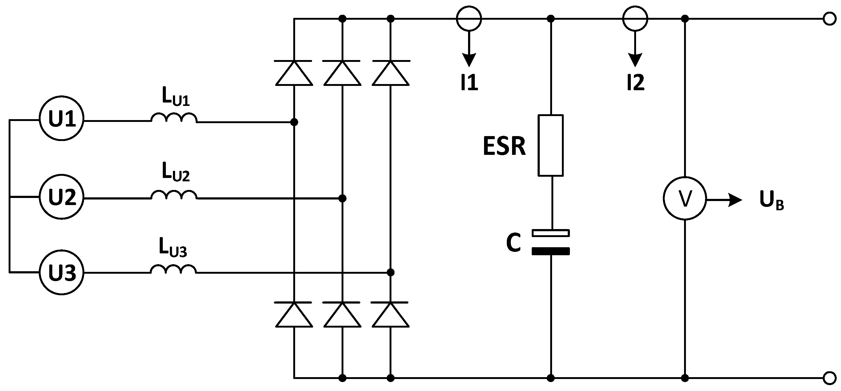
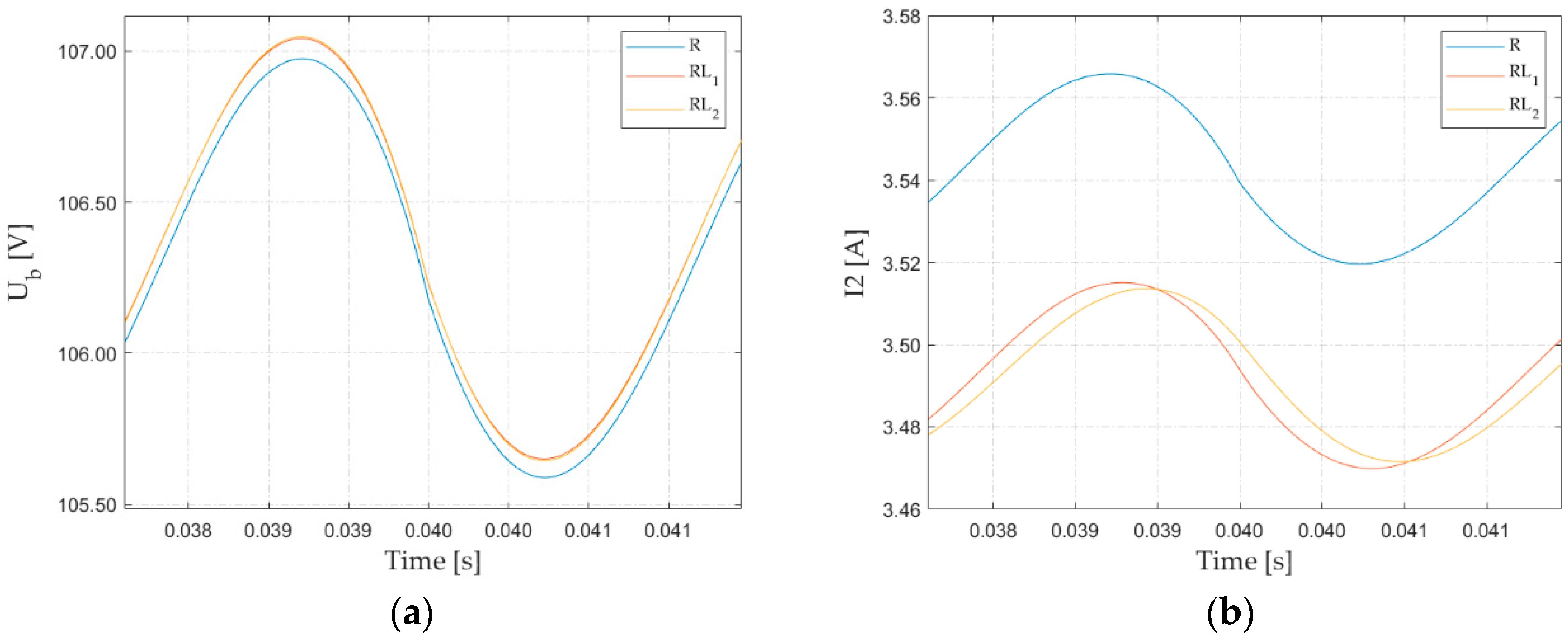
The voltage converter is designed to test the influence of changing capacitance of capacitors in a DC circuit on the shape of current and voltage waveforms. The converter design uses a three-phase rectifier bridge with a rated current of 35 A and a maximum operating voltage of 1000 V. The DC link circuit uses a bank of five capacitors with a capacitance of 470 µF each and an operating voltage of 400 V. Capacitors can be connected to the DC circuit by means of special jumper keys, which ensure flexible configuration of the connection topology. Thanks to applied design, it is possible to obtain series, parallel, or mixed connections of capacitors, resulting in a change in the overall capacitance of the system. Figure 1 represents the schematic diagram of the converter.

The converter is equipped with a current measurement system, I1 on the input side and I2 on the output side. The measurement system uses hall effect transducers of the LEM LH 25-NP type, which are configured to measure currents in the range −8 … +8 A. Figure 2 shows the connection diagram of the current measurement system and the power supply system.

Additionally, the entire device has the ability to measure the voltage of the DC circuit (UB). Figure 3 represents a schematic diagram of the voltage measurement system. This system is equipped with an insulated hall effect voltage sensor of the LEM LV 25-P type with resistors that limit the input current. With this configuration, the system can measure voltages in the range of 10 …400 V.

Real capacitors can be represented by a series circuit consisting of capacitance, resistance, and inductance components (Figure 4). However, due to the inductance component of the capacitor being mostly pronounced for the high frequency signals (Figure 5) and low-frequency nature of the conducted experiment, the inductance (ESL—Equivalent Series Inductance) can be omitted in the model.

Based on the converter topology (Figure 1), a Simulink-designed model was made in the Simulink environment (Figure 6). Such a model allows for a more precise change of DC-link capacitance. In addition, a wide range of loads can be applied to this model. The purpose of the model is to generate data, based on capacitance measurements and theoretical data of other parameters, to provide it for neural network training. Moreover, by combining measured and calculated parameters, the noise input to the constructed voltage converter can be identified. It is worth mentioning that the model is made using the Simscape Electrical toolbox from Simulink. This toolbox provides a wide range of ready-made blocks that are based on mathematical descriptions of components used in the field of electrical engineering [35].

This real capacitor model allows for the representation of its voltage u and current i relationship using the capacitance of capacitor C and the ESR (1). Furthermore, the impedance Z module can be described by (2) in the pulsation ω domain. Combining the mathematical descriptions of the DC link capacitors (1–2) and the impedance module values based on mean voltage U and mean current I measurements (3) proves that the analysis of these two signals is sufficient for capacitance assessment:

$$i=C·\frac{du}{dt}+\frac{1}{ESR}·u$$

(1)

$$\left|Z\right|=\sqrt{{ESR}^2+{\left(\frac{1}{\omega ·C}\right)}^2}$$

(2)

$$\left|Z\right|=\frac{\left|U\right|}{\left|I\right|}$$

(3)

where: i—current, u—voltage, I—mean current, U—mean voltage, C—capacitance, ESR—Equivalent Series Resistance, Z—impedance, ω—electrical pulsation, t—time.

The DC link parameters are presented as singular capacitance and ESR components. Other changeable parameters are line inductances and voltages, as the converter was powered from an autotransformer with line-to-line voltage regulation (voltage change also affects winding inductance).

The designed model allows us to simulate the degradation process of the capacitor under different load and power supply configurations. This range of possible changes in the model can represent the internal and external factors that affect the electrical parameters of the system.

The impact of the load configuration can be seen in Figure 7. Three types of load were simulated:

• R (R = 30.45 Ω);
• RL₁ (R = 30.45 Ω, L = 2.5 mH);
• RL₂ (R = 30.45 Ω, L = 7.5 mH).

The additional load inductance causes a voltage increase and a current decrease. Moreover, different inductance values affect the phase shift of electrical signals. As can be seen, the load parameters affect the measurement data. Therefore, testing for different types of loads is crucial for a proper assessment of the diagnosis method.

The Simulink-designed model sensitivity test was carried out regarding the change in the root mean square values of the voltage sources U1, U2, and U3 (RMS) (Figure 8). The test input values were as follows:

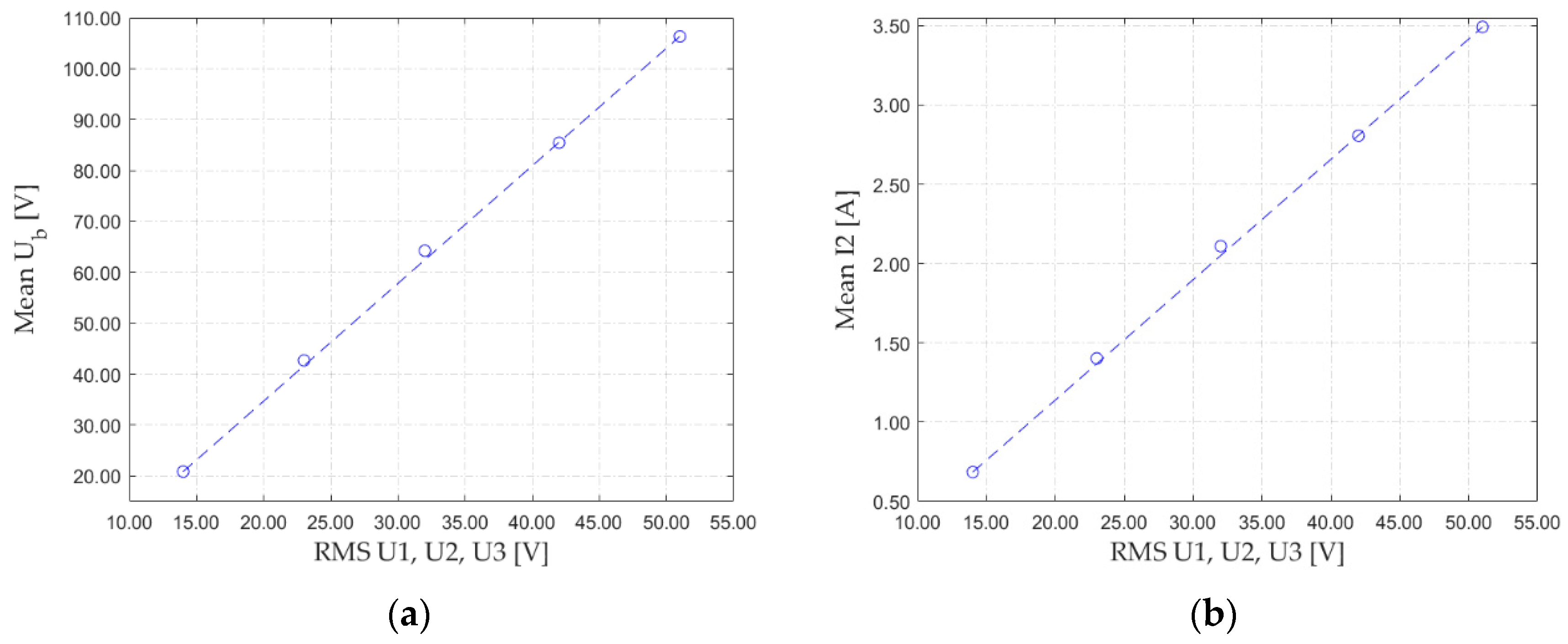
• U1 = U2 = U3 = 14 V;
• U1 = U2 = U3 = 23 V;
• U1 = U2 = U3 = 32 V;
• U1 = U2 = U3 = 42 V;
• U1 = U2 = U3 = 51 V.

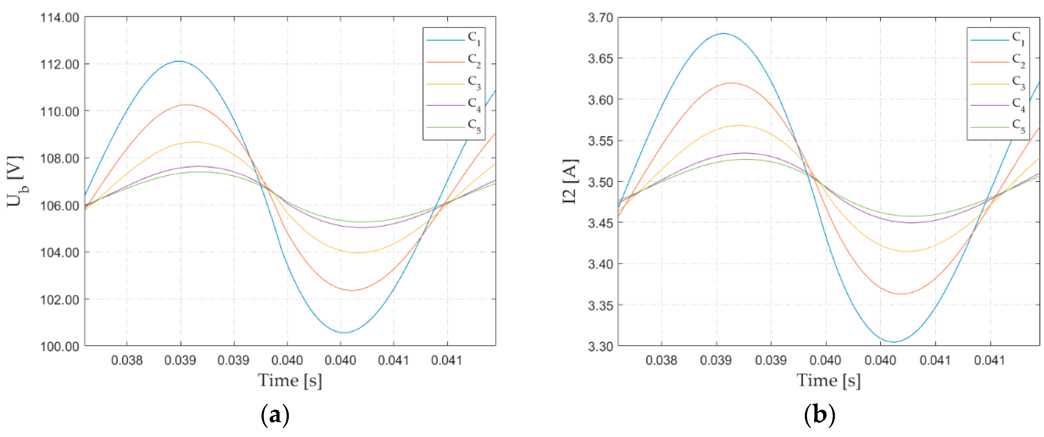
As can be seen in Figure 8, the higher the voltage source RMS values, the higher the mean voltage Ub on the DC link that can be observed. However, the mean load-side current I2 also increases the voltage increase.

The influence of the DC link capacitance value was also analysed (Figure 9). During the simulations, the following capacitance values were taken into account:

• C₁ = 103.3 μF;
• C₂ = 137.4 μF;
• C₃ = 207.3 μF;
• C₄ = 346.2 μF;
• C₅ = 414.3 μF.

In Figure 9, it can be observed that the higher the capacitance, the smaller the DC link voltage and the ripple amplitudes of the load current.

The results of the Simulink-designed model sensitivity analysis that can be seen in Figure 7, Figure 8 and Figure 9 prove that model behaviour changes due to parameters of load, power supply, and DC link. A comparative analysis of the results of simulation tests and measurements on the physical model was carried out to verify the correctness of the model in the next stage of the study.

2.2. Validation of the Simulink-Designed Model

The model was validated by comparing two of its output signals, the U_B voltage (Figure 10a) and the I2 current (Figure 10b) with measurements taken from the constructed system. The same capacitance and ESR as were used during the measurements were applied to the Matlab Simulink model.

The DC-link parameters were obtained using an LCR meter. The entire system was powered by an autotransformer. For data capture, a measuring station consisting of dSpace 1103 was used. The probed signal was sampled at a rate of 10 kHz and saved for further mathematical analysis. Regarding the model, each of the power supply phases, despite being asymmetric, had an RMS voltage value of around 50 V. In the validation process, the topology used consisted of the singular capacitor (C = 414.3 µF; ESR = 0.27 Ω) with load RL (R = 30.45 Ω, L = 7.5 mH). The simulation step of 1e-7 s was chosen to include every modelled phenomenon. In both cases (Figure 10), simulation output and the measured signals are similar (three-phase power supply voltage imbalance that affects rectified voltage and current). Phase and ripple differences are caused by difficulties in conducting inductance measurements of autotransformer secondary windings. Additionally, the experimental station is supplied by a power grid that can be affected by voltage and phase-shift unbalance. These disturbances are subject to the supply and demand of the power grid and can fluctuate unpredictably, providing another source of simulation–experiment discrepancies. Taking into account nature (Figure 10) and small differences in the RMS, maximal, minimal, and ripple values of the analysed signals (

Table 1. Model validation signals’ parameters.

Parmeter		Signal
		I2 [A]	UB [V]
RMS	Measurements	3.8022	116.0127
	Simulations	3.7854	115.2754
	Error [%]	0.4424	0.6356
Max	Measurements	3.9665	121.0847
	Simulations	3.9658	120.9746
	Error [%]	0.2435	0.0909
Min	Measurements	3.6467	111.2482
	Simulations	3.6162	109.5845
	Error [%]	0.8341	1.4955
Ripple	Measurements	0.3198	9.8365
	Simulations	0.3406	11.3901
	Error [%]	6.4898	15.7944

), the simulated model correctly represents the voltage converter system and can be used to perform TL.

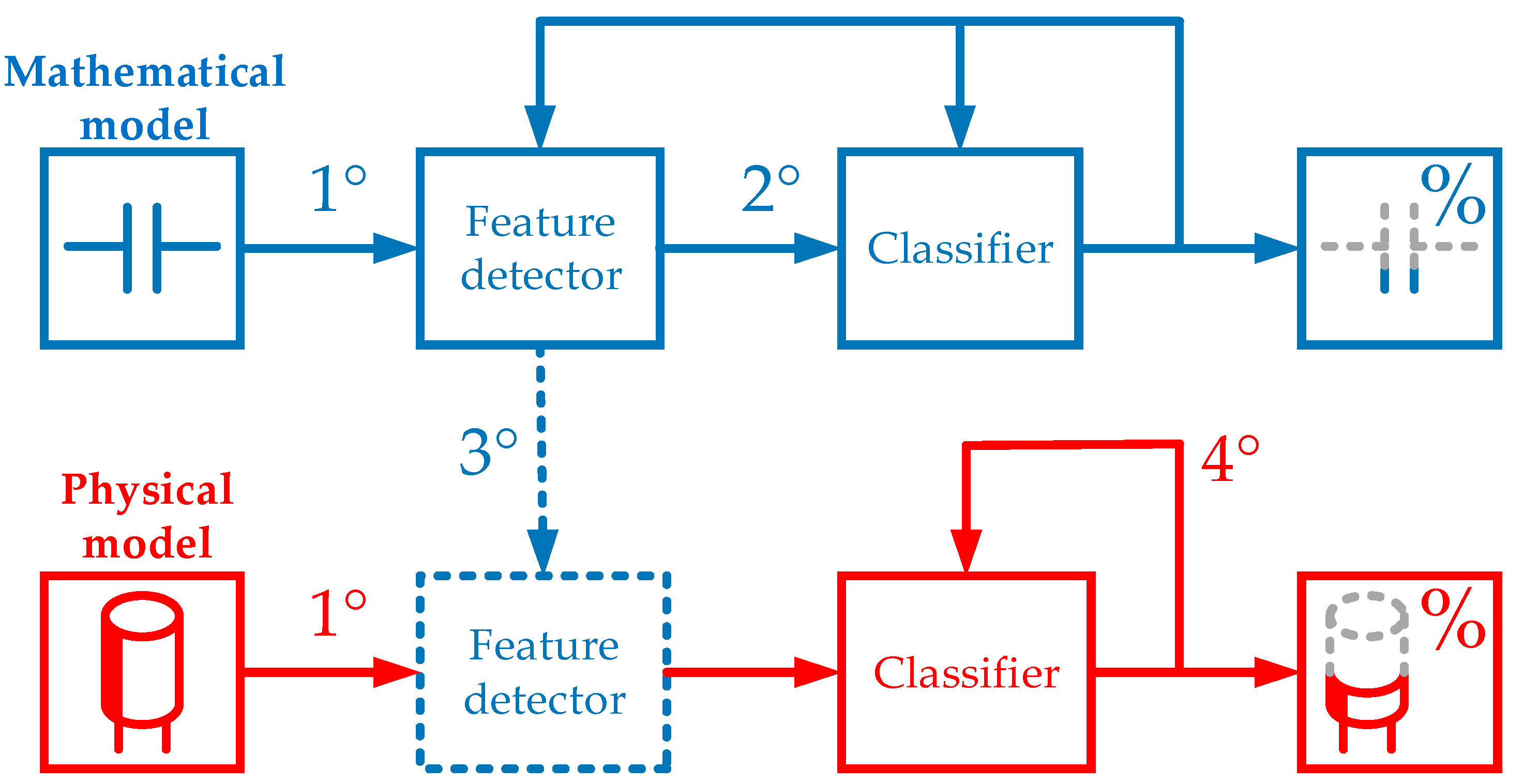
3. Convolutional Neural Network-Based Diagnostic System Using Transfer Learning

3.1. Idea of Transfer Learning

The implementation of the deep convolutional network TL technique for the proposed diagnostic task is carried out in two stages. In the first stage, the process of training the underlying structure (the blue part of Figure 11 below) is carried out on the basis of the data developed for information from the Simulink-designed model of the object. The input vector, containing 100 samples of the current and output voltage signals, was transformed into a matrix of 10 × 10 × 2 dimensions. It should be noted that the classical approach to convolutional networks describes the network as made up of contained layers that involve the extraction of features of the input matrix (convolutional layers) and the assignment of recognised features to one of the considered categories (classifier). Consequently, the first process to adapt the weighting factors of the underlying structure involves updating the parameters of the feature detector and the classifier. The verification of this step is carried out on the basis of the evaluation of the network response and the modelled capacitance percentage of the capacitor (capacitor failure stage).

The second stage involves using the information retained in the weight coefficients of the feature detector (convolutional layers) in a new structure operating on the real object. Feature transfer involves blocking the adaptation process of the weight coefficients of the convolutional layers and performing the learning process of the classifier only. In this way, the structure does not acquire the ability to recognise features (it uses symptoms trained on the model) and only determines how to combine known features to solve the problem for the real object. In this stage, the input data come from the physical model—the response of the network is the percentage of the capacitance of the capacitor (λ) from the model, while only the parameters of the multilayer perceptron (classifier) are adapted. The parameters of the structures of the convolutional neural networks summarised in

Table 2. Parameters of the CNN structure used in the study.

Convolutional Neural Network Structure		Number of Learnable
		Classic Training	Transfer Learning
Feature detector	Convolutional layer: 30 filters, 3 × 3	380	0
	Normalisation Layer	40	0
	Pooling Layer: max, 3 × 3, stride 2 × 2	0	0
	Convolutional layer: 40 filters, 3 × 3	7240	0
	Normalisation Layer	80	0
	Pooling Layer: max, 3 × 3, stride 2 × 2	0	0
	Convolutional layer: 60 filters, 3 × 3	21,660	0
	Normalisation Layer	120	0
	Pooling Layer: max, 3 × 3, stride 2 × 2	0	0
Classifier	Fully Connected Layer: 60 neurones	14,460	14,460
	Fully Connected Layer: 8 neurones	488	488
Total		44,468	14,948

clearly show the advantage of the TL method over the classical training process. This fact is due to the blocking of the weighting coefficients of the feature detector layers, making the number of parameters required for tuning much smaller. As a result, the weight adaptation process can be much faster and is computationally no different from the classical multilayer perceptron training process.

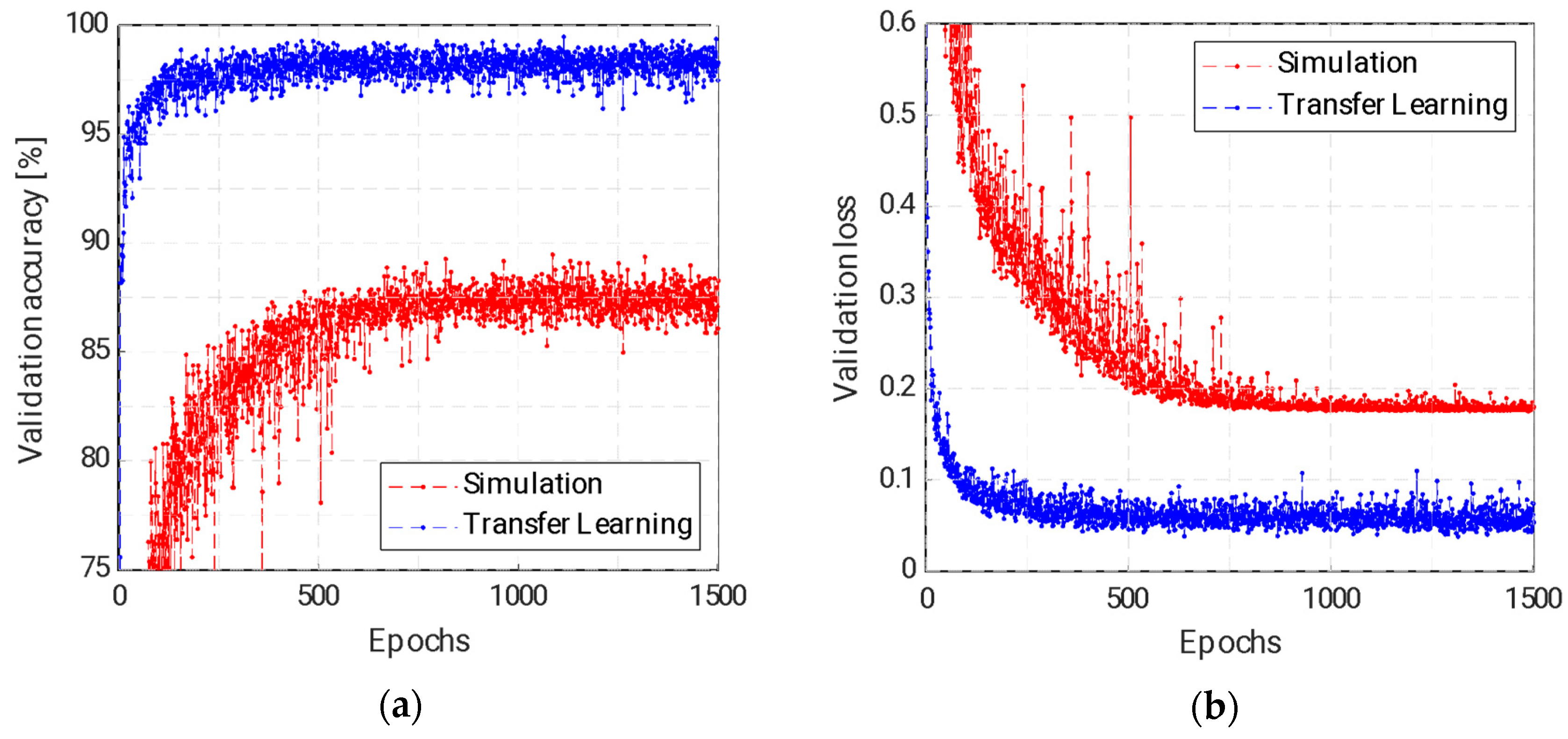
3.2. Convolutional Network Training Process According to Transfer Learning

Based on the training data developed, the process of adapting the weighting coefficients of the convolutional network was carried out according to the stochastic gradient descent algorithm with momentum. The learning process included 2000 epochs with an initial learning factor of 0.002 and a momentum factor of 0.9. The training process was based on the use of mini-data packages containing 32 randomly selected samples from the learning dataset. To present the network with all examples, each learning epoch consisted of 31 iterations, during which the precision of the neural network was verified. The learning dataset contained 125 examples for each recognised class of damage (a total of 1000 cases). The input matrices of the network developed from the model were determined for five levels of supply voltage and a receiver change (R, RL₁, RL₂, where L₂ > L₁). The plots of the training process are presented in Figure 12.

The analysis of the learning curves shows a definite benefit of using TL. The use of the previously learnt characteristics allowed the classifier to be trained for measurement data with close to 100% accuracy for validation data (Figure 12a). In doing so, it is worth noting that much higher learning dynamics (indicating the ease of the adaptation of weight matrices of the classifier) and slightly lower oscillation of accuracy values (indicating greater confidence in the network’s performance) are apparent. In each case, the accuracy of the network’s response was settled at a certain level, which demonstrates the convergence of the training process. The features described above for model learning are also reproduced in Figure 12b. The only difference is the smaller fluctuations in the value of the loss function for classic training processes than when TL was used. This is due to the difference in the training data from the model and measurements, which can make it difficult to adjust the weight coefficients. A comparison of the loss function for the trained data presented in Figure 12b shows similar values for the TL-trained and model-wide data (except for the greater dynamics of the TL). This means that the deep CNN training process using the TL method ensures the ability to generalise the increased data and the network, which results in better accuracy results for the validation data.

The generalisation capability and high accuracy of the network’s performance were tested on steady-state data from the training, validation, and test sets, shown in the form of the confusion matrices. The results presented in Figure 13 in the form of matrices for the training, validation, and test datasets indicate the versatility of applying the proposed network to the capacitor fault detection process, producing 99.4% correct classifications in both cases. Moreover, it can be observed that fault detection was correct in all cases. False information about the technical condition of the capacitor occurred only in classification tasks (assessment of the stage of fault).

Individual damage classes observable in Figure 13 are reflected in the degree of defect declared. This degree (λ) was defined as the ratio of current capacitance to its nominal value (

Table 3. Relate the class of the confusion matrix to the capacity value relative to the nominal capacity.

Class	Percentage of Nominal Capacitance (λ)
1	100.00%
2	90.40%
3	84.87%
4	67.40%
5	56.32%
6	33.72%
7	22.35%
8	16.80%

).

It is also worth looking at the nature of the errors observed in the confusion matrices in Figure 13. Three important phenomena were observed, the first is the effect of training on validation and test errors. The largest number of errors appears in these two sets, where the only error can be observed for the training set. This could have been an important point to pay attention to, but the error represents only 0.4% for the training and validation sets and 0.6% for the test samples, leaving the accuracy of fault classification higher than 99%. The second factor is the global localisation of the errors. Errors are localised at the lowest fault classes (classes 5, 6, 7, and 8). These are single errors, so they may be due to the similarity between the signals for such large-capacity changes with the small number of samples that the network uses for classification. This is confirmed by the third factor, which is the local location of the errors. The errors only cover neighbouring classes, with no glaring misclassification errors, which also confirms the presence of errors due to the small differences between the signals in each class.

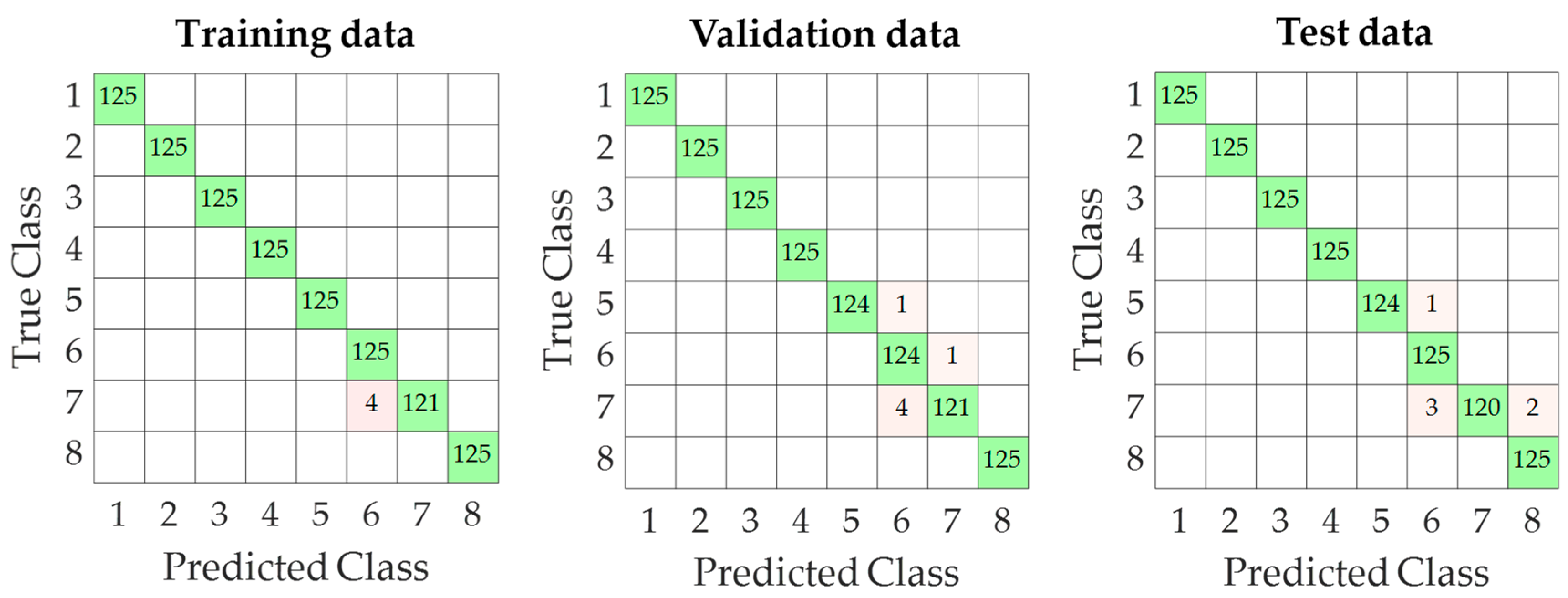
4. Experimental Verification of the Proposed Diagnostic Method

Verification of the neural structure in the training process is limited only to the analysis of the response of the network to the input information received in steady state. The tests were carried out for a wide range of voltages, fault types, and load characteristics. The results presented herein focus on the advantages of the proposed solution. Application under other conditions would require re-verification of the solution owing to the behavioural characteristics of the object (such as aircraft intermediate circuits).

From a practical point of view, it is important to validate the system in transient states and, above all, to evaluate the response of the system to a sudden change in the technical state of the object. Therefore, the final verification was carried out for capacitor faults modelled on the real object. This made it possible to determine the actual utility of the proposed diagnostic approach. Example test results for different supply voltage and load values are shown in Figure 14, Figure 15 and Figure 16.

An analysis of the verification results of the proposed diagnostic system shows that the proposed solution is highly dynamic (short response time to an emerging defect) and accurate. In the vast majority of cases, the result of the network coincides with the actual capacitance values of the capacitor used in the system. The result was determined in about 0.01 s, which was due to the use of 100 signal samples as input to the CNN and a signal acquisition frequency of 10 kHz. The time to determine the result was the same in all the cases studied, due to the fixed dimension of the input matrix, which translated into a fixed time for the acquisition of input data to the network, which is a major factor in the overall time of its operation, where the mentioned 0.01 s is the time of signal acquisition, while the time of calculating the response by the network was determined from the average of 1000 samples and amounted to 0.0101 s for 10,350 cases (i.e., for a single case less than 1 µs, for CPU Intel Core i7-13620 H and GPU NVIDIA GeForce RTX 4060, Santa Clara, CA, USA). However, it is worth mentioning that the algorithm works independently of the measurement, so detection occurs, at the latest, after the acquisition of 100 signal samples, but the study shows that the network allows detection even when the buffer is not full (which translates into an even shorter single detection time in the case of classification on an incomplete buffer).

It is also worth pointing out here the high versatility of the proposed solution, which, regardless of the load, was able to properly classify the capacitance value of the capacitor. Analyses were carried out not only for the cases shown in images 14–16. All available loads listed in Section 2.1 of the article, namely R, RL1, and RL2, were presented. The input voltages shown were limited to three values, marginal and middle (14 V, 32 V, and 51 V), but tests were also carried out for input voltages of 23 V and 41 V. The tests did not show an effect of load or input voltage on the dynamics and precision of the network response. Furthermore, for each combination of input voltage, load, and capacitor state (that is, specific capacitance), measurements were made by collecting 4000 samples. This gave 120 different configurations of 4000 samples each and for these, the nearly 100% efficiency of the proposed network was calculated. However, the classification of the fault itself is not as important as its detection; hence, it can even be determined that the network had 100% detection efficiency, assuming that a drop below 80% of the capacitor’s nominal capacitance is perceived as a fault. Due to the great limitation of the possibility of continuous physical modelling of capacitor damage for different stages of damage, the input information of the network was developed by combining the signals measured for different degrees of defect. Hence, rapid and large changes in the network’s predicted capacitances could be observed when these signals were combined. Such a response of the network is caused by the mixing of signals, which, when introduced into the aforementioned buffer of 100 samples, create input matrix combinations unprecedented by the network, which are difficult to classify. Such errors are especially visible at the highest supply voltage, for any type of load, and at the smallest capacitor damage, and for the RL₂ load, they are also visible for the presented supply voltage of 32 V (Figure 16). A simple and effective solution may be to use several network responses over an assumed time interval and, from this, infer the condition of the capacitors. This will not significantly increase the already short fault response time, but will eliminate false diagnostic information obtained from the network output.

However, significant in terms of proper network operation, there may be fluctuations in the response for λ = 84.87% for the lowest value of the input voltage. Detailed analysis has found that they are caused by slight differences between the signals for λ = 84.87% and λ = 90.40% at the aforementioned input voltage value (which can also be confirmed by the single misclassification observed between 0.035 and 0.135 s for the RL₁ load and λ = 90.40%). However, in each of the cases presented, the classification closes within the appropriate margin of error, without indicating that the capacitor is defective (assuming that a capacitor is considered defective when its capacitance drops below 80%); that is, without introducing the false negative. However, the high sensitivity of the proposed solution is worth pointing out here, which, despite small changes in capacitance at a low value of the supply voltage, can show a decrease in the capacitance of the capacitor under test. Another important finding is that the network does not maintain a detected change in the capacitance of the capacitor, but can demonstrate a healthy capacitor state again based on the provided measurements. This is important for the robustness of the solution to data transmission errors, where, if the results are sustained, the network, based on corrupted data, could incorrectly classify the capacitor state and sustain the misclassification, leading to incorrect conclusions and unnecessary failure prevention actions. As a result, incorrect classifications of individuals due to corrupted data will not affect the system’s performance.

5. Conclusions

The approach to capacitor fault diagnosis presented in this paper using transfer learning of a deep convolutional network ensures full exploitation of the Simulink-designed model. The paper demonstrates the high precision of the features learnt for the object model during verification of the real object for different operating and loading conditions of the system. It should be clearly emphasised that the proposed approach was based on the direct processing of raw signals by a convolutional neural network. As a result, the developed application was characterised by almost 100% precision in the assessment of the technical condition of the object and a very short response time to emerging defects of about 10 ms. Additionally, the use of automatic symptom extraction based solely on a Simulink-designed model eliminates the need for physical damage modelling to understand the physical phenomena that occur during damage. This fact is extremely important in the case of electrical faults, where intervening in the system to damage it is a risk. In the present study, the lowest classification value achieved was 16.8% of the nominal capacity, but this was dictated solely by hardware limitations, while the main training process was performed on simulation data, so the network could be adjusted to the selected capacities. The developed diagnostic system can provide an alternative to the currently used methods for assessing the condition of capacitors in power supply systems for electric drives.

References

1. Clean Hydrogen Joint Undertaking. Strategic Research and Innovation Agenda 2021–2027; Clean Hydrogen Partnership: Brussels, Belgium, 2021. [Google Scholar]
2. Undertaking, Clean Hydrogen Joint. 1st Call for Proposals: List and Description of Topics. In Annex to CAJU-GB-2022-03-16 Amended Work Programme and Budget 2022–2023; Clean Aviation Joint Undertaking: Brussels, Belgium, 2022. [Google Scholar]
3. HECATE—Hybrid Electric Regional Aircraft Distribution Technologies. Available online: https://hecate-project.eu/ (accessed on 20 December 2023).
4. Wolfgang, E. Examples for failures in power electronics systems. In Proceedings of the ECPE Tutorial on Reliability of Power Electronic Systems, Nuremberg, Germany, 19–20 April 2007. [Google Scholar]
5. Yang, S.; Bryant, A.; Mawby, P.; Xiang, D.; Ran, L.; Tavner, P. An industry-based survey of reliability in power electronic converters. IEEE Trans. Ind. Appl. 2011, 47, 1441–1451. [Google Scholar] [CrossRef]
6. Wang, H.; Blaabjerg, F. Reliability of capacitors for DC-link applications in power electronic converters—An overview. IEEE Trans. Ind. Appl. 2014, 50, 3569–3578. [Google Scholar] [CrossRef]
7. Wechsler, A.; Mecrow, B.C.; Atkinson, D.J.; Bennett, J.W.; Benarous, M. Condition monitoring of DC-link capacitors in aerospace drives. IEEE Trans. Ind. Appl. 2012, 48, 1866–1874. [Google Scholar] [CrossRef]
8. Hannonen, J.; Honkanen, J.; Strom, J.-P.; Karkkainen, T.; Raisanen, S.; Silventoinen, P. Capacitor aging detection in a DC–DC converter output stage. IEEE Trans. Ind. Appl. 2016, 52, 3224–3233. [Google Scholar] [CrossRef]
9. Yu, Y.; Zhou, T.; Zhu, M.; Xu, D. Fault diagnosis and life prediction of dc-link aluminum electrolytic capacitors used in three-phase ac/dc/ac converters. In Proceedings of the IEEE Second International Conference on Instrumentation, Measurement, Computer, Communication and Control, Harbin, China, 8–10 December 2012; pp. 825–830. [Google Scholar] [CrossRef]
10. Gao, J.; Huang, D.; Lu, J. Online output capacitor monitor for buck dc-dc converter. In Proceedings of the IEEE Prognostics and System Health Management Conference (PHM-Chongqing), Chongqing, China, 26–28 October 2018; pp. 802–806. [Google Scholar] [CrossRef]
11. Abdennadher, K.; Venet, P.; Rojat, G.; Retif, J.-M.; Rosset, C. A real-time predictive-maintenance system of aluminum electrolytic capacitors used in uninterrupted power supplies. IEEE Trans. Ind. Appl. 2010, 46, 1644–1652. [Google Scholar] [CrossRef]
12. Buiatti, G.M.; Martín-Ramos, J.A.; Garcia, C.H.R.; Amaral, A.M.R.; Cardoso, A.J.M. An online and noninvasive technique for the condition monitoring of capacitors in boost converters. IEEE Trans. Instrum. Meas. 2009, 59, 2134–2143. [Google Scholar] [CrossRef]
13. Laadjal, K.; Sahraoui, M.; Cardoso, A.J.M. On-line fault diagnosis of DC-link electrolytic capacitors in boost converters using the STFT technique. IEEE Trans. Power Electron. 2020, 36, 6303–6312. [Google Scholar] [CrossRef]
14. Aeloiza, E.; Kim, J.H.; Enjeti, P.; Ruminot, P. A real time method to estimate electrolytic capacitor condition in PWM adjustable speed drives and uninterruptible power supplies. In Proceedings of the IEEE 36th Power Electronics Specialists Conference, Dresden, Germany, 16 June 2005; pp. 2867–2872. [Google Scholar] [CrossRef]
15. Pu, X.S.; Nguyen, T.H.; Lee, D.-C.; Lee, K.-B.; Kim, J.-M. Fault diagnosis of DC-link capacitors in three-phase AC/DC PWM converters by online estimation of equivalent series resistance. IEEE Trans. Ind. Electron. 2012, 60, 4118–4127. [Google Scholar] [CrossRef]
16. Andrade, J.M. Electrolytic Capacitor Degradation Monitoring Using an On-Line Parameter Estimation Scheme involving Sliding Mode Differentiators and a Kalman Filter. In Proceedings of the IEEE 21st European Conference on Power Electronics and Applications (EPE’19 ECCE Europe), Genova, Italy, 3–5 September 2019; p. P-1. [Google Scholar] [CrossRef]
17. Zhang, W.; He, Y.; Wang, X.; Chen, J. A Comprehensive Method for Online Switch Fault Diagnosis and Capacitor Condition Monitoring of Three-level T-type Inverters. IEEE Trans. Power Electron. 2023, 38, 10183–10195. [Google Scholar] [CrossRef]
18. Meng, T.; Zhang, P. An on-line dc-link capacitance estimation method for motor drive system based on intermittent active control strategy. In Proceedings of the IEEE Energy Conversion Congress and Exposition (ECCE), Vancouver, BC, Canada, 10–14 October 2021; pp. 5118–5123. [Google Scholar] [CrossRef]
19. Bartlett, E.B.; Uhrig, R.E. Nuclear Power Plant Status Diagnostics Using an Artificial Neural Network. Nucl. Technol. 1992, 97, 272–281. [Google Scholar] [CrossRef]
20. Witczak, M. Advances in Model-Based Fault Diagnosis with Evolutionary Algorithms and Neural Networks. Int. Appl. Math. Comput. Sci. 2006, 16, 85–99. [Google Scholar]
21. Kobayashi, T.; Simon, D.L. Hybrid Neural-Network Genetic-Algorithm Technique for Aircraft Engine Performance Diagnostics. J. Propuls. Power 2005, 21, 751–758. [Google Scholar] [CrossRef]
22. Kowalski, C.T. Diagnostyka Układów Napędowych z Silnikiem Indukcyjnym z Zastosowaniem Metod Sztucznej Inteligencji; Oficyna Wydawnicza Politechniki Wrocławskiej: Wrocław, Poland, 2013. [Google Scholar]
23. Goodfellow, I.; Bengio, Y.; Courville, A. Deep Learning; MIT Press: Cambridge, MA, USA, 2016. [Google Scholar]
24. Fernandes, F.E.; Yen, G.G. Automatic Searching and Pruning of Deep Neural Networks for Medical Imaging Diagnostic. IEEE Trans. Neural Netw. Learn. Syst. 2020, 32, 5664–5674. [Google Scholar] [CrossRef]
25. Yang, H.; Wang, P.; An, Y.; Shi, C.; Sun, X.; Zhang, X.; Wie, T.; Ma, Y. Remaining useful life prediction based on denoising technique and deep neural network for lithium-ion capacitors. eTransportation 2020, 5, 100078. [Google Scholar] [CrossRef]
26. Kozma, R.; Ilin, R.; Siegelman, H.T. Evolution of Abstraction Across Layers in Deep Learning Neural Networks. Procedia Comput. Sci. 2018, 144, 203–213. [Google Scholar] [CrossRef]
27. Ince, T.; Kiranyaz, S.; Eren, L.; Askar, M.; Gabbouj, M. Real-Time Motor Fault Detection by 1-D Convolutional Neural Networks. IEEE Trans. Ind. Electron. 2016, 63, 7067–7075. [Google Scholar] [CrossRef]
28. Chattopadhay, P.; Saha, N.; Delpha, C.; Sil, J. Deep Learning in Fault Diagnosis of Induction Motor Drives. In Proceedings of the Prognostics and System Health Management Conference, Chongqing, China, 26–28 October 2018. [Google Scholar] [CrossRef]
29. Afrasiabi, S.; Afrasiabi, M. Real-Time Bearing Fault Diagnosis of Induction Motors with Accelerated Deep Learning Approach. In Proceedings of the 10th International Power Electronics, Drive Systems and Technologies Conference (PEDSTC), Shiraz University, Shiraz, Iran, 12–14 February 2019. [Google Scholar] [CrossRef]
30. Skowron, M. Development of a universal diagnostic system for stator winding faults of induction motor and PMSM based on TL. In Proceedings of the IEEE 14th International Symposium on Diagnostics for Electrical Machines, Power Electronics and Drives (SDEMPED), Chania, Greece, 28–31 August 2023. [Google Scholar] [CrossRef]
31. Skowron, M.; Kowalski, C.T. Permanent Magnet Synchronous Motor Fault Detection System Based on TL Method. In Proceedings of the 48th Annual Conference of the IEEE Industrial Electronics Society, Brussels, Belgium, 17–20 October 2022. [Google Scholar] [CrossRef]
32. Shao, S.; McAleer, S.; Yan, R.; Baldi, P. Highly accurate machine fault diagnosis using deep transfer learning. IEEE Trans. Ind. Inform. 2018, 15, 2446–2455. [Google Scholar] [CrossRef]
33. Wen, L.; Li, X.; Li, X.; Gao, L. A new transfer learning based on VGG-19 network for fault diagnosis. In Proceedings of the IEEE 23rd International Conference on Computer Supported Cooperative Work in Design (CSCWD), Porto, Portugal, 6–8 May 2019. [Google Scholar] [CrossRef]
34. Jigyasu, R.; Shrivastava, V.; Singh, S.; Bhadoria, V. Transfer learning based bearing and rotor fault diagnosis of induction motor. In Proceedings of the 2nd International Conference on Advance Computing and Innovative Technologies in Engineering (ICACITE), Greater Noida, India, 28–29 April 2022. [Google Scholar] [CrossRef]
35. MATLAB/Simulink Simscape Electrical Documentation. Available online: https://www.mathworks.com/help/sps/ (accessed on 18 April 2024).
Figure 1. Detailed schematic diagram of the voltage converter.
Electronics 13 01638 g001
Figure 2. Schematic diagram of the system to measure currents I1 and I2.
Electronics 13 01638 g002
Figure 3. Schematic diagram of the UB voltage measurement system.
Electronics 13 01638 g003
Figure 4. Experimental set-up—real view.
Electronics 13 01638 g004
Figure 5. Capacitor impedance and its components in the frequency domain [11].
Electronics 13 01638 g005
Figure 6. Simulink model diagram.
Electronics 13 01638 g006
Figure 7. Comparison of simulation measurement data obtained under different load conditions. (a) UB voltage, (b) I2 current.
Electronics 13 01638 g007
Figure 8. Comparison of simulation measurement data obtained under different power supply voltages. (a) Mean UB voltage, (b) mean I2 current.
Electronics 13 01638 g008
Figure 9. Comparison of simulation measurement data obtained under DC-link capacitance values. (a) UB voltage, (b) I2 current.
Electronics 13 01638 g009
Figure 10. Comparison of simulation and measurement signals. (a) UB voltage, (b) I2 current.
Electronics 13 01638 g010
Figure 11. Schematic diagram of TL.
Electronics 13 01638 g011
Figure 12. CNN training process for classic (simulation) and TL: (a) validation accuracy; (b) validation loss.
Electronics 13 01638 g012
Figure 13. Confusion matrices for training, validation, and test sets.
Electronics 13 01638 g013
Figure 14. Combined current signal and respective CNN responses for different voltages, for R load.
Electronics 13 01638 g014
Figure 15. Combined current signal and respective CNN responses for different voltages for the RL1 load.
Electronics 13 01638 g015
Figure 16. Combined current signal and respective CNN responses for different voltages, for RL2 load.
Electronics 13 01638 g016