Hardware/Software Co-Design of a Traffic Sign Recognition System Using Zynq FPGAs

Abstract

Traffic sign recognition (TSR), taken as an important component of an intelligent vehicle system, has been an emerging research topic in recent years. In this paper, a traffic sign detection system based on color segmentation, speeded-up robust features (SURF) detection and the k-nearest neighbor classifier is introduced. The proposed system benefits from the SURF detection algorithm, which achieves invariance to rotated, skewed and occluded signs. In addition to the accuracy and robustness issues, a TSR system should target a real-time implementation on an embedded system. Therefore, a hardware/software co-design architecture for a Zynq-7000 FPGA is presented as a major objective of this work. The sign detection operations are accelerated by programmable hardware logic that searches the potential candidates for sign classification. Sign recognition and classification uses a feature extraction and matching algorithm, which is implemented as a software component that runs on the embedded ARM CPU.

1. Introduction

Emerging technologies, such as vehicle-to-vehicle communications (V2V) [1], in-car cellular (online) connectivity [2] and increased computational prowess of embedded processors, are heralding a revolutionary change in car design and driver assistance systems. These technologies will play a key role in the development of self-driving cars in the near future [3,4]. A key component of advanced driver assistance systems is traffic sign recognition (TSR) that enables the car to recognize the road signs in real-world environments. Successful detection and recognition of traffic signs can be used to alert the driver and/or to facilitate autonomous driving operations. The main challenge for robust detection performance comes from the complexity of the environment, such as lighting conditions, weather conditions, similar color background and occlusions. A reliable and robust TSR system that can overcome those cases/circumstances should be considered as a priority. Besides reliability, real-time operation is another challenge for the TSR system. A system that can provide sign information even at high traveling speeds is necessary for driver assistance systems.

In this work, a new TSR algorithm flow is proposed, which performs exceptionally robustly against environmental challenges, such as partially-obscured, rotated and skewed signs. Another critical component is the embedded system implementation of the algorithm on a programmable logic device that can enable real-time operation. The proposed work is based on earlier research [5,6], which introduced a programmable hardware platform for TSR. This study shares the sign detection steps, but introduces a new sign recognition algorithm based on feature extraction and classification steps and its corresponding hardware implementation.

In general, TSR systems are comprised of two parts: sign detection and sign recognition/classification. Many approaches for sign detection are based on color space information. In [7], a summary is given for color space threshold methods, including the RGB normalized threshold [8], the hue saturation threshold [9], the hue saturation enhancement threshold [10] and the space threshold [11]. For sign recognition [12], several feature extraction methods have been proposed, including Canny edge detection [13], scale invariance feature (SIFT) [14] and, more recently, speeded-up robust feature (SURF) [15]. HOG (histogram of oriented gradients) can also be used as features, as shown in [16,17]. Typically, features are extracted for the subsequent machine learning stage, which is used for the sign classification. Support vector machine (SVM) [18] and neutral networks [19] are popular classifiers based on such techniques.

In recent years, a great variety of hardware solutions for real-time TSR has been proposed. These include conventional (general purpose) computers [20], custom ASIC (application-specific integrated circuit) chips [21], field programmable gate arrays (FPGAs) [22,23,24,25], digital signal processors (DSPs) [26] and also graphic processing units [27]. Although it is difficult to make a direct comparison due to differences in the TSR algorithms employed, the following section discusses the motivation and outcomes of these hardware architectures with respect to the proposed hardware/software solution.

In [20], a software-based solution running on a Linux system with a 2.4-GHz dual core CPU is presented. The algorithm implements color processing and feature matching and is shown to have 95% accuracy. However, their traffic sign set is limited to only 20 signs, and the PC platform is not an embedded system that can be integrated into a car. In [21], a low power 0.13-μm ASIC chip has been presented for traffic sign detection, incorporating an image enhancement preprocessor and a sign recognition preprocessor. The image enhancement preprocessor uses the MSR (multi-scale retinex) algorithm, providing a robust image, adaptable to light and dark conditions. It uses neural-fuzzy logic to control the parameters of the MSR algorithm, and the recognition processor uses a support vector search engine for classification. Although the chip performs well, it is considered to be a very costly solution due to the inflexibility of the ASIC platform for any post-silicon changes. FPGAs, on the other hand, provide unlimited reconfigurability as a hardware platform, and they are increasingly popular choices for TSR implementations. In [22], a SURF detector has been implemented on Kintex-7 FPGA, which is claimed to achieve a frame rate at 60 fps at 800 × 600 resolution. However, no information regarding the traffic sign recognition algorithm or relevant detection performance are given in the paper. The architecture given in [23] uses HOG features and the SVM classifier. The classification accuracy is 93.77%. However, the absence of any preprocessing step (sign detection) in the algorithm makes it difficult to recognize a potential sign in a raw image, and the effective accuracy is lower. Another FPGA architecture given in [24] uses a multi-core SoC implementation, targeting a latency of less than 600 ms (maximum latency for a car traveling at a speed of 180 km/h). Specifically, a Gaisler/Pender Electronics FPGA board, GR-CPCI-XC4V [28], is used for hosting a dual core LEON-3 processor and realizing a dedicated hardware accelerator for the support vector machine kernel used in the TSR algorithms. This is a very expensive prototype board and not feasible for production purposes. In [25], a TSR system is implemented on a Spartan-6-FPGA and includes color-based sign detection and feature-based classification steps, similar to our work, but their system is only capable of detecting speed limit signs. Many industry TSR solutions, such as cars manufactured by BMW and Mercedes, are also limited to speed limit signs [29]. In [26], an automated sign detection algorithm has been implemented using a TI OMAP L138 DSP chip. The DSP solution is shown to achieve an execution time of 300 ms for both detection and recognition parts. However, the recognition part is based on template matching, which would generally fail for tilted, rotated and partially-obscured traffic signs, unlike the feature matching algorithm in our proposed system. Finally, a GPU (graphical processor unit)-based solution is proposed in [27]. At the software level, the authors have used parallel processing to improve the efficiency of computing. An average frame rate of 21 fps is achieved by the GPU (~50-ms latency), which presents a good alternative to FPGAs due to the programmability of GPUs, but generally, the cost and power consumption of GPUs are very high.

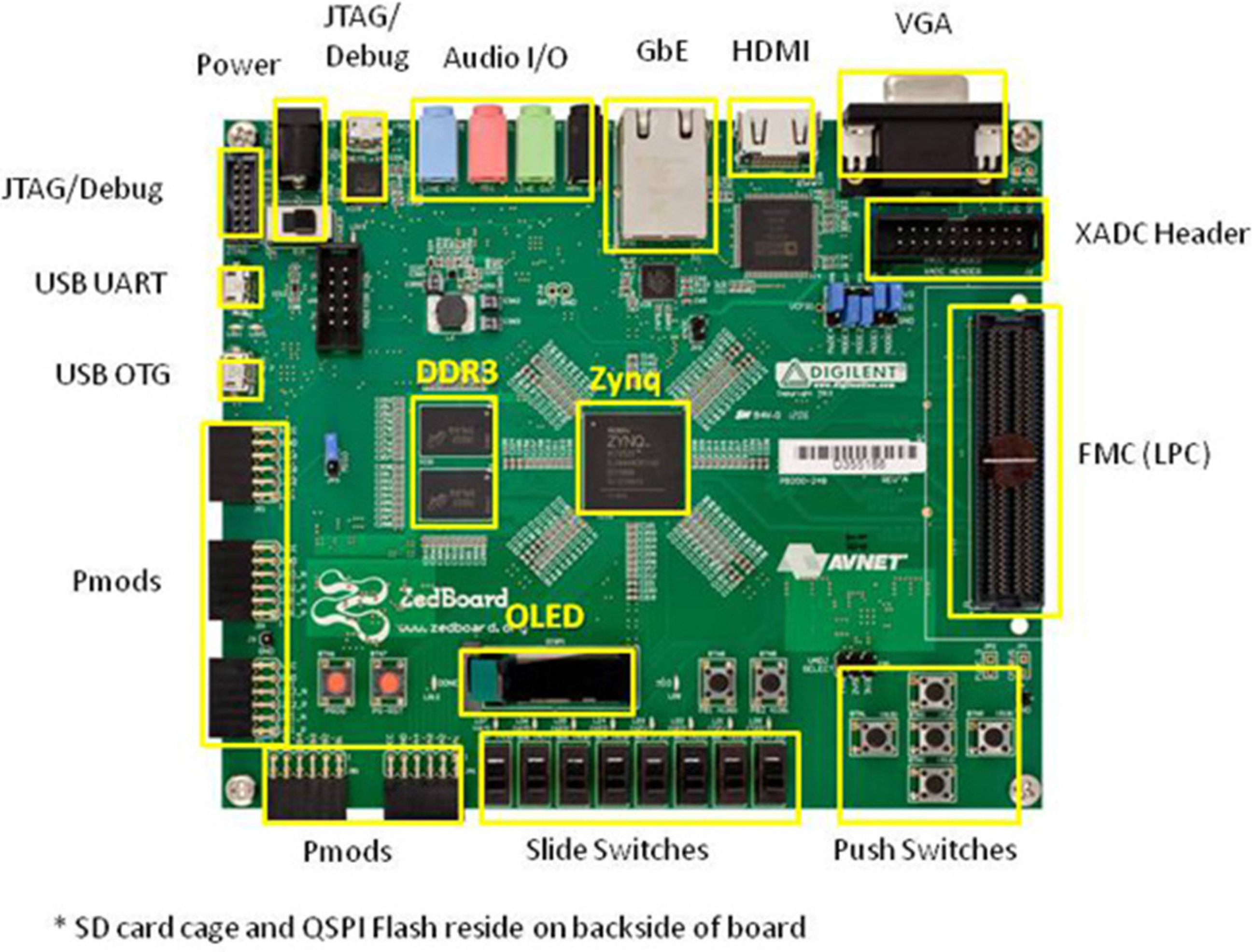
The TSR system presented in this work is unique due to a balanced approach in the software and hardware components. TSR algorithm has robust recognition performance (i.e., tolerates rotated, tilted, shifted and even obscured signs); it supports all traffic signs (not just speed limit signs); it can be easily expanded to different regional traffic sign sets (belonging to different countries or states) by training; and it is computationally efficient. The target hardware platform, the Zynq FPGA, is a low cost, low power and flexible system that provides fast development due to embedded ARM processor cores and the reconfigurable logic blocks. It can also be integrated into automotive embedded systems.

The rest of the paper is organized as follows: In Section 2, color-based sign detection is described, and the SURF detection algorithm is introduced. New feature extraction methods are explained. Section 3 discusses the FPGA platform and the system components. Finally, experimental results for evaluating the detection accuracy are shown in Section 4, and hardware performance results are given.

2. Algorithm Overview

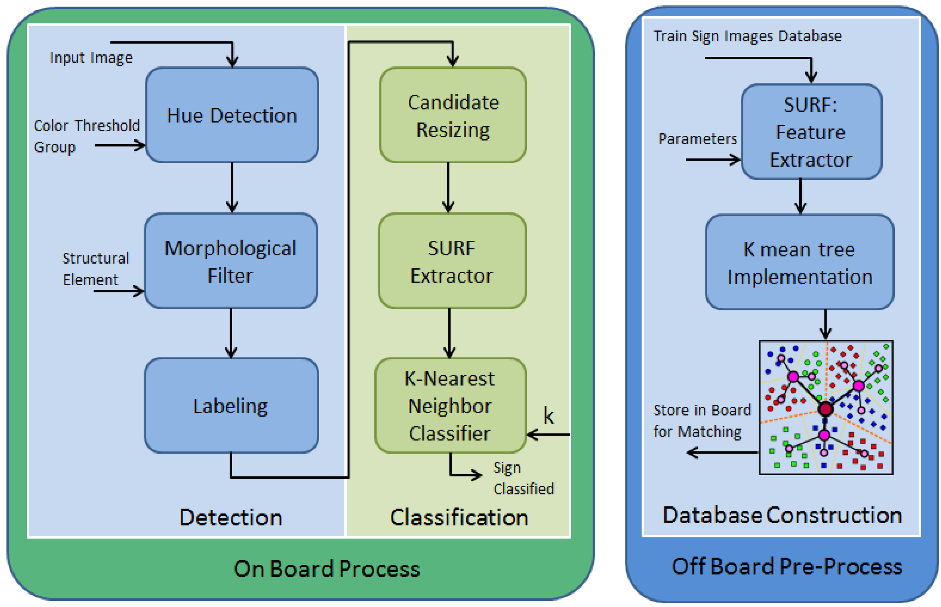
The task of traffic sign recognition can be divided into two sub-tasks of detection and classification. Detection is the response of finding the region of interest that could contain a traffic sign. Classification takes the challenge of identifying if these candidates are truly traffic signs and classifying them. Figure 1 presents the proposed algorithm used for sign detection and classification. The main goal of this work is to design a fast, robust and reliable TSR system. To overcome the challenges mentioned above, the algorithms are chosen carefully. The presentation of the image is transferred from the RGB space to the hue/saturation/intensity space to achieve lighting invariance. To make the system invariant to rotation and skew, the SURF detector is adopted to extract the feature for matching. To achieve real-time sign recognition, an FPGA-based implementation is utilized in order to map the entire algorithm into hardware acceleration. As shown in Figure 1, the algorithms implemented as hardware acceleration include hue detection, morphological filter, labeling and scaling, while feature extraction and nearest neighbor search are done on an embedded CPU core.

Figure 1. System flowchart for the proposed traffic sign recognition (TSR) algorithm. The green section (left) highlights detection and classification operations executed on an embedded system (FPGA). The blue section (right) shows the training steps executed on a PC.

Figure 1. System flowchart for the proposed traffic sign recognition (TSR) algorithm. The green section (left) highlights detection and classification operations executed on an embedded system (FPGA). The blue section (right) shows the training steps executed on a PC.

The original input image is transferred from the RGB domain to the HSI (hue, saturation and intensity) domain. By mapping the values with the hue color wheel in HSI, pixels can be categorized as a particular color, such as red or yellow. Then, morphological filters (opening and closing steps) are applied, which are used to eliminate the noise from the single or small group of red pixels. The rest of the positive pixel groupings are labeled as the potential signs. The labeling process identifies a square block for each and every pixel grouping in the image. The labeled pixel groupings are candidates for possible traffic signs. Among these candidates, most of them are too small, that they may not contain enough information for candidate matching. Hence, these non-feasible candidates need to be filtered out by calculating their height and width. Only those candidates that contain enough resolution are considered as good candidates. The subsequent steps deal with the second part of the TSR algorithm: the sign classification part. The possible traffic sign candidates are scaled into a certain resolution, and features are extracted by the SURF detector. These features are used to perform nearest neighbor search (or other machine learning algorithms) with the training database for classification. If the matching condition is satisfied, it will be classified as the equivalent traffic sign. The algorithms mentioned above are implemented on a Xilinx FPGA board. An example of the off board process required to prepare the database for sign classification is shown in Figure 1. Training images are captured for feature extraction. To accelerate the searching speed, the features are constructed into a k-means tree structure and stored in the board. The following sections provide more details about the algorithms.

2.1. Color-Based Segmentation

Sign detection is primarily finding the region of interesting (ROI) that may contain signs. One of the most popular methods is color-based segmentation. A traffic sign is usually designed with a single background color, e.g., red, yellow or blue, which can be easily distinguished from the environment. Images are usually displayed in the RGB color model, in which red, green and blue light are combined together to reproduce a broad array of colors. RGB is very useful when displaying colors and widely used in our input/output devices, like cameras, scanners and color TV. Using RGB directly is considered as the simplest way for color segmentation. However, the three color components used to present red, green and blue pixels are highly correlated and also easily affected by illumination conditions. The same color, under different saturation levels or light, may cause an almost random variance of RGB values.

2.1.1. Color Detection

In this paper, color-based segmentation in the HSI space is taken. HSI represents a pixel by its hue, saturation and intensity. The hue component describes the color itself in the form of an angle between [0, 360] degrees. Zero degrees means red; 120 means green; 240 means blue; 60 degrees is yellow; 300 degrees is magenta. The saturation component signals how much the color is polluted with white color. The range of the S component is [0, 1], if the RGB value has been normalized to [0, 1]. The Intensity range is between [0, 1], and zero means black and one white, if the RGB value has been normalized to [0, 1].

Given an image in RGB format, the H component of each pixel is obtained using the equation [30]:

$$H= \{\begin{array}{c}\theta if B\le G\\ 360°-\theta if B \ge G\end{array}$$

(1)

with:

$$\theta = {\cos }^{-1}\left\{\frac{\frac{1}{2}\left[\left(R-G\right)+\left(R-B\right)\right]}{{\left[{(R-G)}^2+\left(R-B\right)\left(G-B\right)\right]}^{\frac{1}{2}}}\right\}$$

(2)

A fast version is given by [31]:

$$H= \{\begin{array}{c}\begin{array}{c}0, R=G=B\\ \frac{\left(G-B\right)60°}{max\left(R,G,B\right)-min\left(R,G,B\right)}mod 360°, R\ge G,B\end{array}\\ \begin{array}{c}\frac{\left(B-R\right)60°}{max\left(R,G,B\right)-min\left(R,G,B\right)}+120°, G\ge R,B\\ \frac{\left(R-G\right)60°}{max\left(R,G,B\right)-min\left(R,G,B\right)}+240°, B\ge R,G\end{array}\end{array}$$

(3)

The saturation and intensity can be calculated by equation [32]:

$$S=1- \frac{3}{\left(R+G+B\right)}\left[\min \left(R,G,B\right)\right]$$

(4)

$$I=\frac{1}{3}\left(R+G+B\right)$$

(5)

Once the conversion is made, the hue values for each pixel can be used for detection. Detection is the process of identifying a pixel whose hue value falls in a certain range of the hue wheel. Then, the image can be split into two components: pixels that have the color of interest and those that do not. A binary image can be created by flagging each pixel as to whether it belongs to the color of interest or not. According to [7], the red, yellow, blue and white colors can be detected by the following Equation (6) with the thresholds listed in Table 1:

$$Pixel\left(i,j\right)=\{\begin{array}{c}Red, if H\left(i,j\right)\le Th{R}_1 \\ or H\left(i,j\right) \ge Th{R}_2 \\ \\ Blue, if H\left(i,j\right)\ge Th{B}_1 \\ and H\left(i,j\right)\le Th{B}_2\\ \\ Yellow, if H\left(i,j\right)\ge Th{Y}_1\\ and H\left(i,j\right)\le Th{Y}_2 \\ and S\left(i,j\right)\ge Th{Y}_3\\ \\ White, if S\left(i,j\right) \le Th{A}_{ } \\ and I\left(i,j\right)\ge Th{W}_{ }\\ \\ Else, otherwise\end{array}$$

(6)

Table 1. Color detection thresholds [7].

Color	Threshold Values
Red	$Th{R}_1=10, Th{R}_2=300$
Blue	$Th{B}_1=190, Th{B}_2=270$
Yellow	$Th{Y}_1=20, Th{Y}_2=60, Th{Y}_3=150$
White	$Th{A}_{ }= 48, Th{W}_{ }=60$

Table 1. Color detection thresholds [7].

Color	Threshold Values
Red	$Th{R}_1=10, Th{R}_2=300$
Blue	$Th{B}_1=190, Th{B}_2=270$
Yellow	$Th{Y}_1=20, Th{Y}_2=60, Th{Y}_3=150$
White	$Th{A}_{ }= 48, Th{W}_{ }=60$

2.1.2. Morphological Filters

In the binary image created above, not all pixels are part of the traffic signs. Much spark noise sometimes spreads on the image. Leaving them without any processing will only cause them to propagate to the next level and harm the detection performance. Hence, the image has to be filtered. For this spark noise, such as single dots or small pixel blobs, a morphological filter is an easy and efficient way to remove those pixels and only leave larger candidates for the next step.

The basic idea of the binary morphological filter is to sweep an image with a window called the structuring element (SE), which is a pre-defined small geometric window, such as a square or cross. There are two basic operators: erosion and dilation. Other operators, such as opening and closing, are sequential combinations of these two operators. Erosion is good enough to eliminate those small pixel blobs, but it also trims other objects. Opening meets the requirement of eliminating the noise and retaining the information of other objects. The remaining object(s) could be treated as a region of interest that may contain a traffic sign. In this work, different structural elements have been tried, as shown in Figure 2. Large structure elements may cause the loss of a potential sign; and multiple combinations of erosion and dilation operations improve the results slightly. Therefore, the conclusion was that a single opening operation (erosion and dilation) with a 3 × 3 square structure element provides the best results.

Figure 2. Experimental results of morphological filters with various combinations of operations and structural elements. Clockwise from top left corner: original image; after erosion and dilation steps using 3 × 3 pixel structural elements; after erosion and dilation steps using 5 × 5 pixel structural elements; after erosion, dilation, dilation and erosion steps using 3 × 3 pixel structural elements.

Figure 2. Experimental results of morphological filters with various combinations of operations and structural elements. Clockwise from top left corner: original image; after erosion and dilation steps using 3 × 3 pixel structural elements; after erosion and dilation steps using 5 × 5 pixel structural elements; after erosion, dilation, dilation and erosion steps using 3 × 3 pixel structural elements.

2.1.3. Labeling

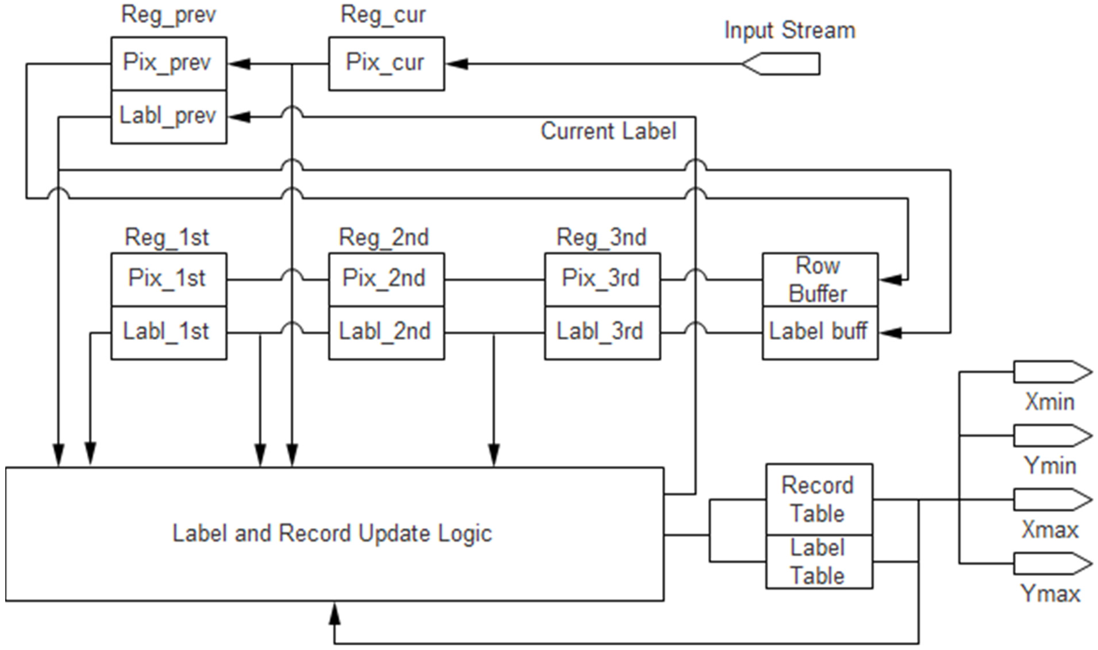
Labeling is the process of scanning the image to detect pixel groupings. Pixels that share an edge or a vertex are considered to be members of the same pixel grouping or “blob”. The remainder of this section details the algorithm used to detect these blobs. The goal with labeling is to identify a bounding box for each and every pixel grouping in the image. This will result in four parameters for every blob: X_min, Y_min, X_max, Y_max. These are the two diagonal corners that define the bounding box. Simply put, the labeling algorithm scans the image from bottom to top and left to right (raster order) keeping track of X_min, Y_min, X_max and Y_max for all of the pixel groupings it encounters. During this scanning, only one row plus two pixels are stored and labeled at a time in memory. Labels are assigned, and a table is built containing the X_min, Y_min, X_max and Y_max values for each label. While scanning, a window of five pixels is examined at a time: the current pixel and its four previously-visited neighbors. The window size is chosen to be five due to the reduced memory usage (only one row plus two pixels). Each pixel initially starts with a label of 0 (not labeled), and if the pixel is a foreground pixel, then a non-zero label is assigned. The value of that label depends on the labels of its four neighbors.

Figure 3 shows all of the possible combinations for consideration when determining the label of the current pixel. Each of these diagrams represents the current pixel, X, its immediate previously-scanned neighbor, P, and its previously-scanned neighbors, 1, 2 and 3. Shaded pixels are active and labeled. There are two special cases distinguished by the red and blue borders. The first special case, marked in red, is the case in which none of the current pixel’s neighbors have a label. In this case, the current pixel receives a new label. The second special case, marked in blue, is the case when the current pixel has multiple neighbors that have labels, and these labels may not be the same. When different labels meet at the current pixel, relabeling must happen, so that a single bounding box is generated to encompass what had been two separate labels. The remaining case is the simplest: the current pixel has one or more previously-labeled neighbors having the same label. In this case, the current pixel is simply labeled in kind.

Figure 3. Possible pixel configurations for the labeling process. X is the current pixel; P is the immediate previous neighbor; 1, 2 and 3 are previously-scanned neighbors [5].

Figure 3. Possible pixel configurations for the labeling process. X is the current pixel; P is the immediate previous neighbor; 1, 2 and 3 are previously-scanned neighbors [5].

While pixel labels are being assigned, the bounding box for each label is being grown to encompass all of the pixels that contain that label. This is done by maintaining a record table that holds X_min, Y_min, X_max and Y_max for each label. The second special case described above is where the interesting portions of this algorithm reside. When two labels meet, the algorithm is discovering for the first time that what was previously thought to be two distinct blobs is indeed one. The records that have been maintained thus far will need to be updated to include this information. One possible approach would be to rescan all or portions of the image. However, given that doubling back to reliable portions of the image can be a time-consuming step, it was chosen to solve this problem by using a level of indirection. Each pixel is given a label. This label does not point to a record of X_min, Y_min, X_max and Y_max, but rather, to a record number. This record number points to these actual bounding box parameters. In this way, when two labels meet, both labels can be made to point to the same record that will now encompass what was once two labeled groupings.

Consider the example in Figure 4. This is a simple 16 × 16 pixel image that contains two blobs that should be labeled by the labeling algorithm. As the algorithm begins, as shown in Figure 4a, the first three pixels encountered are labeled with new labels, as they have no labeled neighbors that have been encountered yet. The pixels that are marked with red indicate this special case; a new label is used. The record table to the right shows the values it would take at this point in the scan of the image. The next two figures (Figure 4b,c) show what happens when Labels 1 and 2 meet and when Labels 2 and 3 meet. The yellow box shows the window the algorithm is considering at that point in time. When two labels meet, the label table is updated to point to the lower record entry. This entry is also updated, so that the points it describes encompass all of the pixels of both labels. In this way, information is carried along. Figure 4d shows the fully-labeled image with its completed record table. It can be seen that temporary label numbers, 1, 2, 3, all point to the same record number and boundary box as expected, since they belong to the same “blob”.

Figure 4. Labeling example. (a). Three new labels are created; (b) Labels 1 and 2 meet; (c) Labels 2 and 3 meet; (d) completed labeling. Labels 1, 2 and 3 all point to the same record number and boundary box.

Figure 4. Labeling example. (a). Three new labels are created; (b) Labels 1 and 2 meet; (c) Labels 2 and 3 meet; (d) completed labeling. Labels 1, 2 and 3 all point to the same record number and boundary box.

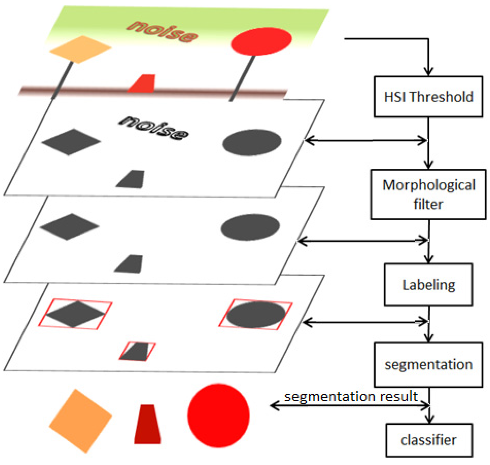
Figure 5. Detection of potential traffic signs. Steps include RGB to HSI conversion, denoising using morphological functions, labeling (grouping) of potential signs and extraction of potential signs to be forwarded to the sign classifier process.

Figure 5. Detection of potential traffic signs. Steps include RGB to HSI conversion, denoising using morphological functions, labeling (grouping) of potential signs and extraction of potential signs to be forwarded to the sign classifier process.

2.1.4. Segmentation and Detection of Traffic Sign Candidates

After the labeling step, multiple regions of interest (each label corresponds to an ROI) have been identified and extracted, and they are sent to the sign classification part. This is accomplished by mapping the associated binary image with the original image. The associated binary image is the result of the original image processed by all steps mentioned above. Coordinates provide the location of the ROI, and active binary pixels provide the exact pixels that need to be extracted from the original image. Figure 5 shows the complete procedure for the detection of traffic sign candidates.

2.2. Sign Classification

After the sign detection step, several regions of interest are obtained that may potentially contain a traffic sign. Next, these potential signs are searched in the traffic sign database in order to find a match. In this work, a sign classification approach based on speeded-up robust features (SURF) [33] and the nearest neighbor classifier is used. The SURF detector is used to detect and extract features from hundreds of sign templates for training. The nearest neighbor classifier is used in the final step for categorization.

2.2.1. Feature Extraction and SURF Detector

SURF is a robust local feature detector popular in computer vision applications. It is based on the SIFT algorithm and is shown to be faster and more robust against SIFT. It uses the determinant of the Hessian matrix to find interest points. For a continuous function of x and y, the value of the function at $(x, y)$ is given by $f(x,y)$. The Hessian matrix H of function $f$ at $(x, y)$ is:

$$H\left(f\left(x,y\right)\right)=\left[\begin{array}{cc}\frac{{\partial }^{2}f}{\partial x^2}& \frac{{\partial }^{2}f}{\partial x\partial y}\\ \frac{{\partial }^{2}f}{\partial x\partial y}& \frac{{\partial }^{2}f}{\partial y^2}\end{array}\right]$$

(7)

where $\frac{{\partial }^{2}f}{\partial x^2}$, $\frac{{\partial }^{2}f}{\partial y^2}$ and $\frac{{\partial }^{2}f}{\partial x\partial y}$ are second partial derivatives of function $f$.

The determinant of this matrix is given as:

$$\det \left(H\right)=\frac{{\partial }^{2}f}{\partial x^2}\frac{{\partial }^{2}f}{\partial y^2}-{\left(\frac{{\partial }^{2}f}{\partial x\partial y}\right)}^2$$

(8)

This determinant is used to estimate whether the function f has extremum at $(x, y)$. If the determinant is positive, which means f changes with x and y in the same direction, then point $(x, y)$ could be a local extremum. If the determinant is negative, which means f changes with $x$ and $y$ in different directions, then point $(x, y)$ is not a local extremum.

For image processing, we can just replace the function $f(x, y)$ by a gray image $I(x, y)$. The second order derivative can be replaced by the Laplacian. Since Laplacian is sensitive to noise, the SURF detector combines the Gaussian filter for smoothing. Then, the second order derivative is replaced by the Laplacian of Gaussians (LoG).

SURF features are scale invariant. To achieve this, scale-space is used to find the extrema across all possible scales. Typically, this is achieved by creating an image pyramid with smaller down-sampled images. For computational efficiency, instead of using an image pyramid, SURF increases the size of the filter to achieve a similar effect. Based on the response of these filters, a scale-space is created. A non-maximal suppression is performed in a 3 × 3 × 3 neighborhood to localize interesting points. The interest point localized by the determinant of the Hessian matrix is compared against its 26 neighbors. If it is greater than its surrounding pixels, it is selected as a maximum. After locating the interest points, descriptors are created using the Harr wavelet response of the surrounding pixels. Each interest point is assigned an orientation. If descriptor components of an interest point are extracted relative to this orientation, it will be invariant to image rotation. In order to determine the orientation, Haar wavelet responses in the x and y direction are calculated for a set of sampled points within a radius of 6σ at the detected interest point, where σ refers to the scale at which the interest point was detected.

2.2.2. Dataset, Feature Selection and Training

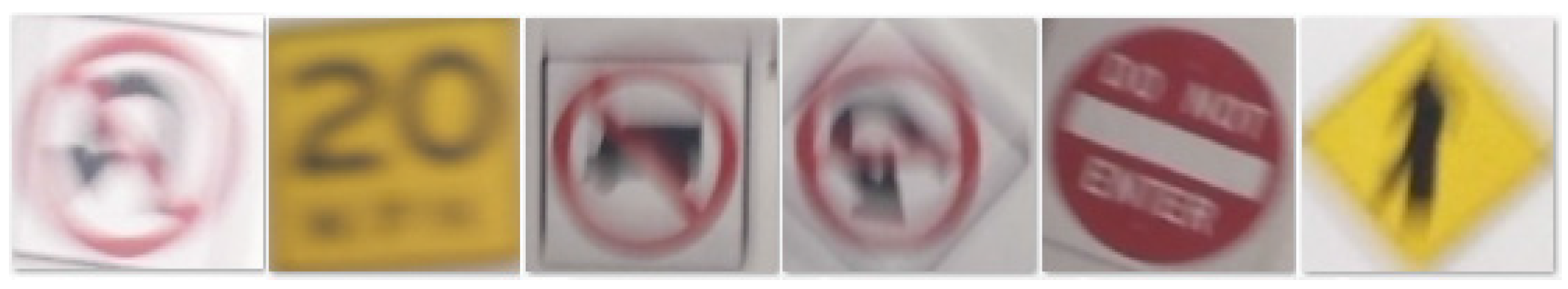
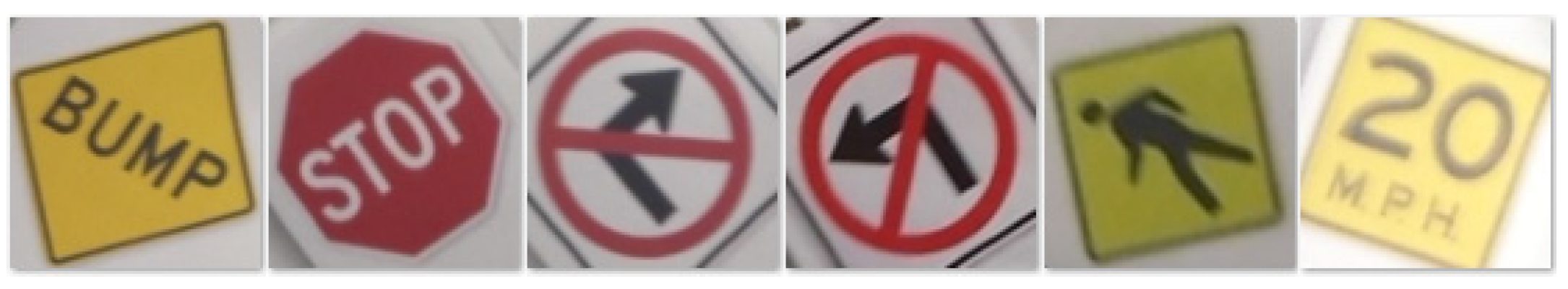
The SURF detector is used to find a reliable extractor that could provide robust features to the traffic sign database for machine learning. One problem for feature extraction is the difficulty of finding a suitable database that contains enough examples of U.S. traffic signs sampled from a natural environment. Collecting examples from different sources is not desirable, since various brands of camera plus various image formats will make the database unreliable for testing and training. Therefore, we created a sign database by taking hundreds of signs with different rotation and scale values. The numbers of signs with different color categories are listed in Table 2. Some example images are shown in Figure 6.

Figure 6. Example images from the traffic sign dataset.

Figure 6. Example images from the traffic sign dataset.

Table 2. Distribution of primary colors in the sign dataset.

Sign Color	Number of Signs
red	8
yellow	13
white	12

Table 2. Distribution of primary colors in the sign dataset.

Sign Color	Number of Signs
red	8
yellow	13
white	12

Figure 7 shows an example traffic sign, “BUMP”, with detected interest points. It can be seen that some of the interest points are detected at the edge. In fact, there are as many interest points at the edge as the interest points detected around the center. Center interest points usually contain more valuable (distinguishing) information. Most signs in our database contain edges that contribute a large number of redundant interest points to our database. Furthermore, using this database for training leads to undesirable outcomes. To avoid the disturbance of those interest points around edges and to reduce the number of interest points, we propose two feature selection methods for database creation. One method is to setup a threshold of the determinant of the Hessian matrix at the interest point detection step. Recall the determinant function, where $\frac{{\partial }^{2}f}{\partial x^2}$ and $\frac{{\partial }^{2}f}{\partial y^2}$ are second derivatives of function f in the x and y direction, respectively. Both $\frac{{\partial }^{2}f}{\partial x^2}$ and $\frac{{\partial }^{2}f}{\partial y^2}$ will have larger values, if point(x, y) is of the corner. 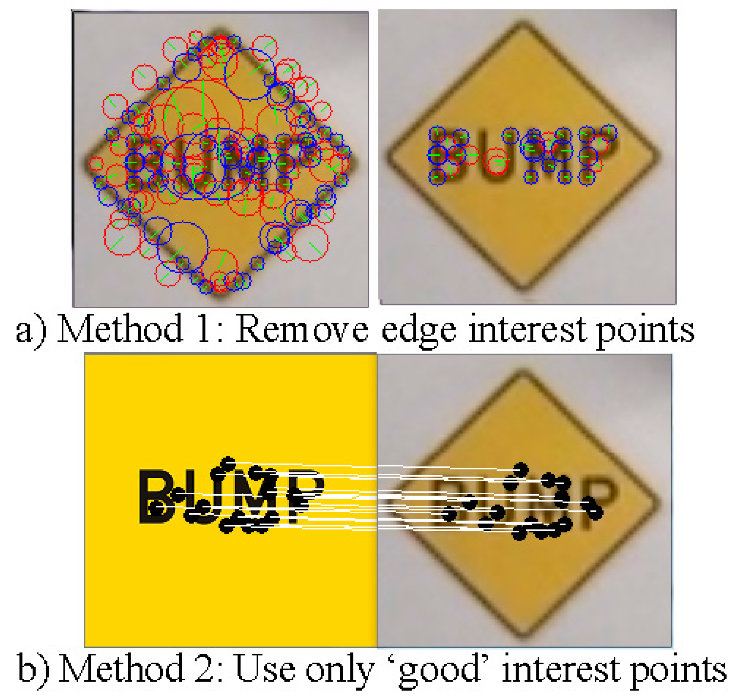If the point (x, y) is of the edge, then either $\frac{{\partial }^{2}f}{\partial x^2}$ or $\frac{{\partial }^{2}f}{\partial y^2}$ would like to have a larger value. Hence, the determinant of the points around the corner is larger than the determinant of the points around the edge. Based on the experimental results, a threshold value is selected. The interest points detected after thresholding (interest points at the edges are ignored) are shown in Figure 8a.

Another method is to cut off the edges from training images and then extract only “good” matches from the remainder image (see Figure 8b). For each interest point of the query image, we calculate its distance with every interest point in the template image and find the minimum distance and second minimum distance. Generally, a good match has both a smaller absolute distance and smaller relative distance. Hence, a determinant of a good match is given by:

$$(\frac{d_1}{d_2}<T_1) and (d_1<T_2)$$

(9)

where $d_1$ is the minimum distance, $d_2$ is the second minimum distance, $T_1$ is the relative threshold and $T_2$ is the absolute threshold. This equation was validated by experimental results. To balance the number of interest points of each sign, $T_1$ and $T_2$ can be adjusted during the extraction processing.

Figure 7. Detected interesting points (features) on a traffic sign image for “BUMP”.

Figure 7. Detected interesting points (features) on a traffic sign image for “BUMP”.

Figure 8. Proposed interest point reduction methods for database creation. (a) Method 1: removal of interest points around the edge; (b) Method 2: select only “good” interest point matches.

Figure 8. Proposed interest point reduction methods for database creation. (a) Method 1: removal of interest points around the edge; (b) Method 2: select only “good” interest point matches.

The similarity measure between two interest point p and q is based on Euclidean distance, which is given by:

$$d=\sqrt{{\left(q_1-p_1\right)}^2+{\left(q_2-p_2\right)}^2+\cdots +{\left(q_{64}-p_{64}\right)}^2}$$

(10)

Figure 9 shows the flowchart of the feature database creation. For Method 1, interest point matching is not required. The determinant threshold, which can eliminate edge points, needs to be set before executing the program. The program is designed to build only one type of traffic sign at a time. Once the program starts, a single training image will be loaded, then features will be extracted and stored. The program will extract features iteratively until all images (belonging to one traffic sign) are done. The final step will be combining these features extracted from different images together and storing in a single file “database”.

As described earlier, Method 2 uses only features from training images that have “good” matches on the template image. Hence, an extra matching step is inserted to create the database for Method 2, as shown in Figure 9b. Since features of a single image have been extracted in the previous process, the program starts from read features form “sign_name_i ipts” files. The standard template will be treated as the target sign, and features from other training images will try to find their match on this template sign. The iteration will keep executing until all images are done. The final step is to store all matched features in a single file. For both programs, the final database contains features extracted from 33 different types of traffic signs (set from Illinois, USA).

Figure 9. Flowchart for database creation. Repeat the steps for each traffic sign. Training can be done with any number of test images. (a) Method 1 uses the determinant threshold to eliminate edge interest points; (b) Method 2 determines the “good” matches to a template image and only uses those interest points as features.

Figure 9. Flowchart for database creation. Repeat the steps for each traffic sign. Training can be done with any number of test images. (a) Method 1 uses the determinant threshold to eliminate edge interest points; (b) Method 2 determines the “good” matches to a template image and only uses those interest points as features.

2.2.3. k-NN Classification

In pattern recognition applications, the k-nearest neighbor is a non-parametric method used for classification and regression. In k-NN classification, the output is a class membership. An object is classified by a majority vote of its neighbors, with the object being assigned to the class most common among its k-nearest neighbors, If k = 1, then the object is simply assigned to the class of that single nearest neighbor. It has been proven that the risk of 1-NN is never more than twice the value of the Bayes risk [34].

The training examples are vectors in a multidimensional feature space, each with a class label. The training phase of the algorithm consists of only storing the feature vectors and assigning labels of the training samples. In the classification phase, k is a user-defined constant, and a query is classified by assigning the label that is most frequent among the k training samples nearest to that query point.

The easiest way of searching the nearest samples is exhaustive search or brute force search. In this algorithm, each query point is compared to all training points in the database. Searching the closest matches to high-dimensional vectors in a large database will lead to a computationally-expensive problem. Instead of using exhaustive search, our database is transferred into a k-means tree structure. Once the tree is constructed, the searching problem becomes tracing a branch to find a leaf and comparing with every points inside the leaf to find the nearest points. Again, the Euclidean distances are calculated for the similarity measure. If the distance is smaller than the threshold, it will be considered as a good match. The sign that contains the highest number of good matches will be treated as a potential positive detection. If this number is greater than the threshold and it occupies 30% of the total number of good matches, it will be considered as a positive detection, and the traffic sign is identified. The 30% threshold is to avoid those noises that may have broad matches among different signs. Figure 10 shows the sign classification flow with the database creation described above.

Figure 10. Sign classification based on SURF and nearest neighbor search.

Figure 10. Sign classification based on SURF and nearest neighbor search.

3. FPGA Implementation

In this section, an FPGA-based TSR system implementation is described. The sign detection part has been successfully realized as a custom IP core [5]. The sign classification based on template matching and k-NN classification is designed as software code running on the ARM CPU embedded in a Zynq FPGA.

3.1. Development Environment

The TSR system has to be able to provide the traffic sign information as a car approaches the sign. Then, the execution time of the algorithm becomes an issue. Generally, the hardware implementation is necessary due to timing requirements. However, some operations or some types of data may increase the complexity of the hardware design. If possible, a compromise between hardware and software is desirable. In this scheme, the software component is used to pre-process data and communicate with hardware blocks. For example, MicroBlaze is an embedded soft core processor, optimized for implementation on Xilinx FPGAs. It has advanced architecture options, like an AXI or PLB interface, a memory management unit, instruction and data-side cache, a floating-point unit, and more. Figure 11 shows our earlier TSR design using the MicroBlaze soft core [5]. The MicroBlaze was initially used to handle the input and output data streams, setup parameters for the image processing peripheral and implement some portions of the image processing algorithm [5]. Since MicroBlaze is soft core, it has vast flexibility. There are many options for configuring the soft core according to the performance and resource utilization requirements. The key drawback of the MicroBlaze soft core system was the limited clock frequency of the programmable logic. The RAM access during the application programming is also inconvenient, which increases the complexity of development. To fill the market requiring more powerful embedded system development tools, Xilinx released Xilinx Zynq-7000, which contains a dual 1-GHz ARM Cortex-A9 processor that comes with a high performance memory system. ZedBoard is a complete development kit for designers using the Zynq-7000 All programmable SoC. As shown in Figure 11 [5], this board includes all of the necessary interfaces and peripherals to enable a wide range of applications.

Figure 11. System block diagram [5].

Figure 11. System block diagram [5].

One of the key goals of this work is to develop an efficient combination of a software processing system (C code running on CPU cores) and an FPGA logic for hardware acceleration and control. Compared to the MicroBlaze CPU, the ZedBoard processing system, shown in Figure 12, runs much faster, and it is not necessary to add and manage a RAM unit. It has 512 Mb DDR3 attached, which is large enough for most of the applications. ZedBoard provides an efficient combination of a processing system (software) and FPGA. The development of custom IP cores is more like a plug-and-play design. A framework was designed based on this stimulus, as shown in Figure 13 [6]. Xilinx’s Embedded Development Kit (EDK) was used to create this platform, which includes blue and red parts, as shown in the figure. The processing system includes the ARM cores, which are responsible for running the program on top. The red part is the interface AXI4 and its attached registers, the back-bone of the whole system. It carries the responsibility of communications among the processing system, hardware peripherals and PC. Registers attached to customer peripherals (once they are created) are software accessible. This means parameters can be sent to the peripherals by writing simple codes to set these registers. These registers could be classified as a control register, a status register, a data register and an address register. The control register is used to initialize the peripheral. The data register is used to transfer data, and the address register is used to set a proper IP buffer address for data register, which means the data in the data register will be transferred into the IP buffer associated with the address register. Overall, the interface is very intuitive. Since software-accessible register drivers will be automatically generated, EDK has been used to create the custom IP. The debug window is like an HCI, which is used to display the interaction of applications. The processing system handles the input and output data. The system uses UART to build the connection to the PC. AXI4 interface is used to build the connection between the CPU processing system and hardware peripherals. The proposed system was implemented on a Xilinx ZedBoard as a HW/SW co-design.

Figure 12. ZedBoard and peripherals [35].

Figure 12. ZedBoard and peripherals [35].

Figure 13. FPGA system framework (adapted from Han and Oruklu [6], with permission from © 2014 IEEE).

Figure 13. FPGA system framework (adapted from Han and Oruklu [6], with permission from © 2014 IEEE).

3.2. Hardware Implementation

3.2.1. Hue Calculation and Detection: Hardware IP Core

Generally, the hardware has its advantage in processing data streams. Hence, the image is transferred as a stream of pixels in RGB format. As described in the previous section, the image is converted into the HSI color spectrum. The hue value represents the color; the saturation represents the purity of the color; and intensity represents how dark that color is. Hence, only hue calculation should be good enough to detect the color. Unfortunately, there is no such hue value for the white sign. In this situation, saturation and intensity have to be calculated. Compared to the hue calculation, determining the saturation and intensity is much easier. Figure 14 shows the implementation of hue calculation in the hardware. The circuit takes in the RBG values and outputs hue values. The division step requires 17 clock cycles to fill the pipeline and generates the quotient every clock cycle. Hence, it is necessary to introduce delay registers that allow the control signals, offsets and quotient to align.

Figure 14. Hue calculator logic.

Figure 14. Hue calculator logic.

According to Equation 2, the hue value should be a value between zero and 359. To simplify the multiplication, 64 (a power of two) degrees are used as the multiplier, rather than multiplying by 60 degrees [31]. This resulted in a color wheel with a range between zero and 383. Furthermore, the red color has a zero value in the original color wheel. To avoid the modulo calculation for red pixels, the color wheel is rotated by 64 degrees. This can be achieved by implementing the offset according to the following equation:

Offset = 256·Bmax + 128·Gmax + 64

(11)

3.2.2. Morphological Filtering: Hardware IP Core

Figure 15 shows the hardware implementation of morphological filters, which can be used for both erosion and dilation. Single-bit registers are used to hold the pixels within the filter window, which is also called a structural element. The enabled signal is attached to the output of each register to make the structural elements programmable. The filter window is implemented as a 5 × 5 rectangle. Therefore, it is not necessary to redesign the combination logic when the structural element changes. Further, the duality relation between erosion and dilation enables both to be implemented with a single circuit. A control signal E/_D is used to complement both input and output signals. This increases the flexibility of the design and allows for reuse when different combinations of filters are needed. The center of the window is the pixel under evaluation. Combinational logic compares the central pixel and its neighbors to determine if the output pixel should be active or inactive. Given that the image arrives as a data stream, a row buffer has to be attached to hold all of the pixels in a row. Therefore, when the filter window scans the image, the pixels stored in the buffer can be piped to the filter. Since a 5 × 5 filter window is chosen, four row buffers are required.

Figure 15. Morphological filter implementation.

Figure 15. Morphological filter implementation.

According to experimental results, a structural element of a 3 × 3 square and a single open operation gives the cleanest image, while not Hamming the traffic sign. This is based on the image with a resolution of 320 × 240. If the resolution of the image increases, a larger structural element may be needed to adapt to the changes.

3.2.3. Labeling: Hardware IP Core

Similar to the morphological filter process, labeling also requires a window to scan the binary images. The five pixels in the window, as mentioned in Section 2, are the current pixel and its four previous visited neighbors. A pixel buffer and a label buffer are required to hold pixels and labels, respectively. Figure 16 shows the block diagram for the labeling circuit. The label and record update logic block determine the labels for each pixel and update the label and record table. If the current pixel is active, a label will be assigned to that pixel. It is determined by which case gets hit (see Figure 3).

Figure 16. Labeling implementation.

Figure 16. Labeling implementation.

At the end of the labeling process, an acknowledgement will be received by the software part indicating that the segmentation is done, and the labeling results are ready to be loaded.

3.2.4. Candidate Resizing: Embedded CPU Program

At this stage of the TSR algorithm, the boundaries of potential candidates have been extracted and loaded by the ARM CPU for sign classification. Before executing the classification algorithm, the candidates need to be further processed. A small box may not contain enough information for classification, and a big box has no chance to be a traffic sign. Those candidates that are too small or big could be easily removed by calculating the X_max-X_min and Y_max-Y_min. After this, only those candidates with a proper size remain. Each candidate has to be scaled to a certain resolution based on the method of classification. So far, two classification methods have been implemented on the ZedBoard. One method is to directly match the template pixel by pixel. Another method is based on the nearest neighbor classifier. For the template matching method, each candidate will be scaled to the same resolution as the template and then compared to each template. For the nearest neighbor classifier, each candidate will be scaled to 200 × 200 pixels, and then, features will be extracted. For both methods, the scaling algorithm calculates the ratio between the original size of the candidate and the target resolution. A new memory location is used as the storage location of the new resized candidate. The algorithm locates and scans the candidate on the original image based on its boundaries and sets the pixels of the scaled candidate to be active or inactive according to the calculated ratio.

3.3. Classification Implementation: Embedded CPU Program

The SURF detector has been implemented on many platforms, such as the OpenCV library and MATLAB. However, our bare-metal system can only run pure C/C++ code plus basic C/C++ library. Hence, OpenSURF [36], which is given in nearly pure C++ code, is adopted and converted to a C version that can run on an ARM processor. The OpenSURF still uses the OpenCV library to load the image and stores in Mat format, which is primarily used by the OpenCV function. In the C library, we only have the array or matrix that can be used as the image container. During the implementation, it was found that the matrix created by the “malloc” function does not work properly, which left “array” as the only choice. All of the function calls or use of the Mat container have been transferred to proper ones. OpenSURF also uses the OpenCV library to perform the last step in localizing the interest point, whereas our implementation uses the Gaussian elimination algorithm.

For sign recognition, as described in Section 2, features are extracted from training images and stored in a file. This database will be loaded to the ZedBoard before sign detection. To find the best matches in the database, each feature calculates its Euclidean distance. Once the distance meets the condition, a good match is counted. The sign that contains the highest number of good matches will be treated as a potential positive classification.

4. Accuracy Analysis and Performance Results

4.1. Experimental Results

For initial accuracy performance analysis, experiments are carried out on a PC, using Visual Studio 2010 with OpenCV library Version 2.49 and OpenSURF. Our image database includes 33 types of signs and thousands of test images in total. Experiments are categorized into three database groups, Group 1, Group 2 and Group 3, depending on the feature selection and interest point reduction method. In order to make a comparison, the images used for extracting interest points for each group are the same.

For Group 1, No interest point reduction strategy is used.

For Group 2, feature selection Method 1 is used; no interest points around the edges.

For Group 3, feature selection Method 2 is used; only interest points that have a good match are used.

The accuracy results are listed in Table 3 and Figure 17. The accuracy results are represented in two ways: (1) misclassification rate and (2) false classification rate. The misclassification (MC) represents the signs that are detected in the sign detection stage, but neglected and not classified into any category in the sign classification stage. False classification (FC) represents the signs that are detected in the sign detection stage, but classified to the wrong category. Most of the false recognitions are caused by blurry images (shown in Figure 18), which do not contain enough good features for matching. For actual applications, false classification is more critical than misclassification. The camera may capture dozens of frames per second; and most misclassified signs may be eventually correctly recognized. On the other hand, FC errors cannot be recovered from. Considering that FC is more critical than MC, both Group 2 and Group 3 databases have better results. The Group 3 database (generated using Method 2) has the least FC. All groups perform robustly for rotated and skewed signs, as shown in Figure 19 and Figure 20, respectively.

Table 3. Accuracy analysis for SURF feature extraction and nearest neighbor search.

	Group 1 Database	Group 2 Database	Group 3 Database
Number of training images	231	231	231
Number of test images	1236	1237	1218
Misclassification (MC)	7.69%	5.74%	11.82%
False classification (FC)	3.80%	2.18%	0.99%

Table 3. Accuracy analysis for SURF feature extraction and nearest neighbor search.

	Group 1 Database	Group 2 Database	Group 3 Database
Number of training images	231	231	231
Number of test images	1236	1237	1218
Misclassification (MC)	7.69%	5.74%	11.82%
False classification (FC)	3.80%	2.18%	0.99%

Figure 17. Performance of test images with 20% blurry images and 30% rotated images. MC is misclassification; FC is false classification; and TF is total failure. Groups 1, 2 and 3 differ in their interest point selection for database creation.

Figure 17. Performance of test images with 20% blurry images and 30% rotated images. MC is misclassification; FC is false classification; and TF is total failure. Groups 1, 2 and 3 differ in their interest point selection for database creation.

Figure 18. Examples of blurry images.

Figure 18. Examples of blurry images.

Figure 19. Rotated sign examples.

Figure 19. Rotated sign examples.

Figure 20. Skewed sign examples.

Figure 20. Skewed sign examples.

If the blurry images are removed from the test images, the accuracy performance is greatly improved, as shown in Figure 21. Group 3 still has the best FC. Group 2 has the best overall performance in recognition. From the experiments, it was observed that signs with a similar layout have a higher false classification rate, such as “lane merge right” and “lane merge left”. The speed limit sign has the highest false classification rate. The speed limit signs for 30, 45 and 55 have similar layouts, except the number, which leads to a significant mixed boundary between their features. The larger mixed boundary will cause a higher false classification rate.

Figure 21. Performance of test images without blurred images. MC is misclassification; FC is false classification; and TF is total failure. Groups 1, 2 and 3 differ in their interest point selection for database creation.

Figure 21. Performance of test images without blurred images. MC is misclassification; FC is false classification; and TF is total failure. Groups 1, 2 and 3 differ in their interest point selection for database creation.

4.2. Hardware Performance Results

Table 4 compares the execution time of our earlier TSR algorithm running on Virtex 5 and ZedBoard platforms. This particular algorithm uses the same front end (HSI color space, morphological filters, labeling and scaling steps) and implements a simple template matching based on Hausdorff distance calculation, which is fast, but not very robust with respect to accuracy [5].

Table 4. Comparison of TSR algorithm performance running on Virtex 5 and Zynq FPGA platforms.

Algorithm Steps:	Execution Time:
	MicroBlaze and IP Cores on Virtex 5	ARM CPU and IP Cores on Zynq
Custom IP peripheral core: (HSI conversion, morphological filters, labeling)	114 ms	28.7 ms
Scaling and template matching (Hausdorff distance)	663.3 ms	67.8 ms
Total Time	777 ms	96.5 ms

Table 4. Comparison of TSR algorithm performance running on Virtex 5 and Zynq FPGA platforms.

Algorithm Steps:	Execution Time:
	MicroBlaze and IP Cores on Virtex 5	ARM CPU and IP Cores on Zynq
Custom IP peripheral core: (HSI conversion, morphological filters, labeling)	114 ms	28.7 ms
Scaling and template matching (Hausdorff distance)	663.3 ms	67.8 ms
Total Time	777 ms	96.5 ms

Next, the SURF-based feature extraction and matching algorithm is implemented on the ZedBoard FPGA hardware. A user-friendly PC interface in C# is designed for controlling the ZedBoard (shown in Figure 22). The terminal window presents all of the responses from the application, which displays the same information as the SDK terminal. The debug window displays the execution times of the SURF detector and search. Once the ZedBoard is initialized, the program running on the board loads the test image and waits for the command to execute the SURF detector. The open image button displays the image under test. Start SURF will trigger the ZedBoard to execute the SURF detector to extract features for matching. The classification results and timing results are shown on the left.

Figure 22. Execution time for the (recognition phase only) “CROSSWALK” sign using brute force matching.

Figure 22. Execution time for the (recognition phase only) “CROSSWALK” sign using brute force matching.

Figure 22 shows an example of brute force searching based on the database that only contains 10 signs. The number of features stored in the database is around 1500. The average classification time, which includes executing the SURF detector and brute force searching, is about three seconds. Figure 23 shows the timing performance of k-means search, which contains the complete Group 3 dataset that includes around 5000 features. As shown in the results, the matching time of k-means is much faster (less than a second) than the brute force template match, even if the number of features stored in the system is 3.3-times larger. Nevertheless, a 992-ms total execution time (shown in Table 5) cannot be considered as a real-time operation speed for fast moving cars. Therefore, the execution time of the SURF detector in particular needs to be improved by the hardware accelerator blocks instead of the software implementation.

Figure 23. Execution time for the (recognition phase only) “CROSSWALK” sign using k-means matching.

Figure 23. Execution time for the (recognition phase only) “CROSSWALK” sign using k-means matching.

Table 5. Performance results for the proposed TSR algorithm.

	Sign Detection (Hardware IP Cores for HSI Conversion, Morphological Filters, Labeling)	Sign Recognition and Classification (Runs on ARM CPU)
		SURF Feature Extractor	k-NN Search
Execution Time	28.7 ms	892 ms	72 ms
		964 ms
Total Time	992.7 ms

Table 5. Performance results for the proposed TSR algorithm.

	Sign Detection (Hardware IP Cores for HSI Conversion, Morphological Filters, Labeling)	Sign Recognition and Classification (Runs on ARM CPU)
		SURF Feature Extractor	k-NN Search
Execution Time	28.7 ms	892 ms	72 ms
		964 ms
Total Time	992.7 ms

Figure 24 shows the resource utilization of the target Zynq FPGA platform. Due to the software-only implementation of the SURF algorithm, only 30% of the logic slices are needed for the TSR hardware IP blocks. It is evident that more hardware peripherals can be instantiated to accelerate the feature extraction algorithm and achieving real-time operation.

Figure 24. FPGA hardware resource usage for the proposed TSR system.

Figure 24. FPGA hardware resource usage for the proposed TSR system.

5. Conclusions

In this paper, a new TSR system that combines the SURF feature extractor and nearest neighbor classifier methods has been presented. The system shows robust detection performance even for rotated or skewed signs. False classification rates can be reduced to less than 1%, which is very promising. The proposed TSR system that combines hardware and software co-design is implemented on Xilinx’s ZedBoard. An ARM CPU framework based on the AXI interconnect is developed for custom IP design and testing. Overall, the system throughput is eight times faster compared to the authors’ previous design based on the Virtex 5 FPGA, when considering both IP hardware execution and algorithms implemented in software. The current execution time of 992 ms may not be sufficient for real-time operation (when a fast moving car is considered); however, the FPGA resource usage is very low, and dedicated IP blocks can be used to implement the SURF algorithm and improve the computation time. This would enable real-time TSR. This hardware platform can be also expanded to include other driver assistance technologies that may be necessary in autonomous cars, such as pedestrian detection and lane detection, which utilize similar computer vision methods.