An SAR-ISAR Hybrid Imaging Method for Ship Targets Based on FDE-AJTF Decomposition


1
State Key Laboratory of Complex Electromagnetic Environment Effects on Electronics and Information System, Luoyang 471003, China
2
School of Graduate, Space Engineering University, Beijing 101416, China
3
Space Engineering University, Beijing 101416, China
*
Author to whom correspondence should be addressed.
Electronics 2018, 7(4), 46; https://doi.org/10.3390/electronics7040046
Submission received: 1 March 2018
/
Revised: 26 March 2018
/
Accepted: 29 March 2018
/
Published: 30 March 2018
Abstract
:In high-resolution spaceborne synthetic aperture radar (SAR), imaging of moving ship targets is strongly influenced by ships’ complex three-axis motions, so that imaging results are fuzzy and unfocused. Yet scattered and moving information on ship targets is wholly contained in the complex image data. This paper proposes a novel SAR and inverse SAR (SAR–ISAR) hybrid imaging method to improve imaging effects, using this complex SAR image data on ship targets, and based on frequency-domain-extraction-based adaptive joint time frequency (FDE–AJTF) decomposition. First, complex SAR image data is transformed to the Doppler domain in the azimuth dimension, and the optimum azimuth data are selected. Next, the signal in each range cell is decomposed to its polynomial phase signal (PPS) components by FDE–AJTF. Finally, a two-dimensional image of the ship target at a given azimuth time is constructed directly. The feasibility and effectiveness of this proposed imaging method is verified through comparisons with conventional methods in simulation and experimental tests.
1. Introduction
Ships are an essential ocean target that play important roles both in the civil and military fields. Spaceborne synthetic aperture radar (SAR) has obvious advantages in ship target surveillance on the vast ocean, due to its all-time and all-weather active imaging abilities. However, with improved SAR resolution and increases to the synthetic period, the unique echo features of a moving ship lead to a series of adverse effects [1]. Additionally, under normal sail, the ship’s motions have multiple periodicities and strong randomness, caused by the sea wind and waves, in three axes [2]. The influences of these complex motions are mainly in three aspects: first, the motions generate high-order non-cooperative phase errors in the echo signal which cannot be accurately compensated. Second, ship rotation leads to different movement characteristics of its scattering points, and as a result the envelope migrations are different in different range cells. Third, the Doppler echo is periodic and random, which results in the frequency folding and wrapping in the azimuth dimension. Solving these three issues is the key to obtaining a precise image of moving ship targets.
To date, there are two methods of moving target imaging. Conventionally, a target is processed through three steps: moving target detection, moving parameters estimation and compensation, and azimuth imaging. To achieve a high-resolution and well-focused image, multichannel techniques are necessary, such as displaced phase center antenna (DPCA) imaging [3], space-time adaptive processing (STAP) [4], and along-track interference (ATI) [5]. However, most current spaceborne SAR systems are single-channel and do not satisfy the multi-channel requirement; thus, these methods are not adaptively applied.
The second method, SAR–ISAR hybrid imaging, takes a secondary image by inverse SAR (ISAR), [6,7], and includes classical ISAR methods and time-frequency analysis methods. Due to the aforementioned problems caused by complex three-axis motions, the processing steps of envelope alignment and phase correction have few effects in the classical ISAR method. Nevertheless, time-frequency analysis can obtain clear two-dimensional images by analyzing the relationship between the scattering point location and the Doppler change in the echo phases, and there are three different means that can be adopted for imaging: polynomial phase compensation, range instantaneous Doppler (RID) imaging [8] and extracting scattering points by using CLEAN technology [9].
The high-resolution SAR echo of a moving ship can be expressed as a high-order multicomponent polynomial phase signal (mc-PPS) [10], which may contain severe envelope migration and Doppler wrapping. Under these circumstances, the classical time frequency analysis method cannot satisfy the processing requirements of mc-PPS. To process mc-PPS effectively, two methods are popularly adopted. The first is the maximum likelihood (ML) method, which can obtain the optimal solution via parameter estimation [11]. However, the application of the ML method is limited because of its multi-dimensional searching space and very large computation requirements. A modified quasi-ML (QML) method [12] has been proposed, which offers several improvements and is widely applied in the PPS process. A detailed review of QML is presented in reference [13]. The second generally adopted method is polynomial phase transformation (PPT) [14], whether discrete polynomial phase transformation (DPT) [15], high-order ambiguity function (HAF) [16], or cubic phase function (CPF) [17], etc., all of which can reduce the phase order based on phase differentiation (PD) and reduce the searching space to one dimension. These methods are influenced by the cross terms and their resolutions are limited by the PD process. Although many modified methods have been proposed to reduce the cross terms, such as the product forms of HAF (PAHF) [18] and CPF (PCPF) [19], these methods are also influenced by the cross terms of the mc-PPS, especially when numerous components are contained and the intensities of every component are similar. The PPT methods are reviewed in detail in Reference [20].
The adaptive joint time frequency (AJTF) method [21], as a modified ML method, is widely applied in ISAR imaging [22], if parameterized, it can represent the signal by extracting the signal components piece by piece and offer good resolution without the influence of cross terms when processing high-order mc-PPS. However, the classical AJTF methods have very large computation requirements, are easily influenced by noise and estimation errors, and cannot fit the time window of the signal component correctly. In addition, classical AJTF application in ISAR imaging assumes only two-dimensional motions of the target, which is not the case for targets with complex three-dimensional motions [23].
A frequency domain extraction-based AJTF (FDE–AJTF) decomposition method has been proposed, offering three improvements: estimation and extraction of the component in the frequency domain, the use of a time window on the basis function, and the adoption of CFAR detection in component extraction. These improvements increase the stability, speed, and accuracy of the components’ estimation and extraction [24].
Based on FDE–AJTF decomposition, we propose a novel SAR–ISAR hybrid imaging method to solve the high-resolution imaging problems presented by a moving ship. In this method, the moving ship area on the complex SAR image data is initially tailored and translated to the range-Doppler domain by Fourier transformation; then, the optimum azimuth data with well-aligned envelopes is selected and decomposed to PPS components by the FDE–AJTF method; and finally, a two-dimensional RID image is constructed from these PPS components of all range cells.
2. SAR–ISAR Hybrid Imaging
2.1. Optimum Azimuth Data Selection Method
The imaging process in a spaceborne SAR system is mature and solidified, but cannot deal with single ship targets individually. However, the motion and scattering features of a target ship are wholly contained in the SAR complex image, which makes secondary ISAR imaging possible.
The imaging principles of SAR and ISAR are essentially the same. After SAR imaging is done, the phase errors caused by the motions of the SAR platform are compensated for, though the phase errors caused by the ship’s motions endure, causing a fuzzy and unfocused image. Fortunately, these remaining phase errors are in the azimuth dimension, and the ship target area on the SAR image is easily recognized to the clear background of the sea. After the image data of the ship target is tailored and transformed to the Doppler domain, the signal in each range cell can be regarded as a mc-PPS, and can be estimated and compensated by time frequency analysis.
The complex motions of a ship not only influence the echo phase in the azimuth dimension, but also lead to envelope migration in the range dimension. Thus, envelope alignment is the first step in single-ship targeting, whether using SAR or ISAR imaging. However, the scattering points of a complex three-axis moving ship have different motion characteristics, so that their envelopes migrate without a uniform rule for the different range cells, which makes it difficult to align all envelopes at once. This problem is particularly acute when the near points affect each other.
ISAR imaging by time frequency analysis provides a solution that does not require all the azimuth data, only an optimum section in which well-aligned envelopes are selected for processing. Hence, two benefits are brought: these envelopes are well-aligned in the optimum section, which reduces the negative effects of envelope migration; and the complexity of the Doppler in the section is lower, with a shortened azimuth time and easier, more accurate parameter estimation.
To select the optimum section, the correlation characteristics between the two adjacent range cells can be used as the basis for judgment. The correlation characteristics generally include four indices: the inner product, i.e., the correlation value at zero drift, the mean and standard deviations of the inner products within a certain range cell window, and the peak drift of the correlation.
Assuming the signal in the rth range cell is , then the correlation of the rth and (r + 1)th range cells is as follows [25]:
where is the drift, and is the signal length.
The normalized inner product is the correlation value at zero drift, as follows:
The mean and the standard deviation of the inner products are as follows:
where is the window width on the range cells, and is the rectangular window.
The peak drift is the maximum value position in the correlations:
where gets the absolute value. To increase precision, interpolation is used in the calculation; here may be a decimal.
These four indices should be comprehensively considered to select the optimum azimuth data section, in which these conditions are satisfied: the inner products are high and smooth with high mean and low standard deviations and the peak drifts of the correlations are small. Only after the optimum azimuth data is selected can the ISAR imaging be processed well.
However, there is another problem in optimum azimuth data selection: the point number of the Doppler transformation. Tailoring a ship area on a completed SAR image is essentially a windowing process in the time domain, while optimum azimuth data selection is also another windowing process after transforming to the Doppler domain. According to the features of discrete signal Fourier transformation, the resolution and frequency range are closely related to the point number of the transformation [25]. The periodicity of the target ship’s three-axis motions generates a periodic Doppler in the echo, while the former two winnowing processes reduce the transform point number, which may result in Doppler folding and wrapping. To solve this problem, commonly the original complex image data is expanded by zero fill in the azimuth dimension before being transformed to the Doppler domain.
2.2. FDE–AJTF Decomposition Method
The echo signal for a range cell of a moving ship can be expressed as an mc-PPS, and one PPS component in the whole signal is as follows [24]:
where is the component intensity; is the rectangular time window of width , and the center point is zero; is a time-independent constant phase; is the linear term of time , which is related to the real position of the target scatter point; and and the higher-order parameters are related to the target motion, which leads to the phase error and should be compensated in the imaging process.
To estimate the parameters, a basis function is needed. The basis function for the FDE–AJTF method is the compensation phase function with a time window, as follows:
where is the time window and and are the window’s center and width, respectively. The time window is used to fit the real component time accurately. To simplify the analysis, the time window can be neglected.
The compensated signal is obtained by following process:
where is the basis function without a time window.
The image, that is, the frequency spectrum , is obtained by Fourier transformation, as follows:
where, is Fourier transformation. The maximum value of the spectrum is at , which is the scattering point image as a envelope function.
To get the best image, the fitness function is the maximum spectrum value , as follows:
where are the estimating parameters and is the peak position .
The spectrum peak is a envelope function, and its main lobe is distributed in the neighborhood of . The estimated component is extracted in the frequency domain by extracting the main lobe; meanwhile, the residual signal is updated by wiping off the main lobe as follows:
where is the residual signal in the frequency domain and is the neighborhood range. The minimum neighborhood is ; the robustness can be increased by extending the neighborhood range properly.
Then, the extracted component can be represented as follows:
where is the component intensity which is the main lobe energy of .
The residual signal in the time domain can be obtained by multiply the inverse Fourier transformation of and the conjugate of the compensation phase function, as follows:
where is the inverse Fourier transformation; the is the conjugate of the compensation phase function with parameters .
The other components can be extracted from the residual step by step, and finally the signal can be represented as follows:
where is the component number and is the residual after components are extracted.
In the FDE–AJTF decomposition method, the optimization algorithms, such as the genetic algorithm (GA) [26], particle swarm optimization (PSO) algorithm [27], ant colony optimization (ACO) [28], etc., are used to accelerate the parameter searching speed, and the constant false alarm ratio (CFAR) is applied in the component extraction to filter clutter and noise and to increase imaging effectiveness [29]. As an example, in the simulation and experimental test of this paper, the PSO algorithm is used in the parameters searching.
2.3. Image Construction
Using RID imaging, after obtaining the time-frequency distributions (TFDs) at all azimuth times of all the range cells and distributing them across the three dimensions of time, frequency, and range, the two-dimensional RID image can be obtained by extracting a certain azimuth time slice of the TFDs of all the range cells [8]. However, in this process we need to calculate the three-dimensional TFDs at all times of all ranges, resulting in a very large computation for which not all calculations are used. To reduce computation demands and improve efficiency, an image construction method is proposed to directly construct only the RID image at a particular time, by which method the display resolution and scale can be easily controlled.
The TFD of a single component signal converges to the instantaneous frequency curve with a probability of 1, whereas the phase of the PPS is continuously differentiable. Therefore, the instantaneous frequency of a single component can be calculated directly without any cross terms. According to Equation (12), the instantaneous frequency is calculated as follows:
where are the estimated parameters. This instantaneous frequency is the basis of TFD.
The frequency and range scales to display should be determined first. In discrete signal time-frequency analysis the two scales are generally as follows:
where is the signal length and and are the frequency and range scales, respectively.
Next, the axes of frequency and range can be determined as the requirements of the resolution and point number.
where and are the display resolutions of frequency and range, respectively, and and are the point numbers of frequency and range.
As shown by Equation (9), the frequency distribution of a scattering point is a function, and according to the SAR imagery characteristics and the processing features of the limited discrete signal, the distribution of a scattering point in the range dimension is also a function, so that the TFDs of a scattering point is a three-dimensional function in the range, frequency and time dimensions. Based on the RID imagery principle, an RID image at a certain time is a slice of the TFDs, which is a two-dimensional function in range and frequency dimensions, with its peak at the instantaneous frequency at the chosen time . Furthermore, the two-dimensional function can be expressed as a product of a function in range dimension and another function in frequency dimension. Assuming the instantaneous frequency at the time of the mth component of the rth range cell is , the instantaneous distribution in range and frequency dimensions is as follows:
where is the range and instantaneous Doppler (RID) image created by the component and is the chosen time. The first function is in the range dimension, and the second one is in the frequency dimension. The two terms after the two functions are used to control and suppress the side lobes, and is the number of side lobes, ; and 0.886 is a factor of the 3 dB width of lobes in the function.
Because of the linear characteristics of the components and their RID images, the entire image is obtained by adding the of all the components of all the ranges, as follows:
where is the component number of the rth range cell and is the image at time ; is the two dimensional image of the target at a certain time with as the axis of range dimension and as the axis of cross-range dimension. The axis is an alternative of the real range in azimuthal direction because of the linear relationship between the range and Doppler frequency of a scattering point. Furthermore, as a result of the time parameter , a serial images can be obtained at different , and the posture changing of the target is reflected through the image serials.
3. Imaging Procedure
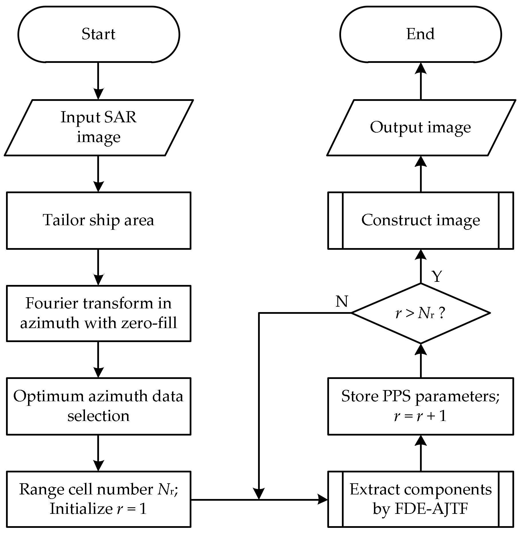
The imaging procedure of the SAR–ISAR hybrid method based on FDE–AJTF is shown in Figure 1.
The detail procedure is as follows,
- (a)
- Input a complex SAR image;
- (b)
- Tailor an effective area on the whole SAR image, in which the ship target is contained;
- (c)
- Translate the sub-image data to Doppler domain with zero-fill by Fourier transform in azimuthal direction;
- (d)
- Select the optimum azimuth data with the method in the Section 2.1;
- (e)
- Estimate the parameters and extract the components of all range cells by FDE-AJTF decomposition method as described in Section 2.2;
- (f)
- Construct the RID image at a certain time as described in Section 2.3.
- (g)
- Output the image.
For this procedure, the specific steps of FDE–AJTF to estimate the parameters and extract the components in a range cell were described in Section 2.2, and the steps of image construction were described in Section 2.3. Therefore, the two modules are not expanded in detail.
4. Simulation and Experimental Test
The feasibility and effectiveness of this proposed imaging method were verified by simulation and experimental test.
4.1. Simulation Test
A simulated moving ship imaging system for spaceborne SAR was built at first [2]. The scattering point model and imaging results are shown in Figure 2a–c.
As shown in Figure 2a,b, a nine-point model was adopted for the simulation. The imaging result without motion, in which the sub image of each point was similar to the others, is clear. In Figure 2c, the imaging result with motion is fuzzy and unfocused, and the scattering point images differ from each other. Because of rotation, the motions of every point were different. The exception is the central point, or the rotation center, which was well imaged because it was not influenced by rotational motion.
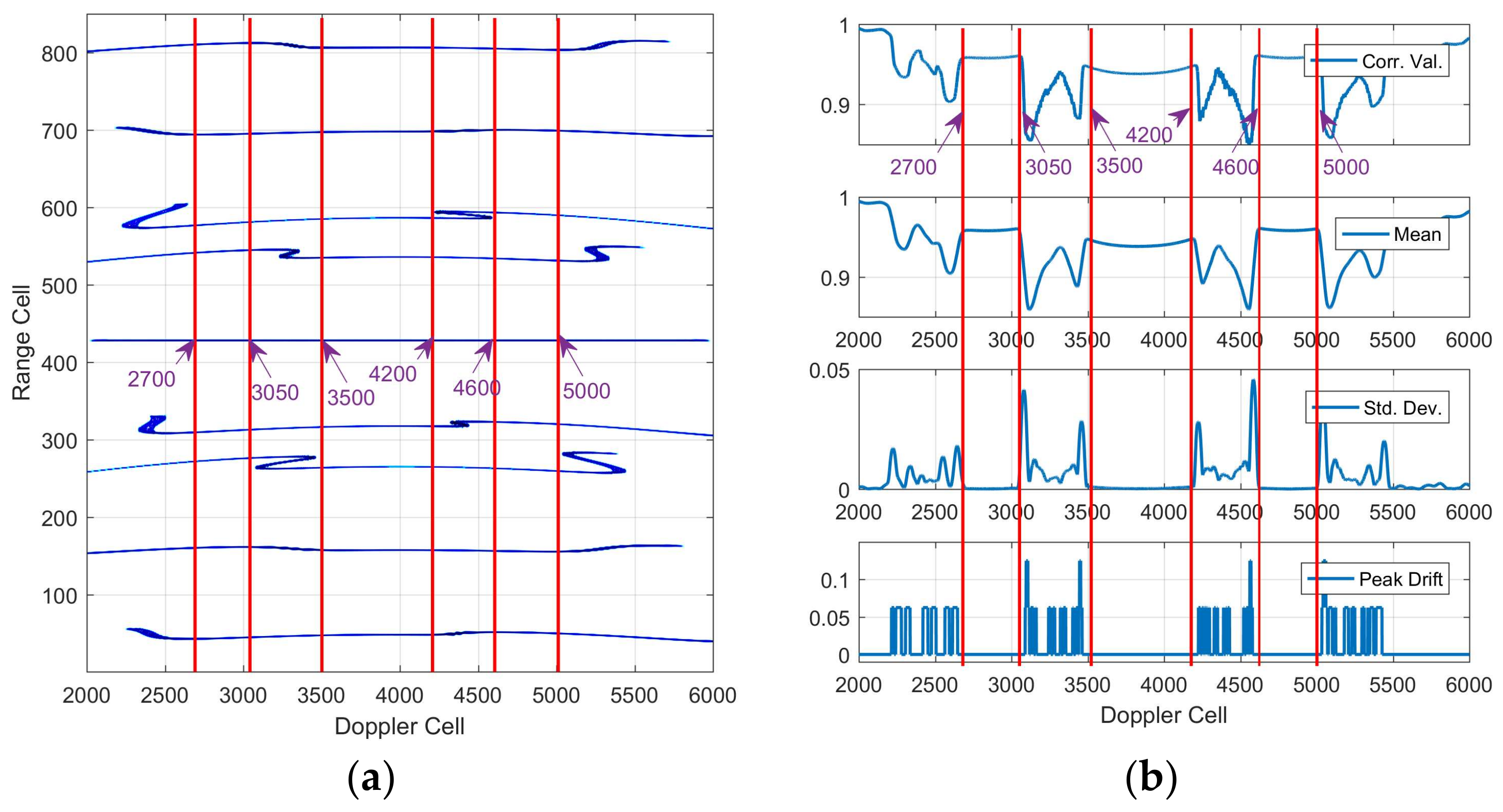
We translated the simulation data shown in Figure 2c to the range-Doppler domain with zero filling and calculated the four correlation characteristics. The results are shown in Figure 3.
As shown in Figure 3a, the envelope of each point migrated severely and differed from the other points, with even abrupt changes occurring in them. It is a difficult to align the whole envelopes correctly. Alignment is almost impossible when the near scattering points influence each other. As shown in Figure 3b, the four correlation characteristics reflected the conditions of envelope alignment at different sections, with the data performing well in sections [2700–3050], [3500–4200], and [4600–5000]. This result is intuitively in accordance accords with the changes shown in Figure 3a. Thus, these three sections may be chosen for the imaging process to improve the image effect.
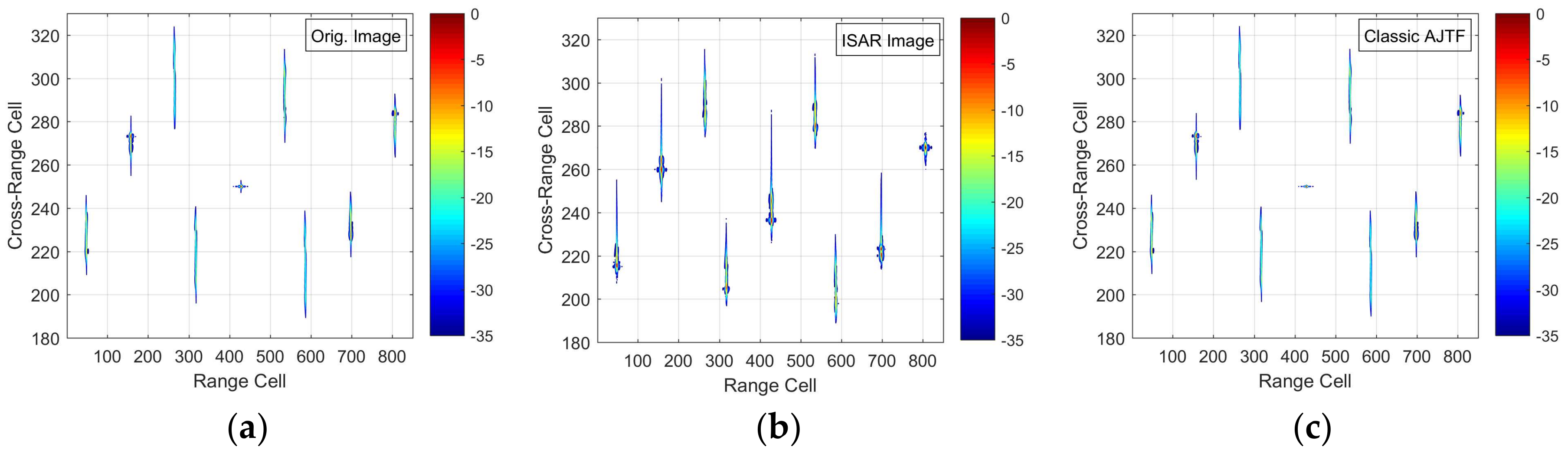
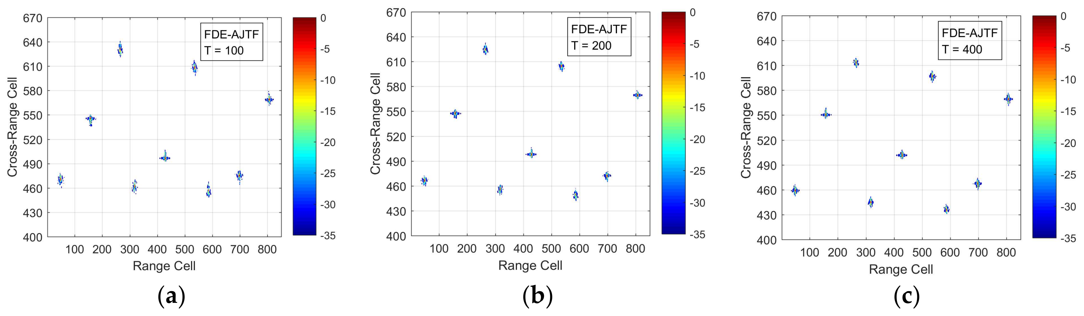
In accordance with the results shown in Figure 3, section [3601–4100] of the simulated data was selected for imaging. The data length was 500, and the number of side lobes was set at . The results using the classical methods of direct imaging, ISAR, and AJTF are shown in Figure 4a–c, while the results using the FDE–AJTF method at different times are shown in Figure 5a–c.
In Figure 4a, it is evident that slight fuzziness was reduced by imaging directly after selecting the optimum azimuth data; nevertheless, azimuth resolution was influenced by the time window and uncompensated complex phase. In Figure 4b, we see that the classical ISAR method could not improve the imaging effect. Instead, the central point was affected. The reason for this is that the well-aligned envelope migrated, creating an error in the aligning process because of the different migrations of the envelopes. As seen in Figure 4c, the classical AJTF method also showed no improvement, because this method could not compensate for the phase errors caused by three-dimensional motion.
In contrast, the results of the FDE–AJTF imaging method, shown in Figure 5a–c, are obviously superior, and much better than the results in Figure 4a–c. The distribution of the nine scattering points was varied with the azimuth time, which reflected the posture changes of the target, and this was another advantage of RID imaging method.
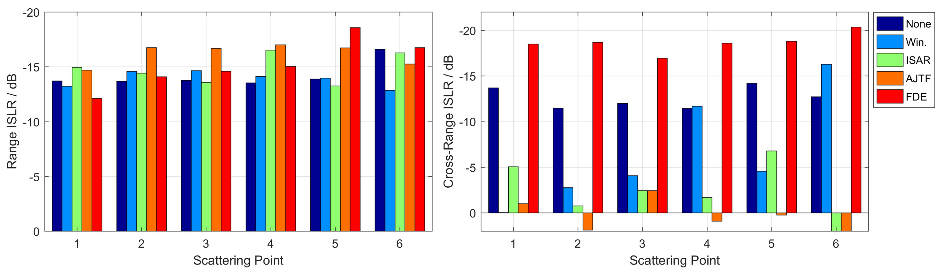
To compare the imaging effects of these imaging methods, the peak side lobe ratio (PSLR) and the integral side lobe ratio (ISLR) of the first six imaging points of each image were calculated and are shown in Figure 6 and Figure 7. These methods included imaging with no motion, as shown in Figure 2b; direct imaging after the windowing, classical ISAR, and classical AJTF methods, as shown in Figure 4a–c; and imaging via FDE–AJTF at T = 200, as shown in Figure 5b.
As can be seen in Figure 6 and Figure 7, the PSLRs and ISARs of the different images did not have many differences in range dimension, whereas those in the azimuth dimension differed strongly. It is clear that the azimuth imaging process was more influenced by the ship’s motions than by the range dimension. The azimuth PSLRs using FDE–AJTF imaging, as shown in Figure 6, were better than seen in the other three methods, approximately as good as those for the PSLRs with no motion. As shown in Figure 7, the ISLRs by FDE–AJTF were better than the others as well; better even than the ISLRs with no motion, owing to side lobe suppression in the image construction by the function, in accordance with Equation (8).
As shown in Figure 6 and Figure 7, the imaging effects were improved by the FDE–AJTF-based imaging method. The PSLR was increased more than 8 dB and the ISLR was reduced more than 12 dB under this simulation. Of course, in the experimental test, PSLR and ISLR cannot improve as much due to the influences of the scattering points near each other. On the other hand, PSLR and ISLR could not be measured accurately in the experimental test.
4.2. Experimental Test
The spaceborne SAR image of a moving ship from the experimental test is shown in Figure 8.
In Figure 8, it is evident that the ship image is severely fuzzy and unfocused, and few obvious scattering points could be distinguished effectively. The causes of this fuzziness are the complex phases and envelope migrations caused by the ship’s motion.
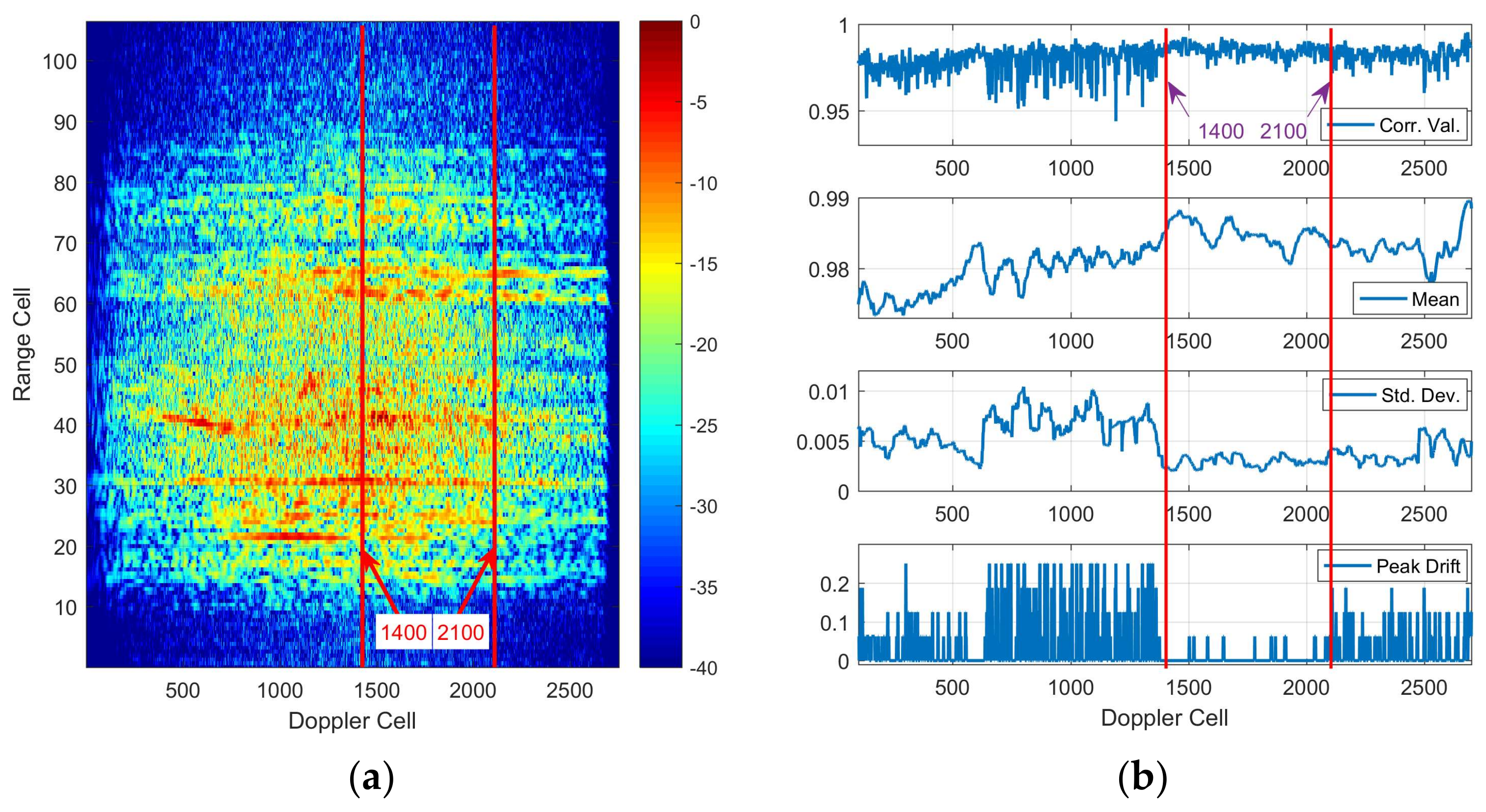
We translated the experimental data shown in Figure 3 to the range-Doppler domain with zero filling and calculated the four correlation characteristics. The results are shown in Figure 9.
The data in the range-Doppler domain was translated with zero fill, shown in Figure 9a; the envelopes also migrated differently in the different azimuth cells. As seen in Figure 9b, section [1400~2100] performed well in the envelope alignment, and can therefore be used for imaging in the latter process.
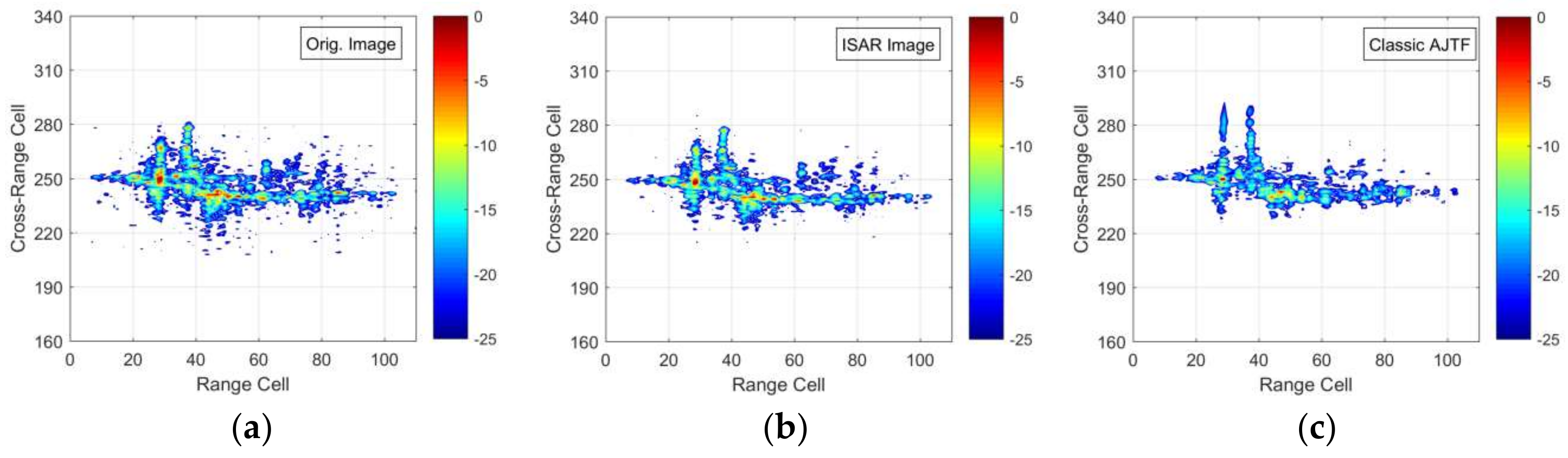
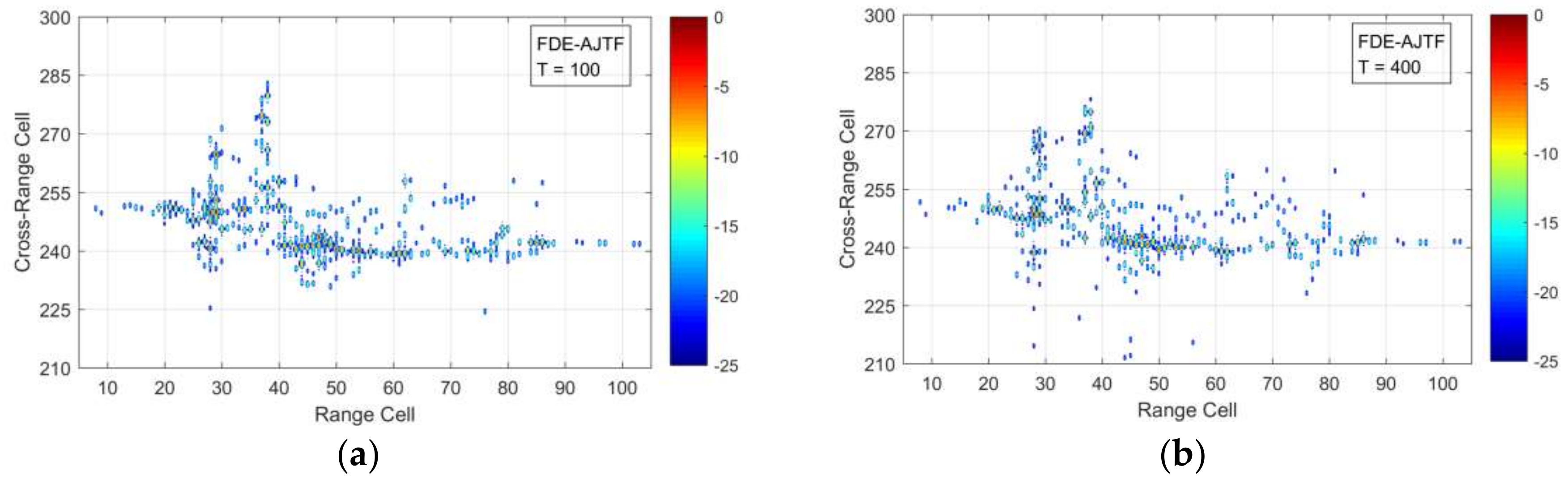
From the results of the experimental test shown in Figure 9, section [1501–2000] was selected for processing. The data length was 500, and the number of side lobes was set to . The imaging results obtained by the classical and FDE–AJTF imaging methods are shown in Figure 10a,b and Figure 11a,b.
As shown in Figure 10, the imaging effects using classical ISAR and AJTF were not improved, with few changes compared to the original image. In contrast, in Figure 11, the scattering points were extracted from every cell range by the FDE–AJTF imaging method. Image resolution was increased, more inner details were displayed, and the basic outline was maintained.
As shown in the imaging results of the simulation and experimental test, the image effects of ship targets were improved obviously by the proposed SAR-ISAR hybrid method based on the FDE-AJTF decomposition method. The performances of the proposed FDE-AJTF based imaging method were much better than the classic imaging methods such as the classic ISAR method and classic AJTF method, etc. by the comparisons between them. The feasibility and effectiveness of this proposed FDE–AJTF imaging method are, therefore, verified by simulations and experiments.
5. Conclusions
Ships are important types of ocean targets and have specific motion features caused by winds and waves. When imaged by high-resolution spaceborne SAR, however, these complex three-axis motions have a series of adverse effects, leading to fuzzy and unfocused imaging results. To address these problems, we propose a novel SAR–ISAR hybrid imaging method based on the FDE–AJTF decomposition method. This paper had four main parts. First, according to the correlation characteristics between every two adjacent range cells, a selecting method for optimum azimuth data was presented to reduce the influence of envelope migrations. Second, the FDE–AJTF decomposition method, which can estimate and extract the components in the echo signals, was presented. Third, an image construction method was proposed to reduce computation demands, allowing the display resolution and scale to be easily controlled. Finally, simulation and experimental tests were used to show and compare the imaging effects of different methods, verifying the feasibility and effectiveness of the proposed imaging method.
Acknowledgments
The authors are grateful for the financial support received from the State 863 Project of China (no. 2014AA7113016) and the Research Project of the State Key Laboratory of Complex Electromagnetic Environment Effects on Electronics and Information Systems (no. 2017Z0203B).
Author Contributions
Guochao Lao and Canbin Yin conceived and designed the method; Wei Ye guided the students to complete the research; Yang Sun, Guojing Li and Long Han performed the simulation and experiment tests; and Guochao Lao wrote the paper.
Conflicts of Interest
The authors declare no conflict of interest.
References
- Chen, V.C.; Li, F.; Ho, S.S.; Wechsler, H. Micro-Doppler effect in radar: Phenomenon, model, and simulation study. IEEE Trans. Aerosp. Electron. Syst. 2006, 42, 2–21. [Google Scholar] [CrossRef]
- Lao, G.; Liu, G.; Wu, X. The modeling and simulation of spaceborne SAR moving vessel imaging based on Matlab class. In International Conference on Frontiers of Manufacturing Science and Measuring Technology (FMSMT), Taiyuan, China, 24–25 June 2017; Atlantis Press: Paris, France, 2017; Volume 130, pp. 1583–1586. ISBN 978-94-6252-331-9. [Google Scholar]
- Xu, J.; Huang, Z.; Yan, L.; Zhou, X.; Zhang, F.; Long, T. SAR ground moving target indication based on relative residue of DPCA processing. Sensors 2016, 16, 1676. [Google Scholar] [CrossRef] [PubMed]
- Shen, M.; Yu, J.; Wu, D.; Zhu, D. An efficient adaptive angle-Doppler compensation approach for non-sidelooking airborne radar STAP. Sensors 2015, 15, 13121–13131. [Google Scholar] [CrossRef] [PubMed]
- Lombardini, F.; Bordoni, F.; Gini, F.; Verrazzani, L. Multibaseline ATI-SAR for robust ocean surface velocity estimation. IEEE Trans. Aerosp. Electron. Syst. 2004, 40, 417–433. [Google Scholar] [CrossRef]
- Phillips, L.C.; Turpin, T.M. Moving-target SAR/ISAR imaging using the ImSyn processor. Int. Soc. Opt. Eng. 1996, 2751, 219–229. [Google Scholar]
- Pastina, D. Rotation motion estimation for high resolution ISAR and hybrid SAR/ISAR target imaging. In Proceedings of the 2008 IEEE Radar Conference, Adelaide, Australia, 2–5 September 2008; pp. 1–6. [Google Scholar]
- Sun, C.; Wang, B.; Fang, Y.; Yang, K.; Song, Z. High-resolution ISAR imaging of maneuvering targets based on sparse reconstruction. Signal Process. 2015, 108, 535–548. [Google Scholar] [CrossRef]
- Martorella, M.; Acito, N.; Berizzi, F. Statistical CLEAN Technique for ISAR Imaging. IEEE Trans. Geosci. Remote Sens. 2007, 45, 3552–3560. [Google Scholar] [CrossRef]
- Pham, D.S.; Zoubir, A.M. Analysis of multicomponent polynomial phase signals. IEEE Trans. Signal Process. 2007, 55, 56–65. [Google Scholar] [CrossRef]
- Friedlander, B.; Francos, J.M. Estimation of amplitude and phase parameters of multicomponent signals. IEEE Trans. Signal Process. 1995, 43, 917–926. [Google Scholar] [CrossRef]
- Djurovic, I.; Stankovic, L. Quasi maximum likelihood estimator of polynomial phase signals. IET Signal Process. 2014, 13, 347–359. [Google Scholar] [CrossRef]
- Djurovic, I.; Simeunovic, M. Review of the quasi-maximum likelihood estimator for polynomial phase signals. IET Signal Process. 2018, 72, 59–74. [Google Scholar] [CrossRef]
- Peleg, S.; Porat, B. Estimation and classification of polynomial-phase signals. IEEE Trans. Inf. Theory 1991, 37, 422–430. [Google Scholar] [CrossRef]
- Wang, Y.; Abdelkader, A.C.; Zhao, B.; Wang, J. ISAR imaging of maneuvering targets based on the modified discrete polynomial-phase transform. Sensors 2015, 15, 22401–22418. [Google Scholar] [CrossRef] [PubMed]
- Jing, F.; Si, W.; Jiao, S. A hybrid LVD-HAF method of quadratic frequency-modulated signals. In Proceedings of the Applied Computational Electromagnetics Society Symposium—Italy (ACES), Florence, Italy, 26–30 March 2017. [Google Scholar]
- Zheng, J.; Su, T.; Zhu, W.; Zhang, L.; Liu, Z.; Liu, Q. ISAR imaging of nonuniformly rotating target based on a fast parameter estimation algorithm of cubic phase signal. IEEE Trans. Geosci. Remote Sens. 2015, 53, 4727–4740. [Google Scholar] [CrossRef]
- Popovica, V.; Djurovica, I.; Stankovica, L.; Thayaparanb, T.; Dakovica, M. Autofocusing of SAR images based on parameters estimated from the PHAF. Signal Process. 2010, 90, 1382–1391. [Google Scholar] [CrossRef]
- Kulkarni, R.; Rastogi, P. Multiple phase estimation in digital holographic interferometry using product cubic phase function. Opt. Lasers Eng. 2013, 51, 1168–1172. [Google Scholar] [CrossRef]
- Djurovic, I.; Simeunovic, M.; Wang, P. Cubic Phase Function: A Simple Solution to Polynomial Phase Signal Analysis. Signal Process. 2017, 135, 48–66. [Google Scholar] [CrossRef]
- Trintinalia, L.; Ling, H. Joint time-frequency ISAR using adaptive processing. IEEE Trans. Antennas Propag. 1997, 45, 221–227. [Google Scholar] [CrossRef]
- Yang, G.; He, Z. Improvement for ISAR Imaging Algorithms of Ship Targets. Mod. Def. Technol. 2013, 1, 47–52. [Google Scholar] [CrossRef]
- Thayaparan, T.; Brinkman, W.; Lampropoulos, G. Inverse synthetic aperture radar image focusing using fast adaptive joint time-frequency and three-dimensional motion detection on experimental radar data. IET Signal Process. 2010, 4, 382–394. [Google Scholar] [CrossRef]
- Lao, G.; Yin, C.; Ye, W.; Sun, Y.; Li, G. A frequency domain extraction based adaptive joint time frequency decomposition method of maneuvering target radar echo. Remote Sens. 2018, 10, 266. [Google Scholar] [CrossRef]
- Hu, G. Digital Signal Processing, 3rd ed.; Tsinghua University Press: Beijing, China, 2015; pp. 33–38, 135–140. ISBN 978-7-302-29757-4. [Google Scholar]
- Brinkman, W.; Thayaparan, T. Focusing inverse synthetic aperture radar images with higher-order motion error using the adaptive joint-time-frequency algorithm optimised with the genetic algorithm and the particle swarm optimisation algorithm-comparison and results. IET Signal Process. 2010, 4, 329–342. [Google Scholar] [CrossRef]
- Hassan, R.; Cohanim, B.; Weck, O.D.; Venter, G. A comparison of particle swarm optimization and the genetic algorithm. In Proceedings of the AIAA/ASME/ASCE/AHS/ASC Structures, Structural Dynamics & Materials Conference, Austin, TX, USA, 18–21 April 2005. [Google Scholar]
- Dorigo, M.; Stutzle, T. Ant Colony Optimization; Simplified Chinese Translation Edition; Tsinghua University Press: Beijing, China, 2007; pp. 65–68. ISBN 978-7-302-13887-7. [Google Scholar]
- Richards, M.A. Fundamentals of Radar Signal Processing, simplified Chinese translation ed.; Publishing House of Electronics Industry: Beijing, China, 2008; pp. 260–268. ISBN 978-7-121-06896-6. [Google Scholar]
Figure 1.
Imaging procedure.

Figure 2.
Scattering point model and imaging result of the simulation. (a) Scattering point model; (b) imaging result without motion; and (c) imaging result with motion.
Figure 2.
Scattering point model and imaging result of the simulation. (a) Scattering point model; (b) imaging result without motion; and (c) imaging result with motion.
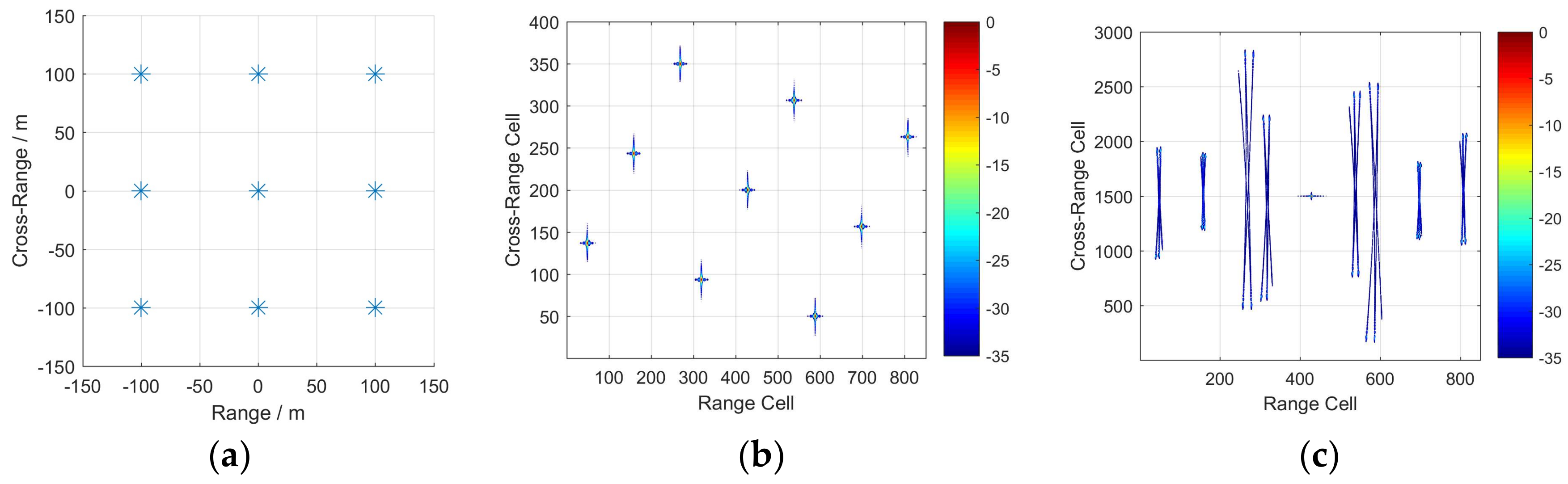
Figure 3.
Correlation characteristics of simulated data. (a) Data in the range-Doppler domain; and (b) the four correlation characteristics.
Figure 3.
Correlation characteristics of simulated data. (a) Data in the range-Doppler domain; and (b) the four correlation characteristics.

Figure 4.
Imaging results using classical methods. (a) Direct imaging; (b) classical ISAR; and (c) classical AJTF.
Figure 4.
Imaging results using classical methods. (a) Direct imaging; (b) classical ISAR; and (c) classical AJTF.

Figure 5.
Imaging results by FDE–AJTF method. (a) T = 100; (b) T = 200; and (c) T = 400.

Figure 6.
PSLRs in the range and azimuth dimension.
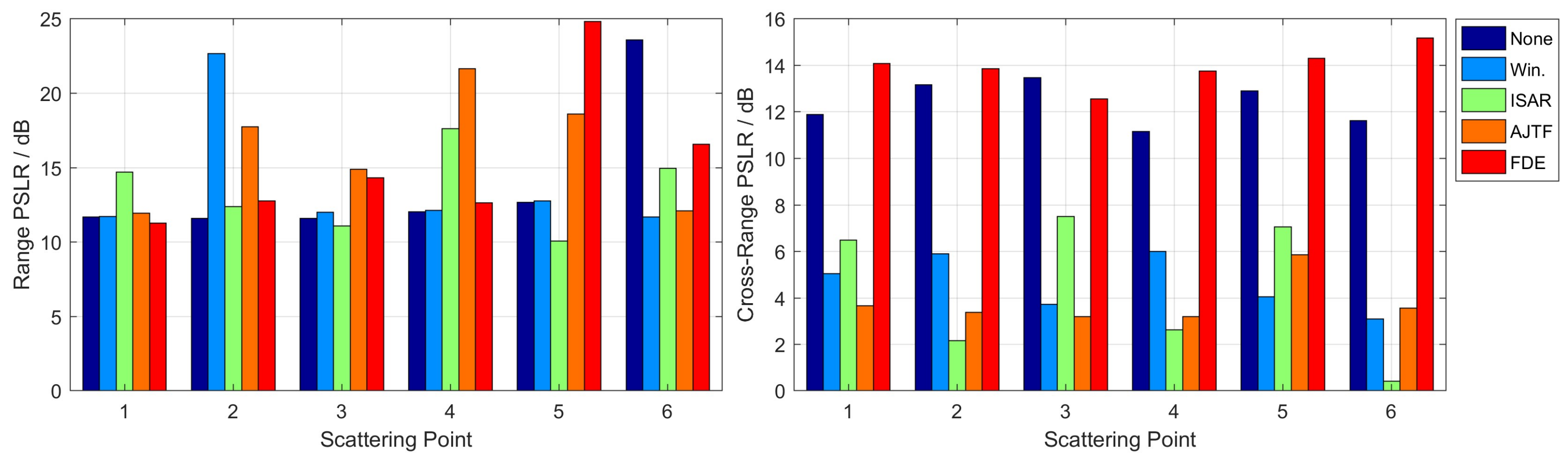
Figure 7.
ISLRs in the range and azimuth dimensions.

Figure 8.
A moving ship image via spaceborne SAR.
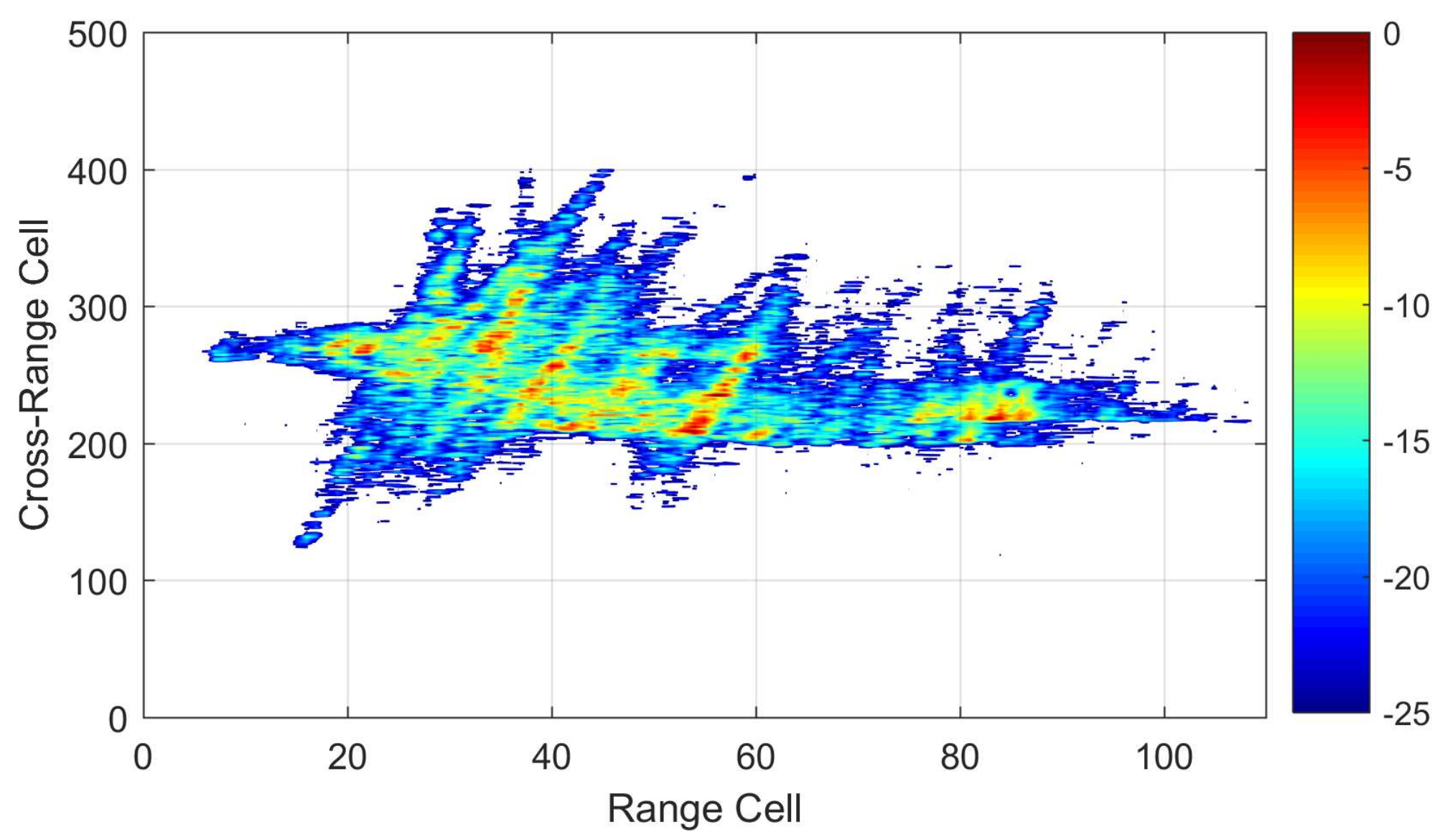
Figure 9.
Correlation characteristics of experimental test. (a) Data in range-Doppler domain; and (b) four correlation characteristics.
Figure 9.
Correlation characteristics of experimental test. (a) Data in range-Doppler domain; and (b) four correlation characteristics.

Figure 10.
Imaging results by classical methods. (a) Direct imaging; (b) classical ISAR; and (c) classical AJTF.
Figure 10.
Imaging results by classical methods. (a) Direct imaging; (b) classical ISAR; and (c) classical AJTF.

Figure 11.
Imaging results using FDE–AJTF. (a) T = 100; and (b) T = 400.

© 2018 by the authors. Licensee MDPI, Basel, Switzerland. This article is an open access article distributed under the terms and conditions of the Creative Commons Attribution (CC BY) license (http://creativecommons.org/licenses/by/4.0/).
Share and Cite
MDPI and ACS Style
Lao, G.; Yin, C.; Ye, W.; Sun, Y.; Li, G.; Han, L. An SAR-ISAR Hybrid Imaging Method for Ship Targets Based on FDE-AJTF Decomposition. Electronics 2018, 7, 46. https://doi.org/10.3390/electronics7040046
AMA Style
Lao G, Yin C, Ye W, Sun Y, Li G, Han L. An SAR-ISAR Hybrid Imaging Method for Ship Targets Based on FDE-AJTF Decomposition. Electronics. 2018; 7(4):46. https://doi.org/10.3390/electronics7040046
Chicago/Turabian StyleLao, Guochao, Canbin Yin, Wei Ye, Yang Sun, Guojing Li, and Long Han. 2018. "An SAR-ISAR Hybrid Imaging Method for Ship Targets Based on FDE-AJTF Decomposition" Electronics 7, no. 4: 46. https://doi.org/10.3390/electronics7040046
Note that from the first issue of 2016, this journal uses article numbers instead of page numbers. See further details here.