Study on Consulting Air Combat Simulation of Cluster UAV Based on Mixed Parallel Computing Framework of Graphics Processing Unit

Department of Mechanical and Aerospace Engineering, Chung Cheng Institute of Technology, National Defense University, Taoyuan 33551, Taiwan
Electronics 2018, 7(9), 160; https://doi.org/10.3390/electronics7090160
Submission received: 7 August 2018
/
Revised: 15 August 2018
/
Accepted: 20 August 2018
/
Published: 23 August 2018
(This article belongs to the Special Issue Selected Papers from the IEEE ICASI 2018)
Abstract
:This paper combines matrix game theory with negotiating theory and uses U-solution to study the framework of the consulting air combat of UAV cluster. The processes to determine the optimal strategy in this paper follow three points: first, the UAV cluster are grouped into fleets; second, the best paring for the joint operations of the fleet member with the enemy fleet members are calculated; thirdly, consultations within the fleet are conducted to discuss the problems of optimal tactic, roles of main/assistance, and situational assessment within the fleet. In order to improve the computing efficiency of the framework, this article explores the use of the NVIDIA graphics processor programmed through MATLAB mixed C++/CUDA toolkit to accelerate the calculations of equations of motion of unmanned aerial vehicles, the prediction of superiority values and U values, computations of consultation, the evaluation of situational assessment and the optimal strategies. The effectiveness evaluation of GPGPU and CPU can be observed by the simulation results. When the number of team air combat is small, the CPU alone has better efficiency; however, when the number of air combat clusters exceeds 6 to 6, the architecture presented in this article can provide higher performance improvements and run faster than optimized CPU-only code.
1. Introduction
In the 2017 Super Bowl midfielder show, Intel used 300 Intel drones to create a volleyball light show, and issued colorful lights, changed formations, and produced various patterns to employ drones besides aerial shooting or investigation, but also ‘performance’. It can be seen that the drone cluster technology will be the next development focus. Therefore, unmanned combat aircraft are expected to assist human pilots or perform autonomous air operations. Therefore, intelligent decision-making air combat maneuvering has always been a research hotspot. The matrix game [1] is the first proposed approach to solve the pursuer–evader game. Although the game-matrix approach is feasible as a maneuvering decision method, the solution of this method is only a suboptimal strategy sequence that satisfies the segmentation. In addition, the method is computationally intensive, especially when the maneuvering sets are complicated, the prediction time is long and makes the task difficult for the onboard computer to complete. The expert system [2] is also one of the traditional methods of intelligent air combat maneuver decision-making, but it can only be used to solve known problems. When encountering unknown problems, it still needs personnel participation rather than completely independent decision-making. Based on the influence diagram (ID), the research on the one-on-one air combat model can be referred to [3,4]. The literature [5,6] further proposes the ID improvement model of multi-aircraft cooperative air combat maneuver decisions. The combination auction theory is used to control the decision of multiple fighters to cooperate in close air combat, which can be seen in [7].
At present, air combat research mainly uses traditional artificial intelligence optimization theories and algorithms to calculate air combat decision sequences in a relatively fixed environment. For example, Ref. [8] proposed a genetic algorithm for interval grey simulated annealing to improve global search capabilities. A novel particle swarm optimization algorithm based on an adaptive stochastic learning method was proposed [9] to find an optimization function with fewer parameters. In [10], a predictive fuzzy inference system is proposed as a smart maneuvering decision system, which simulates the human thinking ability and the maximum energy of the virtual aircraft as the air combat decision. In recent years, the successful application of machine learning technology in many fields has provided new ideas for the study of intelligent air combat decision-making. It is an effective method of applying reinforcement learning (RL) in the field of air combat, because it can interact with the environment through repeated experiments and obtain optimal strategies through iteration [11]. However, due to the computational overload caused by the curse of dimensionality, the traditional RL method is not suitable for solving large-scale Markov decision processes (MDP) such as air combat. In [12,13], an approximate learning method combining approximation techniques with reinforcement learning is used to approximate a value function or a state space by a function approximator. Avoiding accurate solutions can alleviate the problems caused by the dimensional curse to a certain extent. Ref. [14] refers to some typical studies using Atari games and AlphaGo [15,16] using deep learning and reinforcement learning, and conceived the application of this method to air combat decision-making by using a multi-layer stacking deep neural network (DNN) as a function approximator. Because of its robust and accurate capacity, it can accurately represent complex state spaces and use the lessons learned as the highest reward option to get the system into a better state. In order to avoid relying on prior knowledge and good local optimality of exits, Ref. [17] uses Q learning in reinforcement learning algorithms for air combat target assignment. In [18], it is proposed to use neural networks in heuristic reinforcement learning to learn the process of the reinforcement learning to accumulate knowledge and stimulate the search process.
In the cluster confrontation, it is not only as simple as the dual air battle is considered to be a zero-sum game, in fact there is a cooperative and coordinated team-mate relationship between individuals in their own cluster. For example, the air combat between the two pursuers and a fugitive was established as a nonzero-sum differential game. Ref. [19] proposes the variation and Legendre pseudo-spectral methods to solve the nonzero-sum multi-player Nash differential game. Ref. [20] considered the mixed strategy Nash equilibrium (MSNE) with n-person and n-strategies. In air combat, the target-defender team strives to maximize the terminal separation of the target from the attacker, while the attacker sought to minimize the separation. Ref. [21] proposed a differential game approach to derive the optimal strategies for the three agent. As the team-mates’ survivability increases and the overall threat to the enemy intensifies, there should be cooperation and coordination among individual clusters in the drone cluster confrontation. Therefore, Ref. [22] introduces the fusion mechanism of differential game and negotiating theory. Ref. [23] addressed a zero-sum matrix game problem of evasion from multiple pursuers by reducing it to a multi-act, two player zero-sum game.
In the confrontation game, both offensive and defensive players need to consider the impact of threat assessment, economic strategic value assessment, and overall system task payment. Therefore, a multi-objective optimization corresponding performance evaluation model is proposed, and the decision-making problem of multi-target cooperative attack is transformed into missile attack-matching optimization problem. Therefore, the issue of weapons target assignment (WTA) is crucial to the strategic planning of military decision-making operations. It defines the best way to allocate defensive resources for defense threats in combat scenarios. However, the process of air combat is dynamic and therefore contains many uncertainties. It is thus difficult to obtain a decision sequence that conforms to the actual situation of air combat using traditional theoretical methods. The self-optimization and self-organization of tactical re-planning in real time must overcome the dynamic changes in the number and location of nodes in the combat process in order to maximize the expected return and effectively solve the multi-fighter cooperation strategy. However, in the uncertain case, multi-objective optimization is difficult to solve the WTA problem. Ref. [24] proposed a hybrid fuzzy multi-objective programming and multi-objective quantum behavior particle swarm optimization algorithm to overcome this problem. Ref. [25] proposed an interval-intuitive fuzzy Petri net to define the degree of membership in air combat.
Due to oversimplified assumptions, heavy computational load and limited scalability, previous studies on air combat often have limitations. As the number of control points and the number of drones increase, so does the complexity of the problem. Therefore, the biggest bottleneck encountered in the research of cluster cooperative air combat simulation is that the calculation speed cannot reach real-time. The advent of more unmanned aerial vehicles for team air combat simulations demands a commensurate growth in computational power. In addition, if there is external warfare in the line of sight, it needs to combine radar and missile theory. Complex and huge calculations will cause delays in simulation, and it is impossible to immediately make the best strategy to counter enemy attacks. Therefore, how to accelerate computational efficiency has become a key technology, and computational parallelism seems to be the most successful method at present. In recent years, parallel computing on the general-purpose computing on graphics processing unit (GPGPU) using the CUDA architecture has been widely used. GPGPU provides a vast number of simple, data-parallel, deeply multithreaded cores and high memory bandwidths at very low cost, which has recently attracted the attention of many application developers as commodity data parallel coprocessors. For example, Ref. [26] introduced Hough transform, Kalman filter, and clustering with GPUs for fast multi-line tracking for vision based intelligent vehicle. A genetic algorithm working in concert with a clustering algorithm is used by [27] to quickly compute the desired routes and GPU is used in this work to enhance the computational execution rate. Ref. [28] applied the K-means and parallel genetic algorithm on CUDA architecture to search a solution to the problem of minimum time coverage of ground areas using a number of UAVs. The GPU also exhibits excellent properties in computational fluid dynamics—e.g., Ref. [29] described the most advanced results of fluid dynamic simulations of high-enthalpy flows and used MPI-CUDA approach to overcome the huge computational cost. Ref. [30] present an implementation of the spectral-element method for simulation of two-dimensional elastic wave propagation in fully heterogeneous media performed on a GPU cluster. In the biophysical model field, Ref. [31] explored the application of GPU to simulate of cardiac bioelectric phenomena. Ref. [32] demonstrates the outstanding performance of CUDA in image processing research by several classical image processing algorithms. The results of the literature show that the GPGPU processing data volume and calculation speed are far greater than the CPU.
2. Related Work
This article is different from [19,20,21,22] using differential game as the decision core but combines the matrix game with the negotiation theory and uses the U-solution to study the theoretical framework of the cooperative air combat. The advantage of using matrix game is that when we calculate the best strategy, only Runge-Kutta method to integral the motion equations is necessary, avoiding the differential game demand solving the double side extreme value problem. Similarly, Ref. [23] also uses matrix games to consider the problem of multi-vehicle chase single vehicle, but its strategy of pursuit/evasion is based on the existing MATLAB package ‘cvx’ [33], and no specific recommendations are made on how to accelerate the calculation of the strategy as proposed in this paper.
In determining the optimal strategy of a cluster of UAVs, this paper follows these points: first, the UAV cluster are grouped into fleets, and second, the best paring for the joint operations of the fleet member with the enemy fleet members are calculated. Thirdly, consultations within the fleet are conducted to discuss the problems of optimal tactic, roles of main/assistance, and situational assessment within the fleet. Ref. [34] also mentioned the concept of grouping multi-fighter cooperative air combat into small teams similar to this paper, but [34] adopting multi-stage influence diagrams to calculate the best strategy, which is not the same as using matrix game in this article. There is also no mention of how to speed up the calculation load. In addition, the target of chasing after locking is not related to missile attack-matching optimization problem in this paper. For the missile attack matching optimization (WTA) problem, please refer to [24,25]; for further exploration of effective range, please refer to [35,36].
On the other hand, to speed up the computational speed of UAV cluster negotiating air combat and expect to overcome the problem of huge computational delays as the number of clusters increases, C++ should be a good candidate because it can run on different CPUs or cores by allowing code to run in parallel and allowing code to run asynchronously instead of serially to improve performance. On the other hand, MATLAB’s advanced programming syntax and user-friendly environment make it ideal for writing technical code. However, MATLAB does not allow code to be executed on different CPUs or cores but uses the interpreter enabling of running code asynchronously, which slows down processing, especially when executing loops extensively. However, using NVIDIA’s CUDA-enabled GPUs to execute multiple threads is currently the hottest technology. Using CUDA, all the pipeline stages can be combined to execute a number of operations simultaneously. Ref. [37] discusses the principles and methods of hybrid programming, where MATLAB integrates with other languages such as Visual C++. The results show that mixed programming with different tasks can be achieved by compiling different MATLAB programs, making the necessary settings and replacing the corresponding C++ code. However, if one wants to use multi-core processors, GPUs, and clusters of computers to solve computational and data-intensive problems on MATLAB, one must use the Parallel Computing Toolbox and the Distributed Computing Server. Hence, this paper wants to try to use C++ to call CUDA for parallel computing and parallel for-loops without Parallel Computing Toolbox on MATLAB. This paper uses a mixed program of C++/CUDA and MATLAB to combine the advantages of C++/CUDA and MATLAB to form the multi-core and GPU parallel computing architecture of MATLAB/C++/CUDA, trying take full advantage of MATLAB’s programming flexibility by enhancing its performance. Some of how CUDA plays a potential role in accelerating MATLAB’s program execution is discussed in [38,39,40]. For example, [38] explores the potential benefits of integrating MATLAB with CUDA and describes a systematic approach to implementing vortex dynamics on CUDA. Another similar work is described in [39], which describes the benefits of integrating CUDA into MATLAB to accelerate its performance. The focus of this work is on the use of 2D wavelet transform for CUDA medical image compression. It first implements 2D-DWT in CUDA C and wraps it into a MEX file. Ref. [40] introduced a new method of achieving white balance using MATLAB and CUDA to achieve load balancing between CPU and GPU in a dynamic environment. By connecting MATLAB to CUDA and parallelizing the most time-consuming part of the MATLAB code white balance, the processing speed can be significantly faster. The methods presented in [39,40] are very similar to the proposed approach in this paper. In [39], CUDA function is only called on MATLAB, so it does not use MATLAB’s flexible programming structure. Although Ref. [40] introduced MATLAB to connect with CUDA and parallelize MATLAB code, the integration process is not as detailed in this article. As far as the author knows, the proposed architecture applied to accelerate the computation of air combat maneuver decision-making has not been proposed in any journals or conferences. Although the hardware device is old in this paper, the concept is the latest and interested readers can refer to the architecture of this article to test the effects on the latest GPUs.
3. Best Solution to Consulting Air Combat of Clusters
In one-on-one air combat, UAVs hope that they can grasp their advantages during the engagement process, form a threat to the enemy planes, or prevent the enemy planes from attacking the opponent. The competition between rivals is similar to the zero-sum game. Although, the basis of cluster air warfare is air-to-air combat, however, unlike one-on-one air combat, there is cooperation within the cluster group. Therefore, the team consulting air combat has two characteristics: (1) under the premise of improving the overall advantages, each UAV may separately or collectively attack the enemy aircraft; (2) when a friendly aircraft deters the threat of an enemy UAV, another UAV can ignore the threat that the enemy UAV poses to him and in turn launch a bold attack, making the strategies and maneuvers that cannot be or are not daunting during one-on-one combat to increase the kill rate. Under these two characteristics, the first step in determining the best strategy for cluster air warfare is to first divide the cluster into multiple fleets so that the cluster air warfare can be converted into fleet operations, and the advantages and weighting factors of air combat can be optimized by establishing fleets. It can improve their survivability and increase the threat and killing of enemy aircraft.
After dividing the air combat in a cluster into several small aircraft teams, we must then solve two problems: (1) how our team members are paired with the enemy fleet members; (2) the best strategy for both the enemy and me after the pairing. Therefore, this article will discuss the following aspects:
- The grouping principle of converting large-scale air combat into fleet operations;
- Optimize the target of fleet attack using negotiation theory;
- Optimize in-team marshalling by negotiation theory;
- The role of individuals in the fleet;
- Individual air combat within the fleet, using the game theory to find the best chase/escape strategy.
This paper introduces a method to optimize the overall attack benefit, called the utilitarian solution (abbreviated as U solution) algorithm, conducts the matching of rivals and friends, the calculation of weight values, and the prediction of the best strategy of both parties to determine the target of attack and the role played in the fleet, and the best strategy to increase overall attack effectiveness. Processes are as shown in Figure 1.
3.1. Cluster Air Combat Turned into Multiple Fleet Operations
The formation of the fleet is usually preceded by pre-operational mission cues that have been identified and rarely change in air combat unless special circumstances prevail. Therefore, this paper directly selects our k drones as a team, a total of m teams, denoted , I = 1~m; enemy aircraft will be divided into a team as the nearest each k, assuming there are n teams, denoted , j = 1~n. The centroid of each team represents the virtual aircraft of the team, so the problem is simplified to that of our m drones against n hostile aircraft. The centroid of the ith team () can be calculated by
This centroid is considered as a virtual UAV whose speed is obtained by vector addition.
The roll angle and the pitch angle of the virtual UAV are calculated by the following formula
We have divided the cluster air warfare into a small aircraft team. However, in the air combat, to solve the matching problem between our fleet and the enemy fleet, we must introduce negotiation theory and weight value calculations to determine the target of attack and the assigned role of each aircraft in the team. Take the air combat of two teams of two UAVs each as examples. The UAVs 1 and 2 score functions are and , respectively. We can set the score function as the total superiority value. The superiority values may include speed scoring, azimuth scoring, distance scoring, and altitude scoring [1,41]. If we set our score to be low, our overall best (superiority) U solution is
Equation (8) indicates that in the case where two UAVs choose the best match for the enemy fighter, the advantage score (the superscript “*”) sum is the lowest of all possible match combinations. The choice of and can be adjusted in different combat situations. Determine the weight values should be met: (1) is a function of the superiority value; (2) the emphasis on a certain fighter by increasing the weight value within the fleet; (3) when the overall fleet is in an advantage, the greater weight is assigned to the aircraft whose superiority value is better; otherwise, when the overall fleet is at a disadvantage, the aircraft with a worse advantage value has a greater weight value. It should be noted that the weights must be normalized so that the sum of all weights is 1. We adopt the weights usually in this paper as
According to the formula (8), it can be extended to m virtual aircrafts to n virtual enemy aircrafts (assuming m > n), and there are a total of probability superiority values. The best negotiation matchmaking team between the virtual aircraft fleets can be obtained to seek the best interests
where is determined as
where is still set as the total superiority of our ith virtual aircraft. The Equation (10) indicates that in the case where all aircraft fleets choose the best match for the enemy fighter fleets, the advantage score (the superscript “*”) sum is the lowest of all possible match combinations. Under the premise of the best overall advantage, multiple teams may attack the same team and each time interval determines whether it is necessary to re-determine the target.
3.2. Fleet Negotiation
As shown in Figure 1, the fleet air combat will be further divided into one-on-one air combat, using the negotiated theory and weight values again to determine the strategy of the two sides of aircrafts. If it is assumed that the decision within the team will affect each other, and each aircraft has seven strategies shown in Figure 2a. Define the seven strategies of our fighters as set and the seven strategies for enemy fighters as set .
Under each combination, the strategy combination of the two parties for m UAVs and n enemy UAVs can be expressed as following matrix
where represents the strategic pairing of the p-th row and the q-th column of the matrix. Referring to Figure 3, the current positions, attitudes and speeds of k our fighters (, i = 1~k) and k enemy fighters (, j = 1~k) are given. Figure 2b illustrates the fighter body axes with respect to the Earth and/or inertial reference axes. Referring to Figure 2b, under each strategy pairing, the equations of motion for solving an UAV is [42]
Symbols are described as follows: is flight path angle, the angle between UAV’s speed vector and horizontal plane; is azimuth angle, the angle between UAV’s speed vector project on horizontal plane and the X-axis; are the inertial coordinates; is UAV’s load factor along direction; is UAV’s load factor along -axis direction; is the rotational bank angle, which rotates around the heading direction. The acceleration commands (, , ) due to actuator dynamics are given by
where and are time constants of and , respectively; is natural frequency and is damping ratio, determined by the performance of UAV. The equations of motion (13) to (21) combine with transformation of coordinate will be able to predict UAV’s dynamics and position accurately, and the prediction superiority values including speed scoring, azimuth scoring, distance scoring, and altitude scoring can be evaluated. Let the superiority value of on enemy aircraft to is denoted by to under the strategy pairing , and the following mathematical symbols are defined.
The U value can be obtained under the strategy pairing as
Under all strategies pairing , a total of the matrix shown in Figure 3 needs to be completed. The best negotiation strategy between the aircraft team can be obtained to seek the best interests
where u is our UAV strategy, v is the enemy UAV strategy, the superscript “*” represents the best strategy, the subscript “*” indicates the most favorable of our attacking strategy, and no subscripts indicate other our attacking strategy. It is equivalent to finding the saddle point in the group combination to solve (25):
With the number of aircraft increasing, the strategy combination will form a huge matrix. At this time, the sequence calculation will not be able to make the reaction decisions of the team in real time. Therefore, as shown in Figure 3, this paper considers CUDA parallel computation to speed up the optimal solution of the strategy combination matrix.
The biggest difference between the matching with the fleet is the identification of the role of each fighter within its own fleet, including determining the dominant role and the main or assist attack role:
- (1)
- Offensive and assist roles in air combat: if the joint strikes, each UAV will play a different role in the combat group, and the better superiority value is (relatively dominant) the offensive UAV, and the rest will be an assistant. As the main attacker has a better value, the enemy has less chance of winning. In contrast, the enemy has a greater chance of winning again the assisting UAV which has a lower advantage. To make the superiority better, the enemy should compete against the assisting UAV to increase the advantage value with the best strategy. From our point of view, the assisting UAV at this time has deterred the threat of the enemy UAV. Therefore, the main attacker can ignore the threat which poses to him and use a single-player tactic to attack the enemy aircraft boldly. This is a dare to or impossible tactic during one-on-one air combat, which has increased the kill rate as a whole. The main attack and assist role are determined by in (22), the biggest one is the main attack, and the rest are assists. The strategy of the assisting machine uses (25) to find the best decision; while the remaining one is the main attacker, at this time, look for the strategy to minimize the value in (23). The flow chart for the role of the main attacker and assistant determined is shown in Figure 4.
- (2)
- Situational assessment: this is mainly determined by the superiority value of the UAV. If the superiority value is superior, then the role is the attacker, otherwise it is the evasion side. If the sum of the advantage values is required to be the largest, the UAVs will only focus on the attack. When the UAV is at a disadvantage and is possible shot down, the advantage value will be very small, and the unmanned aerial vehicle will not focus on the most threatening UAV but it will attack another UAV to increase its advantage value. This kind of unreasonable phenomenon needs to be corrected by judging the superiority value. The flow chart for situational assessment is shown in Figure 4. Assuming that now the superiority value for is at a disadvantage, should escape directly. If is on a very disadvantageous position, the other aircraft will help escape and pin down the enemy to increase ’s chances of escape.
4. Using MATLAB/CUDA to Accelerate the Best Solution
In the multiple air combat simulation, we mainly calculated the tactics of our military fleet (Blue Army) and enemy fleet (Red Army) and the trajectory between the two sides. The strategy and the trajectory are calculated based on the results obtained from the previous point in time. In this case, parallel computation cannot be used. Therefore, we use the decentralized operation for the Blue Army and the Red Army. The OpenMP is introduced to perform multi-core decentralized operation. Referring to Figure 5, we assign the calculations of the strategy and movement trajectory of the Blue Army and the Red Army to multiple CPU cores for calculation individually. The collaborative analysis and calculation of air combat between the Blue and Red Army can be performed at the same time.
However, the tactical judgments are more complex as the number of aircraft increases. Fortunately, CUDA technology provides computationally intensive applications with the processing power of the GPUs through a CUDA C programming interface. However, in fact, writing CUDA programs is not easy, and testing and modification is time consuming, so it is difficult to write a CUDA program for the entire multi-fighter air combat simulation. At present, even if there are APIs like CUBLAS and CUBLASXT to help linear algebra operations—such as vector multiplication, matrix multiplication vectors, matrix multiplication matrices, etc.—to help the simplicity and convenience of the entire program, writing CUDA programs is still not easy. Therefore, although the ideal multi-fighter air combat simulation is written in CUDA and the simulation efficiency should be greatly improved, but MATLAB is still a time-saving exercise if one wants to validate the design in a convenient and simple working environment. Although MATLAB is an easy to program development environment, the use of interpreter and memory latency issues can have a huge negative impact on performance. Many solutions to the MATLAB performance bottleneck have been proven in the relevant literature, one of which is the hybrid programming concept. By combining MATLAB with other languages such as C++, MATLAB’s programming flexibility is preserved, and the fast processing capabilities of other languages such as C++ are also utilized. The concept is to use CUDA parallelization and invoke it in the MATLAB environment by using the MEX function. In this way, different time-consuming parts of the MATLAB algorithm can be parallelized with CUDA and called in MATLAB. Therefore, for the goal of accelerating our approach by interfacing with CUDA and GPU, we must modify the script to MEX and CUDA cu files. By the way, there is another advantage to using the MEX function. The MEX function can not only transfer data between MEX files and MATLAB, but also call MATLAB functions in functions written in C, so MATLAB’s rich libraries are available in C.
Our work is done in two steps: the first step is to write a CUDA code of calculating the optimal strategy that performs the solutions of the equations of motion, the prediction of superiority values, U values evaluation and solves the matrix game in (25) that will be ported to CUDA, as mentioned the processes in Figure 3. The CUDA code is compiled via the NVCC compiler (NVCC is used to compile the CUDA code). After compilation, we can generate the .obj file. The second step is to write a C++ file to call the .obj file to package the CUDA architecture in the C++ language into MATLAB executable file. The MATLAB’s built-in instruction “mex” can be applied to wrap a C++ file including .obj files, CUDA header files, and function libraries to generate binary MEXw32 or MEXw64 file, which can be called in MATLAB as in any other MATLAB function. The mixed parallel computing framework of graphics processing unit is shown in Figure 5. In particular, the MATLAB code then runs in double precision mode and the data is converted to single precision before being transferred to the GPU. Therefore, the calculations on the GPU are executed as single precision arithmetic and the results are converted back to double precision before returning the results to MATLAB.
With reference to Figure 3, the position, attitude and speed data matrix of all the fighters of the Blue Army and the Red Army are transmitted to the GPU via the functions written in C++ to communicate MATLAB and CUDA. The strategy combination of the two armies for k Blue UAVs and k Red UAVs can be expressed as matrix according to (12). Each strategy combination uses a GPU’s thread to solve the motion equations of (13) to (21) in a time interval, and predicts the position, attitude, and velocity data of all the fighters of both fleets at the next time interval. This data is still calculated in the GPU’s thread for all fighters’ dominant values described in (22), and then all U values from (23) are calculated in parallel. Using the function written in CUDA to get the minimum or maximum value from the array satisfied (25) to find the best strategy for both side’s fighters. This strategy is passed back from the GPU back to MATLAB to continue the subsequent air combat simulation. After parallel calculations, when UAVs are locked by the radar, missiles are launched, and the missile guidance law is calculated by a CPU. For related missile guidance papers, please refer to [43].
In the above-mentioned best strategy of satisfying (25), it is necessary to first find the maximum value of each row in array (assuming the higher the enemy’s score is the better), and then find the minimum value in the maximum vector, and generate the corresponding strategy pairing. It is the best strategy for both our aircraft and the enemy. In the process, the CUDA parallelization method is used to find the maximum/minimum value of the vector. The concept is: first compare each two elements of the vector with each other, select a larger value, and then compare each of the two elements with the selected value. After comparison according to the above procedure, the maximum value of the vector can be selected. Because the comparison process is calculated in parallel, it can be much faster than the non-parallelization method. Because CUDA has more computational cores, a block can cover up to 512 threads, so we can perform large-value selection operations for each column at the same time. Taking 2 × 2 air combat as an example, first calculate the maximum value of each row in the U value matrix to obtain a column vector matrix; then compare the column vector with each other according to the above principle, and place the smaller one element on the first element of the column. After repeated comparisons, a minimum value can be obtained, which represents the minimum value of the Red Army’s maximum superiority value, and the maximum value of the Blue Army’s smallest superiority value. This is the saddle point of matrix. The program cumax.cu for finding the minimum value of CUDA is listed below. It is noted that the optimized library, such as CUBLAS, have not been used for the parallel implementation in our search.
In the below C++ program, the function g_kel is called mainly. Because many CUDA syntaxes are used, it is necessary to wrap it with extern “c”.
cumax.cu
extern “C” void g_kel(float* input, float &output, int &ind, int num );
#include <iostream>
using namespace std;
__device__ void cuMAX(float& a, float& b, int &c, int &d) {
  if (b>a) {
    a=b;
    c=d;  }}
__global__ void cuscanmax1(float* indata, float* outdata, int* index, int n) {
  int t=threadIdx.x;
  int b=blockIdx.x;
  int bdim=blockDim.x;
  int gdim=gridDim.x;
  int m=bdim*gdim;
  float stand = -99999999.0f;
   __shared__ float w[512];
  __shared__ int s[512];
  w[t] = stand;
  s[t] = 0;
  __syncthreads();
  for (int k=bdim*b+t; k<n; k+=m)
    cuMAX(w[t], indata[k], s[t], k);
  __syncthreads();
  if (t<256) cuMAX(w[t], w[t+256], s[t], s[t+256]);
  __syncthreads();
  if (t<128) cuMAX(w[t], w[t+128], s[t], s[t+128]);
   __syncthreads();
  if (t<64) cuMAX(w[t], w[t+64], s[t], s[t+64]);
  __syncthreads();
  if (t<32) cuMAX(w[t], w[t+32], s[t], s[t+32]);
  if (t<16) cuMAX(w[t], w[t+16], s[t], s[t+16]);
  if (t<8) cuMAX(w[t], w[t+8], s[t], s[t+8]);
  if (t<4) cuMAX(w[t], w[t+4], s[t], s[t+4]);
  if (t<2) cuMAX(w[t], w[t+2], s[t], s[t+2]);
  if (t<1) cuMAX(w[t], w[t+1], s[t], s[t+1]);
  __syncthreads();
  if (t==0) {
    outdata[b] = w[0];
    index[b] = s[0];  }}
__global__ void cuscanmax2(float* indata, float* outdata, int* index, int n) {
  int t=threadIdx.x;
   __syncthreads();
  if (t<256) cuMAX(indata[t], indata[t+256], index[t], index[t+256]);
  __syncthreads();
  if (t<128) cuMAX(indata[t], indata[t+128], index[t], index[t+128]);
   __syncthreads();
  if (t<64) cuMAX(indata[t], indata[t+64], index[t], index[t+64]);
  __syncthreads();
  if (t<32) cuMAX(indata[t], indata[t+32], index[t], index[t+32]);
  if (t<16) cuMAX(indata[t], indata[t+16], index[t], index[t+16]);
  if (t<8) cuMAX(indata[t], indata[t+8], index[t], index[t+8]);
  if (t<4) cuMAX(indata[t], indata[t+4], index[t], index[t+4]);
  if (t<2) cuMAX(indata[t], indata[t+2], index[t], index[t+2]);
  if (t<1) cuMAX(indata[t], indata[t+1], index[t], index[t+1]);
  __syncthreads();
  outdata[0] = indata[0];
}
void g_kel(float* input, float &output, int &ind, int num ) {

  float *cudainput, *cudaoutput;
  int *cudaindex;
  int sizedata = 4 * num;
  cudaMalloc((void**)&cudainput, sizedata);
  cudaMalloc((void**)&cudaoutput, 2048);
  cudaMalloc((void**)&cudaindex, 2048);
  cudaMemcpy(cudainput, input, sizedata, cudaMemcpyHostToDevice);

  cuscanmax1<<< 512, 512 >>>( cudainput, cudaoutput, cudaindex, num);
  cuscanmax2<<< 1, 512 >>>( cudaoutput, cudaoutput, cudaindex, 512);
  cudaMemcpy(&output, cudaoutput, 4, cudaMemcpyDeviceToHost);
  cudaMemcpy(&ind, cudaindex, 4, cudaMemcpyDeviceToHost);
  cudaFree(cudainput);
  cudaFree(cudaoutput);
  cudaFree(cudaindex);
}
In addition, the procedure for calling CUDA to find the best strategy in Figure 3 is also solved by the equations of motion (13) to (21). CUDA can also provide a fast computing platform for the solution of UAV motion equations, providing systems for parallel operations, and effective method of solving ODE. There are many numerical methods for CUDA to solve ODE. This article uses the most common Runge-Kutta-Merson method, interested can refer to [44,45,46,47].
To continue the example of cumax.cu, according to the flow of Figure 5, first we compile cumax.cu into cumax.obj with NVCC. Second, C++ programs must call the previously packaged CUDA function g_kel(), then MATLAB can contact g_kel() via this C++ program. The method is through the call header file: extern “C” void g_kel(float* input, float &output, int &ind, int num). The C++ programs cumax.cpp that communicate CUDA with MATLAB are listed below:
cumax.cpp
#include “mex.h”
#include <omp.h>
extern “C” void g_kel(float* input, float &output, int &ind, int num );

void FloatToDouble(double *data_D, float *data_F, int size_N) {
  #pragma omp parallel for
    for (int k = 0; k < size_N; k++)
    data_D[k] = (double) data_F[k];
}

void DoubleToFloat(float *data_F, double *data_D, int size_N) {
  #pragma omp parallel for
    for (int k = 0; k < size_N; k++)
    data_F[k] = (float) data_D[k];
}

void mexFunction( int nlhs, mxArray *plhs[],
int nrhs, const mxArray *prhs[])
{
  int n1, datasize, index;
  double *mA_D, *mB_D, *mC_D;
  float *mA_F, oub;

  if (nlhs > 2) mexErrMsgTxt(“Only two return values.”);
  if (nrhs != 1) mexErrMsgTxt(“Require 1 input vectors.”);
  if (mxIsComplex(prhs[0])) mexErrMsgTxt(“Not for complex value.”);
  if (mxGetM(prhs[0]) != 1) mexErrMsgTxt(“Only for row vector.”);

  n1 = mxGetN(prhs[0]);
  datasize = sizeof(float) * n1;

  plhs[0] = mxCreateDoubleMatrix(1, 1, mxREAL);
  plhs[1] = mxCreateDoubleMatrix(1, 1, mxREAL);

  mA_D = mxGetPr(prhs[0]);
  mB_D = mxGetPr(plhs[0]);
  mC_D = mxGetPr(plhs[1]);

  mA_F = (float *) mxMalloc(datasize);

  DoubleToFloat(mA_F, mA_D, n1);

  g_kel(mA_F, oub, index, n1);

  mB_D[0] = (float)oub;
  mC_D[0] = (int)index + 1;
  mxFree(mA_F);
}
It is noted that even the matrix representation format for MATLAB is column-major and for C++ is row-major, the fuction mxGetPr (*) just produce a 1D array that is linearized according to MATLAB convention (column order), and so the fact that C is row order is irrelevant. Furthermore, mxGetPr (*) does not ‘produce’ anything—it simply returns a pointer to the beginning of the first element of the data array no matter its apparent dimension in MATLAB. Finally, we will use “mux mumax.cpp” instruction in MATLAB to convert mumax.cpp into a MATLAB executable function.
5. Simulation Results
5.1. Consulting Air Combat Simulation of 2 × 2
Figure 6 shows the two vs. two target aircraft air combat simulation, showing the trajectory and attitude changes of the four fighters. The strategies used by R1 (red) and R2 (pink) drones are steady flight and B1 (blue) and B2 (black) use the strategies and command values shown in Table 1. The flight strategy is optimized by (25) and the equations of motion of each fighter are (13) to (18). The performance parameters in (19) to (21) are = = 0.1, = 10 and = 0.7.
From the simulation results in Figure 6, it can be observed that B1 and B2 each chase the closest target. First, B1 shoots down R1 after 23.2 s, and B2 is still chasing R2. After B1 wins, it begins to turn to chase R2 as an assist for B2, showing the negotiation characteristics. B2 finally shot down R2 after 36.8 s.
Figure 7 shows a two vs. two unequal air combat simulation. The strategy used is as shown in Table 1, but the command value is set to be 1.5 g and is 3 g, which means poor flight performance. The B1 and B2 strategy command values are also as shown in Table 1, but no matter what flight strategy is used, we will fix it to 0.1 g, which means the flight strategy is stupid. It can be observed from the simulation results that because R1 has a higher position, the height is first lowered, and the potential energy is exchanged for kinetic energy to speed up the speed; while B1 and B2 are faster, the strategy adopted is the best for straight-line escape. After R1 lowered the height, it originally chased B2 with its R2 partner, but later changed to R2 to chase B2, and R2 chased B1. B2 has been locked by R1 at 40.8 s and is about to be shot down at 52.8 s, so B2 crashes at 58.8 s without any effort and height is too low. B1 fled the R2 chase by virtue of the speed of the height drop. From this simulation, we can understand that the advantages and disadvantages of the flight strategy can directly affect the air combat result. Even if the performance of the fighter is better, it may be shot down by the fighter with poor performance. B2 crashed but B1 escaped by performance advantage, indicating that performance has a greater impact on long-distance escape and chase, while flight strategy is a decisive factor in melee combat.
5.2. Performance Evaluation Using Decentralized Calculations
In this subsection, we test the benefits of the CPU-only decentralized calculations of the two armed forces. The test hardware specifications are listed in Table 2.
The Red Army’s and Blue Army’s equations of motion and strategies are each processed by a single CPU core. In the example of the battle of two to two, the calculations of equation of motion and strategy, the Blues take 7 s, and the Reds take 5 s. Therefore, under the framework of distributed processing the two militaries, it is necessary to wait until both the red and blue forces have completed their calculations before proceeding next step, so in the process of decentralization, one of the CPU cores is idle for two seconds waiting for the other CPU core to complete. Therefore, the decentralized calculation is only 5 s faster than the single-core operation (7 + 5 s). On the other hand, the computing time of the Red Army and Blue Army equations of motion accounted for 10% and 11% of the overall time for the cluster combat simulation. Therefore, the overall computation only saves about 10% of the computation time.
Secondly, we test the parallelism of guided missiles. In this simulation, we set the aircraft’s payload to be two missiles. We set out to launch a second missile when the first missile did not hit the target. In the case of two vs. twos, there will be up to four missiles on the battlefield. We use OpenMP to assign a group of aircraft to a CPU core for computation. A two vs. two air combat simulation will use two CPU cores on missile guidance computation. In a four vs. four air combat simulation, we will form a pair of two enemy forces and will have four teams on both sides and four CPU cores are necessary. In the two vs. two air combat simulation, the time for single-core computing and decentralized computing is 26 s and 25 s, respectively. The difference is not significant. In the case of four vs. four, after decentralized calculation, the calculation time is faster than the original. About 14 s or so, the effect is very limited, probably because the measurement of the missile guide itself is not large, so after parallelization, the effect is not obvious.
5.3. Performance Evaluation Using GPGPU
Next, we will test the use of the GPGPU to calculate the strategy of the aircraft during the fight. In a two-aircraft combat team, the matrix of any decision strategy combination is that we first find out the maximum value in each row to form the maximum values column vector, and then take the minimum value of the column vector. When two aircraft are a team, the decision matrix is only a total of 2401 elements (). This matrix is not large and it does not have a heavy burden on the CPU’s computation. However, if GPGPU computing is used, it must take time to transfer the data from the CPU to the GPGPU’s memory, so in Table 3, it shows that the GPGPU operation time is much longer than that of the CPU (about 335 times). When the cluster is a group of four aircraft, the elements of its decision strategy matrix are as high as 5,764,801 (). After 2401 () times of accumulation, the overall computing time of the GPGPU is about 14 times that of the CPU. The result shown in Table 4 is that the decision is made at one time. A complete simulation requires about 500 to 800 decision processes, therefore, the GPGPU will spend more time than the CPU.
We further look for a minimum number of elements in a row that can make the GPGPU’s computation time less than the CPU’s computation time in the calculation of the strategy matrix. The results are shown in Table 4. We can find that at least 25,000 () elements of a column (compared with the GTX285 and Q9450) to meet the requirement. It is equivalent to six-to-six cluster battle simulation. The calculation time of each row using a GPGPU is 0.1087 milliseconds, and the CPU’s computing time is 0.6592 milliseconds. GPGPU computing speed is about six times that of CPU. In addition, when there are more than six aircraft on both sides, the storage capacity of the entire strategic matrix is too large (about 12 Gigabytes), which cannot be achieved on current equipment. Therefore, we only perform one row of operations and multiply to estimate the total calculation time. It can be roughly equal to the time when the optimal strategy is calculated in cluster. When the two clusters reach eight-to-eight, the computing time of each column is about 108.97 times that of the CPU. At this time, the advantage of GPGPU computing clearly shows up.
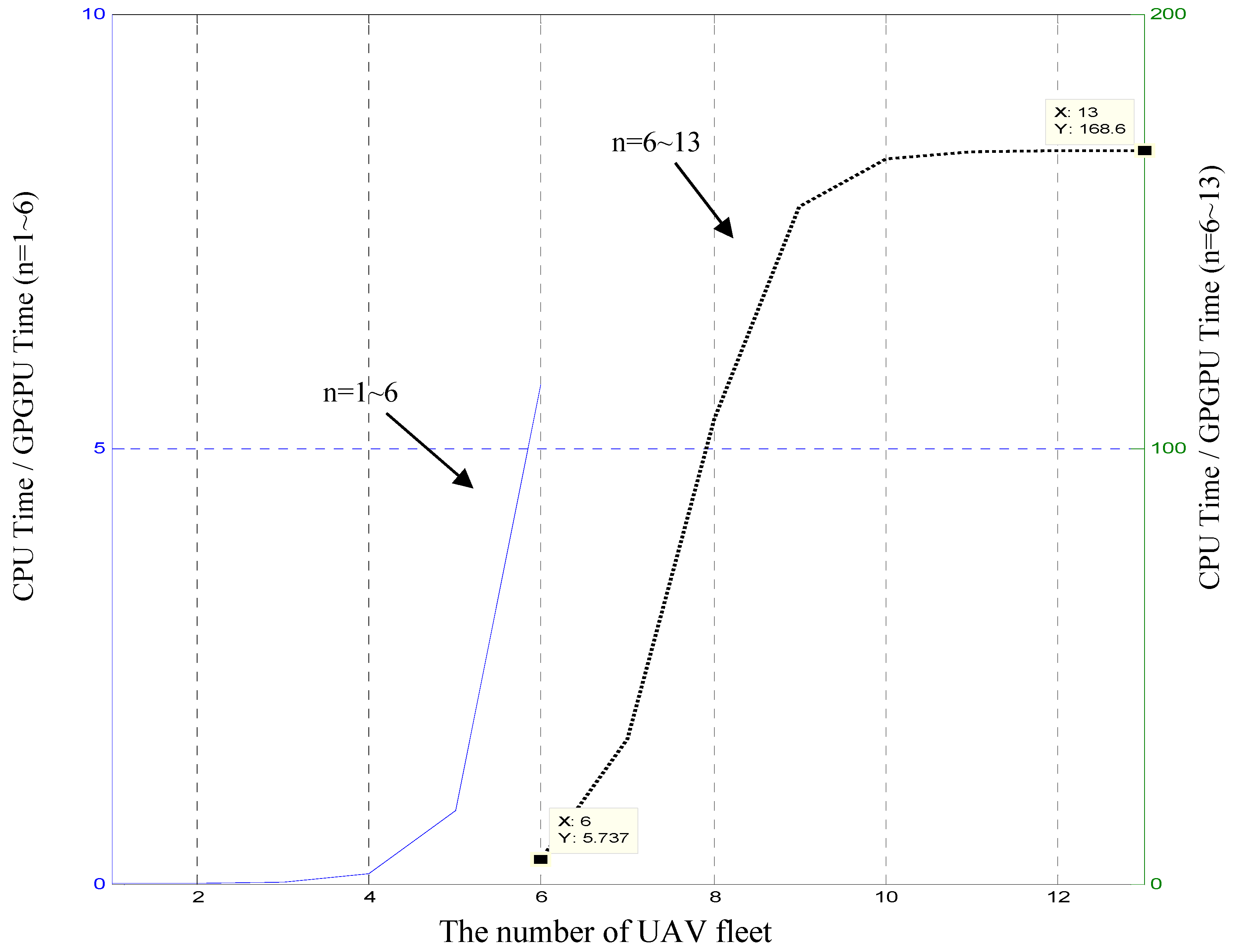
5.4. Ultimate Performance Ratio of CPU/GPGPU
Next, we will speculate on the ultimate Performance ratio. First, use Table 3 and Table 4 to calculate the two models of CPU calculation time and GPGPU calculation time. Assuming that both are linear models, the data transfer time for GPGPU is assumed to be constant, and the data transfer time by the CPU can be ignored. The CPU calculation time model can indicate
GPU calculation time model can represented as
where represents the number of our or enemy fleet in air combat. For the estimation of the coefficient and , this paper uses the regression statistic, the F statistic (hypothesis test for all regression coefficients of zero), the p-value associated with the F statistic, and the estimated value of the error variance. R2 was calculated to be 0.9922, indicating that the model (27) accounted for more than 99% of the variability of the observations from Table 3 and Table 4. The F statistic is about 510 and its p-value is 0.00002, indicating that all regression coefficients and are unlikely to be zero. An error variance of 0.0001 indicates a small random variability between the variable and the regression function (27).
The calculation of is relatively simple. The CPU calculation time in Table 3 is divided by and the CPU calculation time in Table 4 is divided by to obtain observations. The average of the six data is ms, and the error values of 2 × 2 and 4 × 4 are too large (12% and 51%). This data is not credible. Therefore, take the four data in Table 4 and take the average value of ms. Now let (26) and (27) do the performance ratio of , drawing the below Figure 8.
The left coordinate shows the performance ratio of , and the right coordinate shows the performance ratio of . Observed by the solid line, it is true that when is greater than or equal to 6, the GPU computing time will be less than the CPU. The final value of performance ratio falls to 168.5797 times as shown in dashed line. We should emphasize that the results in terms of computational performance could be further improved by using a more powerful GPU in recent years. This is because the GTX285 used in this article is based on the old Tesla architecture with a computing capability of 1.3; while NVIDIA has introduced Kepler, Maxwell, Pascal, and Volta architectures after Tesla and Fermi architecture, these architectures have significantly improved performance. For example, the popular GTX750 microarchitecture is Maxwell with a computing capability of 5.2; the recent TITAN V’s microarchitecture is Volta, and its compute capability reaches 7.
5.5. Performance Comparison of Single Core with Integrated Parallelization
Finally, we tested the CPU decentralization calculations and join CUDA technology. The results are shown in Table 5. It can be found that regardless of the two vs. two or four vs. four fleet simulation, the advantages of decentralized operations are completely eliminated due to the impact of CUDA, which in turn leads to an increase in overall computing time. The main reason may come from:
- (1)
- The number of clusters is too small to really exert the computing power that the GPGPU should have.
- (2)
- In the process of simulation, each time the loop must transfer data from the memory on the motherboard to the memory on the GPGPU, it will waste a lot of time;
- (3)
- In the current hardware of GPGPU, the calculation core of single precision floating point operation is more than the calculation core of double precision floating point operation. For GTX285, the operation core of single precision floating point number is 240, but the operation core of double precision floating point number is only 30, which is eight times worse, so in the MATLAB environment, double precision must be converted to single precision, so it will increase a lot of time to do this conversion;
- (4)
- Parallel computing has its disadvantages to determine the maximum value. In a single core algorithm, we use the zeroth element as a basis to compare with other elements. Therefore, we only need to read other elements, and then write the result to the zeroth element, so only one reading and one writing. However, in the framework of parallelism, the action of comparing two data is double reading and one writing. Therefore, the algorithm of the parallel operation is inherently more computationally intensive than the single-core operation.
6. Conclusions
This paper studies cluster UAV cooperative air combat simulations. Negotiating theory is combined with game theory in order to enhance group superiority. To speed-up computations, this paper used a mixed MATLAB and CUDA C approach. This paper tests the parallel operation of UAV cluster air combat simulation and tests respectively: parallelizes the CPUs of the equations of motion of the two warring parties, the missiles of the warring parties guide using CPU parallelization, and the CPU decentralization calculations joining CUDA technology. The results show that the parallelization of the GPGPU is affected by the number of elements of the strategy matrix and has different performance, when the number of UAVs on the battlefield is too small, the GPGPU’s performance is worse than that of the CPU. However, when there are more than six-to-six combatants, the performance of the GPGPU can be revealed. Therefore, we can regard the six vs. six air combat simulation as a dividing line. When the cluster air combat simulation, the total number of UAVs on both sides is less than 12, one can choose to use CPU parallelism to calculate the equations of motion and strategic decisions for UAVs of the two armies; when there are more than six aircrafts on each side, in addition to parallelizing the equations of motion of the two armies, the choice of strategy in the calculation, we can join the CUDA parallelization acceleration, which can reduce more calculation time.
This is the first way to build a GPU-based multi-UAV maneuver decision-making system for MATLAB to improve its performance by leveraging the huge potential of CUDA. Another noteworthy feature of this work is the use of off-the-shelf components, the Intel Core 2 Quad Q9450 processor (released in 2008) and CUDA-enabled GPUs, GTX285 (240 cores, 648MHz, produced in 2009), as a cost-effective solution to test the architecture of MATLAB mixed C++/CUDA for multi-UAV air combat. Although the equipment is old, many interesting phenomena as described above are still observed and the ultimate performance is forecasted 169 times under the architecture proposed in this paper, which verified the feasibility of the architecture. The results of computational performance in this paper can be further improved by using a more powerful GPU (or multiple GPUs). For example, Intel i5 (eighth generation, manufactured in 2015) and NVIDIA GTX 750 (512 cores, 1020 MHz) is a combination of devices that are now reasonably priced and new in GPU architecture.
Although this article has written CUDA functions and mixed into MATLAB to increase the computational efficiency, but the memory delay problem of MATLAB has not been considered. How to use CUDA different types of memory (such as global, texture, and constant) to get the maximum performance of MATLAB is a feasible direction to avoid performance bottlenecks in the future. Parallel Computing Toolbox on MATLAB makes it easy to solve computational and data-intensive problems with multi-core processors, GPUs, and computer clusters. How the architecture of this article compares performance with Parallel Computing Toolbox should be an interesting question. Apart from that, the CUDA program written in this article has a large number of floating-point matrix multiplications and additions, but has not yet called the CUBLAS library. In the future, CUDA code can be rewritten to call the CUBLAS library to increase performance. On the other hand, MATLAB’s loop execution is slower than other language compilers, if the architecture of this study has to be implemented in real multi-UAV air combat, it is necessary to rewrite the code in other languages (such as C++).
The architecture proposed in this paper can be applied to the existing flight simulator to enhance the intelligent target generation system, assist the pilot in the simulator against the crew, and evaluate the tactics and forecast air combat results, which will help to develop a larger air combat training and evaluation system. However, it can be seen from the research in this paper that although the calculation of maneuvering decision based on matrix game is not difficult, as the number of air combat parties increases, the decision matrix will explode. Even with GPU acceleration, the decision time will be too long. The matrix game method is not suitable for complex real-time air combat environments. Others, such as neural networks or deep learning, may be a better choice.
Funding
This research was funded by Ministry of Science and Technology grant number NSC 99-2221-E-606-008. And the APC was funded by National Defense University.
Acknowledgments
The author would like to thank the research assistants Su,Kuan-chang and Chiang,Feng-Lung for helping to edit, write and test the program in this article, as well as the execution and testing of some experimental results. The author would also like to thank reviewers for their constructive comments and editors for their revision and assistance with this article.
Conflicts of Interest
The authors declare no conflicts of interest.
References
- Austin, F.; Carbone, G.; Hinz, H.; Lewis, M.; Falco, M. Game theory for automated maneuvering during air-to-air combat. J. Guid. Control Dyn. 1990, 13, 1143–1147. [Google Scholar] [CrossRef]
- Burgin, G.; Sidor, L.B. Rule-Based Air Combat Simulation; Technical Report, TITAN-TLJ-H-1501; Titan Systems Inc.: La Jolla, CA, USA, 1988. [Google Scholar]
- Virtanen, K.; Karelahti, J.; Raivio, T. Modeling air combat by a moving horizon influence diagram game. J. Guid. Control Dyn. 2006, 29, 1080–1091. [Google Scholar] [CrossRef]
- Virtanen, K.; Raivio, T.; Hamalainen, R.P. Modeling pilot’s sequential maneuvering decisions by a multistage influence diagram. J. Guid. Control Dyn. 2004, 27, 665–677. [Google Scholar] [CrossRef]
- Xie, R.Z.; Li, J.Y.; Luo, D.L. Research on maneuvering decisions for Multi-UAVs air combat. In Proceedings of the 2014 IEEE International Conference Control & Automation, Taichung, Taiwan, 18–20 June 2014; pp. 767–772. [Google Scholar]
- Pan, Q.; Zhou, D.; Huang, J.; Lv, X.; Yang, Z.; Zhang, K.; Li, X. Maneuver decision for cooperative close-range air combat based on state predicted influence diagram. In Proceedings of the 2017 IEEE International Conference on Information and Automation, Macau, China, 18 July 2017; pp. 726–731. [Google Scholar]
- Liu, B. Air combat decision making for coordinated multiple target attack using combinatorial auction. Acta Aeronaut. Astronaut. Sin. 2010, 31, 1433–1444. [Google Scholar]
- Song, X.; Jiang, J.; Xu, H. Application of improved simulated annealing genetic algorithm in cooperative air combat. J. Harbin Eng. Univ. 2017, 38, 1762–1768. [Google Scholar]
- Ding, Y.; Yang, L.; Hou, J.; Jin, G.; Zhen, Z. Multi-target collaborative combat decision-making by improved particle swarm optimizer. Trans. Nanjing Univ. Aeronaut. Astronaut. 2018, 35, 181–187. [Google Scholar]
- Sun, T.Y.; Tsai, S.J.; Huo, C.L. Intelligent maneuvering decision system for computer generated forces using predictive fuzzy inference system. J. Comput. 2008, 3, 58–66. [Google Scholar] [CrossRef]
- Roessingh, J.J.; Merk, R.J.; Huibers, P.; Meiland, R.; Rijken, R. Smart bandits in air-to-air combat training: Combining different behavioural models in a common architecture. In Proceedings of the 21st Annual Conference on Behavior Representation in Modeling and Simulation, Amelia Island, FI, USA, 12–15 March 2012. [Google Scholar]
- McGrew, J.S.; How, J.P.; Williams, B.; Roy, N. Air-combat strategy using approximate dynamic programming. J. Guid. Control Dyn. 2012, 33, 1641–1654. [Google Scholar] [CrossRef] [Green Version]
- Teng, T.H.; Tan, A.H.; Tan, Y.S.; Yeo, A. Self-organizing neural networks for learning air combat maneuvers. In Proceedings of the 2012 International Joint Conference on Neural Networks, Brisbane, Australia, 10–15 June 2012; pp. 1–8. [Google Scholar]
- Liu, P.; Ma, Y. A Deep reinforcement learning based intelligent decision method for UCAV air combat. In Proceedings of the 17th Asia Simulation Conference, Melaka, Malaysia, 27–29 August 2017; pp. 274–286. [Google Scholar]
- Mnih, V.; Kavukcuoglu, K.; Silver, D.; Rusu, A.A.; Veness, J. Human-level control through deep reinforcement learning. Nature 2015, 518, 529–533. [Google Scholar] [CrossRef] [PubMed]
- Silver, D.; Huang, A.; Maddison, C.J.; Guez, A.; Sifre, L.; Van Den Driessche, G.; Schrittwieser, J.; Antonoglou, I.; Panneershelvam, V.; Lanctot, M.; et al. Mastering the game of Go with deep neural networks and tree search. Nature 2016, 529, 484–489. [Google Scholar] [CrossRef] [PubMed]
- Luo, P.C.; Xie, J.J.; Che, W.F. Q-learning based air combat target assignment algorithm. In Proceedings of the 2016 IEEE International Conference on Systems, Man, and Cybernetics, Budapest, Hungary, 9–12 October 2016; pp. 779–783. [Google Scholar]
- Zuo, J.; Yang, R.; Zhang, Y.; Li, Z.; Wu, M. Intelligent decision-making in air combat maneuvering based on heuristic reinforcement learning. Acta Aeronaut. Astronaut. Sin. 2017, 38, 217–230. [Google Scholar]
- Xu, G.; Zhou, B.; Zhang, H. Multi-player nonzero-sum Nash differential game: Variation and pseudo-spectral method. Optim. Control Appl. Methods 2017, 38, 506–519. [Google Scholar] [CrossRef]
- Sheng, W.; Li, J.; Tong, M.G. Research of differential game theory for multiple consulting air combat. Syst. Eng. Electron. 1998, 20, 7–11. [Google Scholar]
- Wei, S.; Mingan, T.; Honglun, W.; Jianxun, L. Decision and information fusion in multiple air combat. J. Beijing Univ. Aeronaut. Astronaut. 1999, 25, 665–667. [Google Scholar]
- Li, Q.; Yang, R.; Li, H.; Zhang, H.; Feng, C. Research on the non-cooperative game strategy of suppressing IADS for multiple fighters cooperation. J. Xidian Univ. 2017, 44, 129–137. [Google Scholar]
- Selvakumar, J.; Bakolas, E. Evasion with Terminal Constraints from a Group of Pursuers using a Matrix Game Formulation. In Proceedings of the 2017 American Control Conference, Seattle, WA, USA, 24–26 May 2017; pp. 1604–1609. [Google Scholar]
- Xu, H.; Xing, Q.; Wang, W. WTA for air and missile defense based on fuzzy multi-objective programming. Syst. Eng. Electron. 2018, 40, 563–570. [Google Scholar]
- Zhang, Y.; Wu, W.; Wang, J. Interval valued intuitionistic fuzzy Petri net and its application in air combat decision making. Syst. Eng. Electron. 2017, 39, 1051–1057. [Google Scholar]
- Vladimir, T.; Kim, D.H.; Ha, Y.G.; Jeon, D.W. Fast multi-line detection and tracking with CUDA for vision-based UAV autopilot. In Proceedings of the 8th International Conference on Innovative Mobile and Internet Services in Ubiquitous Computing, Birmingham, UK, 2–4 July 2014; pp. 96–101. [Google Scholar]
- Hossain, R.; Magierowski, S.; Messier, G.G. GPU enhanced path finding for an unmanned aerial vehicle. In Proceedings of the IEEE 28th International Parallel and Distributed Processing Symposium Workshops, Phoenix, AZ, USA, 19–23 May 2014; pp. 1285–1293. [Google Scholar]
- Cekmez, U.; Ozsiginan, M.; Sahingoz, O.K. Multi-UAV path planning with parallel genetic algorithms on CUDA architecture. In Proceedings of the Genetic and Evolutionary Computation Conference, Denver, CO, USA, 20–24 July 2016; pp. 1079–1086. [Google Scholar]
- Bonelli, F.; Tuttafesta, M.; Colonna, G.; Cutrone, L.; Pascazio, G. An MPI-CUDA approach for hypersonic flows with detailed state-to-state air kinetics using a GPU cluster. Comput. Phys. Commun. 2017, 219, 178–195. [Google Scholar] [CrossRef]
- Rudianto, I. Spectral-element simulation of two-dimensional elastic wave propagation in fully heterogeneous media on a GPU cluster. In Proceedings of the International Conference on Theoretical and Applied Physics, Vienna, Austria, 2–3 July 2018. [Google Scholar]
- Vigmond, E.J. Near-real-time simulations of biolelectric activity in small mammalian hearts using graphical processing units. In Proceedings of the Annual International Conference of the IEEE Engineering in Medicine and Biology Society, Minneapolis, MN, USA, 3–6 September 2009. [Google Scholar]
- Yang, Z.; Zhu, Y.; Pu, Y. Parallel image processing based on CUDA. In Proceedings of the International Conference on Computer Science and Software Engineering, Hubei, China, 12–14 December 2008. [Google Scholar]
- Grant, M.; Boyd, S. CVX: Matlab Software for Disciplined Convex Programming, Version 2.1. 2017. Available online: Cvxr.com/cvx (accessed on 22 August 2018).
- Sun, Y.Q.; Zhou, X.C.; Meng, S. Research on maneuvering decision for multi-fighter cooperative air combat. In Proceedings of the International Conference on Intelligent Human-Machine Systems and Cybernetics, Hangzhou, China, 26–27 August 2009; pp. 197–200. [Google Scholar]
- Kung, C.C.; Chiang, F.L. A study of missile maximum capture area and fighter minimum evasive range for negotiation team air combat. In Proceedings of the 15th International Conference on Control, Automation and Systems, Busan, Korea, 13–16 October 2015; pp. 207–212. [Google Scholar]
- Weiss, M.; Shima, T. Minimum effort rursuit/evasion guidance with specified miss distance. J. Guid. Control Dyn. 2016, 39, 1069–1079. [Google Scholar] [CrossRef]
- Dollinger, J.F.; Loechner, V. Adaptive runtime selection for GPU. In Proceedings of the 42nd International Conference on Parallel Processing, Lyon, France, 1–4 October 2013; pp. 70–79. [Google Scholar]
- Fatica, M.; Jeong, W.K. Accelerating Matlab with CUDA. In Proceedings of the Eleventh Annual High Performance Embedded Computing Workshop Lexington Massachusetts, Lexington, MA, USA, 18–20 September 2007. [Google Scholar]
- Simek, V.; Asn, R.R. GPU acceleration of 2D-DWT image compression in Matlab with CUDA. In Proceedings of the 2nd UKSim European Symposium on Computer Modelling and Simulation, Liverpool, UK, 8–10 September 2008; pp. 274–277. [Google Scholar]
- Horrigue, L.; Ghodhbane, R.; Saidani, T.; Atri, M. GPU acceleration of image processing algorithm based on Matlab CUDA. Int. J. Comput. Sci. Netw. Secur. 2018, 18, 91–99. [Google Scholar]
- Austin, F.; George, D. Automated adversary for piloted simulation of helicopter air combat in terrain flight. J. Am. Helicopter Soc. 1992, 37, 25–31. [Google Scholar] [CrossRef]
- Elsayed, A. Modeling of a small unmanned aerial vehicle. Int. J. Aerosp. Mech. Eng. 2015, 9, 503–511. [Google Scholar]
- Kung, C.C.; Chiang, F.L.; Wu, C.Y. Implement three-dimensional pursuit guidance law with feedback linearization control method. Int. J. Mech. Aerosp. Ind. Mechatron. Manuf. Eng. 2011, 5, 1201–1217. [Google Scholar]
- Ostlund, P.; Stavaker, K.; Fritzson, P. Parallel simulation of equation-based models on CUDA-enabled GPUs. In Proceedings of the Parallel/High-Performance Object-Oriented Scientific Computing, Reno, NV, USA, 17–21 October 2010. [Google Scholar]
- Al-Omari, A.; Arnold, J.; Taha, T.; Schüttler, H.-B. Solving large nonlinear systems of ODE with hierarchical structure using multi-GPGPUs and an adaptive Runge Kutta. IEEE Access 2013, 1, 770–777. [Google Scholar] [CrossRef]
- Seen, W.M.; Gobithaasan, R.U.; Miura, K.T. GPU acceleration of Runge Kutta-Fehlberg and its comparison with Dormand-Prince method. AIP Conf. Proc. 2014, 1605, 16–21. [Google Scholar]
- Oberhuber, T.; Suzuki, A.; Žabka, V. The CUDA implementation of the method of lines for the curvature dependent flows. Kybernetika 2011, 47, 251–272. [Google Scholar]
Figure 1.
Flowchart of collaborative mission for UAV cluster.

Figure 2.
(a) Fighter flight strategies; (b) representation of the fighter in the local reference frame XYZ.
Figure 2.
(a) Fighter flight strategies; (b) representation of the fighter in the local reference frame XYZ.

Figure 3.
Flowchart of team negotiation decision.

Figure 4.
Flowchart for each fighter deciding attack/escape and role in a team.

Figure 5.
Mixed parallel computing framework of graphics processing unit.

Figure 6.
2 × 2 drone aircraft air combat simulation.

Figure 7.
2 × 2 unequal air combat simulation.

Figure 8.
Plot of performance ratio (CPU time/GPGPU time).


Table 1.
Strategy and command value.
| Strategy | Strategy 1 | Strategy 2 | Strategy 3 | Strategy 4 | Strategy 5 | Strategy 6 | Strategy 7 | |
|---|---|---|---|---|---|---|---|---|
| Command Values | Max Load Factor Left Turn | Max Long Acceleration | Steady Flight | Max Long Deceleration | Max Load Factor Right Turn | Max Load Factor Pull Up | Max Load Factor Push Over | |
| (g) | 0 | 1.5 | 0 | −1.5 | 0 | 0 | 0 | |
| (g) | 3 | 0 | 0 | 0 | 3 | 3 | −3 | |
| (rad) | 0 | 0 | 0 | 0 | 0 | |||
Table 2.
Test hardware specifications.
| Component Type | Component |
|---|---|
| CPU | Intel Core 2 Quad [email protected] |
| Operating system | Windows 7 |
| GPU | GTX285 |
| GPU cuda cores | 240 |
| CPU memory | 12.0 GB |
| GPU memory | 1 GB |
| CPU compiler | VC++ 2010 |
| GPU compiler | NVCC 4.0 |
Table 3.
Comparison of calculation time after selecting CUDA.
| Number of Clusters | CPU Calculation Time (ms) Q9450 | GPGPU Calculation Time (ms) GTX285 |
|---|---|---|
| 2 × 2 | 0.016168 | 5.41302 |
| 4 × 4 | 20.6626 | 282.696 |
Table 4.
Performance ratio of CPU/GPGPU.
| Row Number | CPU Calculation Time (ms) Q9450 | GPGPU Calculation Time (ms) GTX285 | Performance Ratio (CPU Time/GPGPU Time) |
|---|---|---|---|
| 0.0967 | 0.1088 | 0.0888 | |
| 0.6592 | 0.1087 | 6.064 | |
| 4.6257 | 0.1515 | 30.53 | |
| 33.3234 | 0.3058 | 108.97 |
Table 5.
Comparison of integrated parallelization simulation time.
| Cluster Number | Single Core Calculation (s) | Decentralized Calculation and Join CUDA (s) |
|---|---|---|
| 2 vs. 2 | 25.058792 | 30.456212 |
| 4 vs. 4 | 198.9946 | 398.4786 |
© 2018 by the author. Licensee MDPI, Basel, Switzerland. This article is an open access article distributed under the terms and conditions of the Creative Commons Attribution (CC BY) license (http://creativecommons.org/licenses/by/4.0/).
Share and Cite
MDPI and ACS Style
Kung, C.-C. Study on Consulting Air Combat Simulation of Cluster UAV Based on Mixed Parallel Computing Framework of Graphics Processing Unit. Electronics 2018, 7, 160. https://doi.org/10.3390/electronics7090160
AMA Style
Kung C-C. Study on Consulting Air Combat Simulation of Cluster UAV Based on Mixed Parallel Computing Framework of Graphics Processing Unit. Electronics. 2018; 7(9):160. https://doi.org/10.3390/electronics7090160
Chicago/Turabian StyleKung, Chien-Chun. 2018. "Study on Consulting Air Combat Simulation of Cluster UAV Based on Mixed Parallel Computing Framework of Graphics Processing Unit" Electronics 7, no. 9: 160. https://doi.org/10.3390/electronics7090160
Note that from the first issue of 2016, this journal uses article numbers instead of page numbers. See further details here.