FPGA Implementation of a Functional Neuro-Fuzzy Network for Nonlinear System Control

Abstract

This study used Xilinx Field Programmable Gate Arrays (FPGAs) to implement a functional neuro-fuzzy network (FNFN) for solving nonlinear control problems. A functional link neural network (FLNN) was used as the consequent part of the proposed FNFN model. This study adopted the linear independent functions and the orthogonal polynomials in a functional expansion of the FLNN. Thus, the design of the FNFN model could improve the control accuracy. The learning algorithm of the FNFN model was divided into structure learning and parameter learning. The entropy measurement was adopted in the structure learning to determine the generated new fuzzy rule, whereas the gradient descent method in the parameter learning was used to adjust the parameters of the membership functions and the weights of the FLNN. In order to obtain high speed operation and real-time application, a very high speed integrated circuit hardware description language (VHDL) was used to design the FNFN controller and was implemented on FPGA. Finally, the experimental results demonstrated that the proposed hardware implementation of the FNFN model confirmed the viability in the temperature control of a water bath and the backing control of a car.

1. Introduction

Neural fuzzy networks (NFNs) have been widely applied in various fields [1,2,3]. Traditional NFNs combine neural networks to learn from processes with fuzzy reasoning to handle uncertain information. These can only be applied to parameter learning based on the ordered derivative algorithm where the structure of the NFNs has been determined and fixed in advance [4,5,6]. In [7,8], a neuro-fuzzy system could learn system behavior from the training data and automatically generate fuzzy rules and fuzzy sets to a prespecified accuracy level. The major disadvantage of the existing neural fuzzy networks is that their application is limited to static problems as a result of their internal feedforward network structure. For TSK-type neural fuzzy networks (TNFNs), the consequent part of each fuzzy rule is a linear combination of the input variable. However, the traditional TNFN cannot use the mapping capabilities of the linear function combination in consequent parts of the fuzzy rules. Hence, the FNFN model, which combines a neuro-fuzzy network with a FLNN [9], was proposed to improve the accuracy of functional approximation. Corresponding to a FLNN, each fuzzy rule comprises a functional expansion of inputs. The linearly independent functions and orthogonal polynomials are used in FLNN. The learning algorithm was divided into structure learning and parameter learning and used for constructing the FNFN automatically. Initially, no rules existed in the FNFN model. In the structure learning algorithm, the entropy measure was used to determine a whether a new node needed to be added. In the parameter learning, the backpropagation leaning method was used to adjust the parameters of the FNFN model.

Real-time control is very important in industrial process control system applications. For rapid computing hardware engineering, real-time control becomes more feasible [10]. Recently, there has been a focus on the hardware implementation [11] of artificial neural networks (ANNs). Furthermore, the realization that a hybrid of neural networks and fuzzy systems presents an even more powerful form of computational intelligence [12] provides additional motivation to complete hardware implementation. The main reason for hardware implementation is that it has high speed processing and real-time operating capability. In many applications, hardware implementation requires larger arrays and has resorted to digital simulation, which are usually built using digital integrated circuits. Development of digital integrated circuits such as FPGA [13] makes the hardware implementation process programmable and flexible. Recently, the hardware implementation of neural networks has been successfully implemented. Li et al. [10] discussed various aspects of the hardware implementation of an artificial neural network (ANN), e.g., generic architecture, back propagation, precision, etc. One of the best arguments for hardware is the exploitation of parallelism in the neural network, which can be very fast, especially for well-defined signal processing usage. They implemented basic ANN in field programmable gate arrays (FPGA). Compared to software, FPGA implementation can utilize parallelism to speed up processing time. Page and Mohsenin [11] reduced complexity, efficiently deployed deep networks in an embedded FPGA-based setting with strict power and area budgets and reduced the inherent complexity of a network by applying both fixed-point quantization and low-rank weight approximation. Bettoni et al. [13] presented an FPGA implementation of Convolutional Neural Networks (CNN) designed for addressing portability and power efficiency for video processing applications such as video surveillance and homeland security. However, their implementation using hardware resulted in a lack of learning ability. According to the aforementioned disadvantages, this study presented the hardware implementation of FNFN using FPGAs to solve nonlinear control problems.

This study is organized as follows. The related work is introduced in Section 2. The FNFN structure is presented in Section 3. The structure and parameter learning algorithms are illustrated in Section 4. Next, Section 5 describes the FPGA hardware implementation of the FNFN controller. The experimental results of two nonlinear control applications are described in Section 6. Finally, the conclusions are given in the last section.

2. Related Work

Recently, many algorithms have been implemented on FPGA for real-time applications [14,15,16,17]. Emanuel et al. [18] proposed a fuzzy logic edge detector based on the morphological gradient for pattern recognition and realized on FPGA. The hardware architecture processing the image resolution was set to 480 × 640 pixels at 24 fps, and the hardware architecture enables handling the real-time processing for an image resolution set to 480 × 640 pixels at 24 fps. Ammar et al. [19] designed a sun tracking system by a using neuro-fuzzy controller implemented on FPGA. The experimental results revealed that the neuro-fuzzy controller was more robust than the fuzzy logic controller. M. et al. [20] presented the design and implementation of a low-cost solar-powered wheelchair for physically challenged people. They constructed an artificial neural network-based classifier to classify the patterns and features extracted from the raw sEMG signals; and the proposed wheelchair revealed that it was financially feasible and cost-effective. Yesid et al. [21] presented a neuro fuzzy controller for a robot that rode a bicycle using the Acrobot model for slow speeds, which was also implemented on an FPGA-based embedded system.

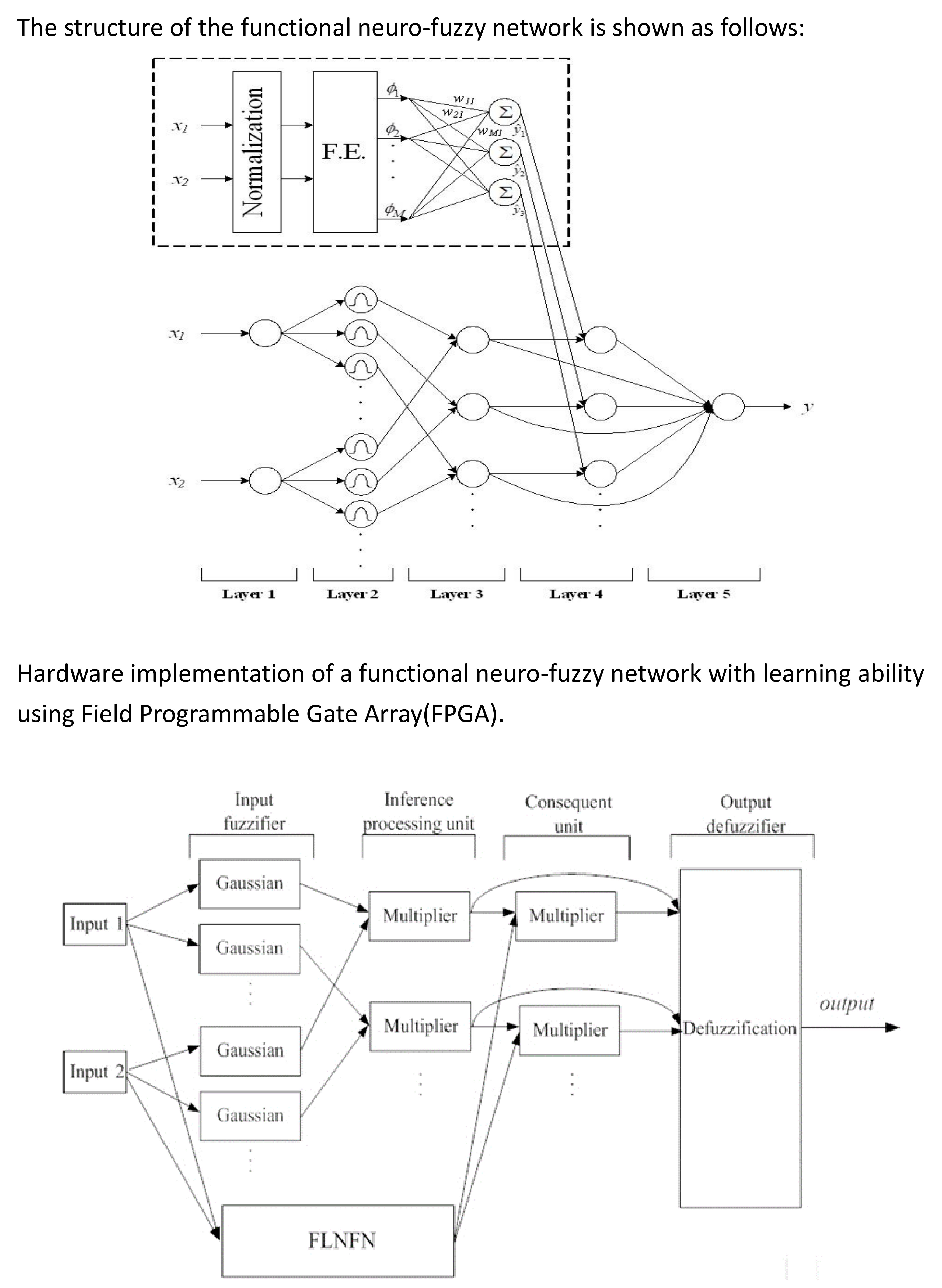
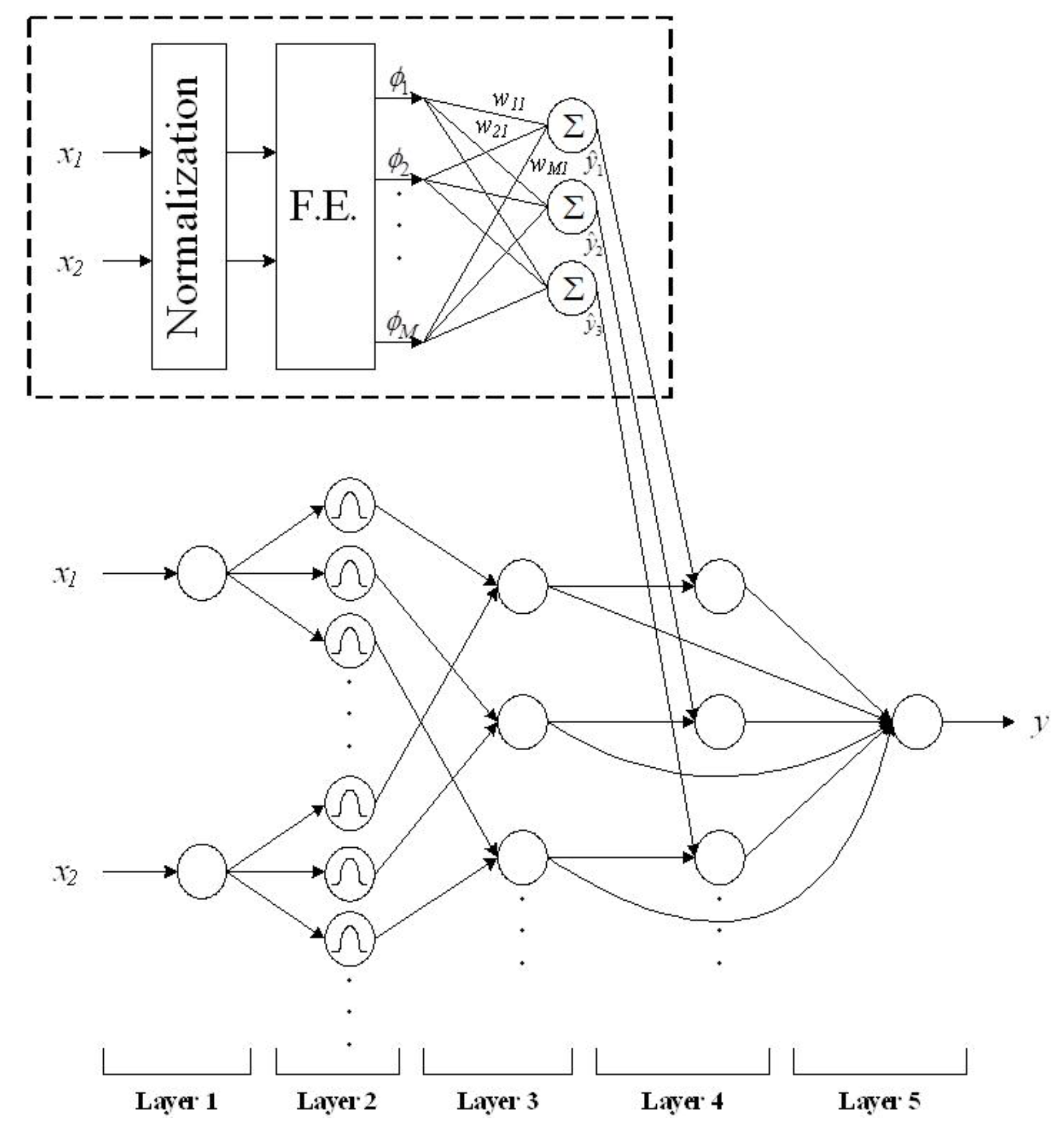
3. Architecture of Functional Neuro-Fuzzy Networks (FNFN)

In the proposed FNFN model, the function link neural network (FLNN) was used as the concluding part of a fuzzy rule. The FLNN adopts a nonlinear combination of input variables. The architecture of a FNFN model is shown in Figure 1.

The jth fuzzy if-then rule in FNFN model is described as follows.

$$\mathrm{IF}{x}_{1}is{B}_{ij}and{x}_{2}is{B}_{2j}\cdots and{x}_{i}is{B}_{ij}\cdots and{x}_{N}is{B}_{Nj,}THEN{y}_j={\displaystyle \sum }_{k=1}^M{w}_{kj}{\varnothing }_k$$

(1)

where x_i represents the input; y_j is the output of the jth fuzzy rule; B_ij represents the membership function; w_kj denotes the link weight; N denotes the number of input variables; M presents the basis function number; and $\varnothing$_k represents the trigonometric polynomial function combination of input variables.

Next, we describe the FNFN architecture layer by layer. In layer 1, no operation exists and the input signals transmit to the second layer directly:

$$u_i^{(1)}=x_i$$

(2)

where A_ij presents a membership function. In layer 2, we adopted a Gaussian membership function for FNFN, which had the following advantages: (1) a small number of parameters are needed to define; (2) better robustness; and (3) the performance is superior than polygonal membership functions. The degree of the membership function is calculated

$$u_{ij}^{(2)}=\exp \left(-\frac{{\left[u_i^{(1)}-m_{ij}\right]}^2}{{\sigma }_{ij}^2}\right)$$

(3)

where m_ij and σ_ij represent the expected value and variance, respectively.

In layer 3, the product operator is used to achieve the conditional part in the fuzzy rules. Outputs are described as follows:

$$u_j^{(3)}={\displaystyle \prod _i{u}_{ij}^{(2)}}$$

(4)

where ${\displaystyle \prod _i{u}_{ij}^{(2)}}$ denotes the inference of its corresponding rule.

In Figure 1, the outputs of layer 3 were used as the inputs of layer 4, and the other inputs in layer 4 were from the outputs of a FLNN. The node in layer 4 is illustrated as follows:

$$u_j^{(4)}=u_j^{(3)}\cdot {\displaystyle \sum _{k=1}^M{w}_{kj}{\varphi }_k}$$

(5)

The functional expansion (F.E.) adopts a trigonometric polynomial basis function and is described by $\varnothing$_k = [x₁,sin(πx₁), cos(πx₁), x₂,sin(πx₂),cos(πx₂), x₁ x₂] for two-dimensional input variables.

In layer 5, the output of the FNFN is a defuzzification operation

$$y=u^{(5)}=\frac{{\displaystyle \sum _{j=1}^R{u}_j^{(4)}}}{{\displaystyle \sum _{j=1}^R{u}_j^{(3)}}}=\frac{{\displaystyle \sum _{j=1}^R{u}_j^{(3)}\left({\displaystyle \sum _{k=1}^M{w}_{kj}{\varphi }_k}\right)}}{{\displaystyle \sum _{j=1}^R{u}_j^{(3)}}}=\frac{{\displaystyle \sum _{j=1}^R{u}_j^{(3)}{\widehat{y}}_j}}{{\displaystyle \sum _{j=1}^R{u}_j^{(3)}}}$$

(6)

where R and y represent the fuzzy rule number and the output of the FNFN model, respectively.

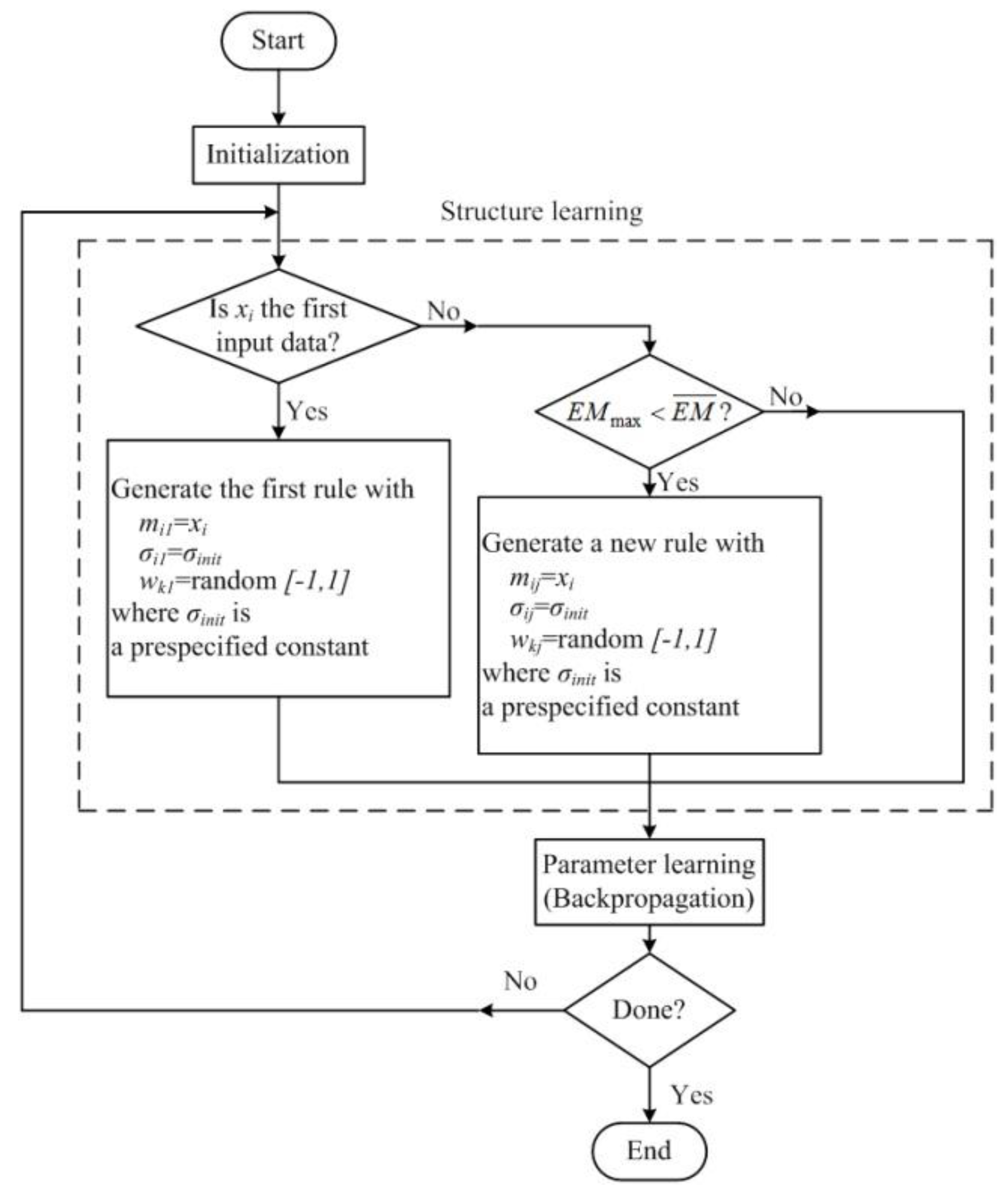
4. Proposed Learning Algorithm

In this study, the proposed learning algorithm was comprised of structure learning and parameter learning. The flowchart of the proposed learning algorithm is shown in Figure 2. By satisfying the fuzzy partitioning of the input variables, the entropy measurement was used to decide the fuzzy rule number in the structure learning. In parameter learning, the gradient descent method was used to minimize the error function by adjusting the parameters in the FNFN.

4.1. Structure Learning

In structure learning, the generated fuzzy rules are decided by the training data. The entropy measurement is adopted to measure the similarity between each membership function and each input data. If the input data is close to the mean of a membership function, it has a lower entropy value. This means that the entropy values are computed to decide whether or not a new fuzzy rule is added. The entropy measurement is determined by the firing degree.

$$S_j=-{\displaystyle \sum }_{i=1}^N{F}_{ij}lo{g}_2{F}_{ij}$$

(7)

where $F_{ij}=\exp (u_{ij}^{{\left(2\right)}^{-1}})$ and S_j is between zero and one. The maximum entropy measurement is described as follows:

$$S_{max}=\underset{1\le j\le R}{\max }{S}_j$$

(8)

where R represents the current rule number. If $S_{max}\le \overline{S}$, then a new fuzzy rule is added. The value of $\overline{S}$ is a pre-defined threshold value and is between zero and one. Its value will decay during the learning process.

During structure learning, the $\overline{S}$ value is an important parameter to determine whether a new fuzzy rule is generated. In general, the $\overline{S}$ value is pre-defined as 0.3 × N, where N denotes the number of inputs.

If a new fuzzy rule has been added, the initial expected value, variance, and weights of a new generated fuzzy rule are determined in the next step. As the learning target is to minimize the error function, the expected value, variance, and weights are adjusted as follows:

$$m_{ij}=x_i$$

(9)

$${\sigma }_{ij}={\sigma }_{init}$$

(10)

$$w_{jk}\in \left[0,1\right]$$

(11)

where x_i represents the current input data and σ_init denotes a pre-defined value.

4.2. Parameter Learning

According to the current input data, the structure of the FNFN model has been adjusted. Next, the model goes into parameter learning to adjust the parameters of the FNFN model based on the same input data. The goal of parameter learning is to minimize the error function. The gradient descent method is used for this backpropagation (BP) learning. For a single output condition, the target of BP is to minimize the error function as follows:

$$\mathrm{E}\left(k\right)=\raisebox{1ex}{$1$}\!\left/ \!\raisebox{-1ex}{$2$}\right.{(y\left(k\right)-y^d\left(k\right))}^2=\raisebox{1ex}{$1$}\!\left/ \!\raisebox{-1ex}{$2$}\right.e^2\left(k\right)$$

(12)

where y^d(t) and y(t) are the goal output and the actual output for time t, respectively.

The parameters of the FNFN model can be adjusted by using the BP learning algorithm and are defined as follows:

$$w\left(k+1\right)=w\left(k\right)-\eta \frac{\partial E\left(k\right)}{\partial w\left(k\right)}$$

(13)

where η denotes the learning rate. W = [m, σ, w]^T denotes the adjustable parameters of the FNFN. The BP of the adjustable parameters W is derived as follows:

$$\frac{\partial E\left(k\right)}{\partial w}=e\left(k\right)\frac{\partial y\left(k\right)}{\partial w}$$

(14)

The adjustable parameters in the FNFN model are adjusted by the chain rule in each layer. The updating rule for w_j is derived as follows:

$$w_{kj}\left(k+1\right)=w_{kj}\left(k\right)-{\eta }_{w}e\left(\frac{u_j^{\left(3\right)}{\varnothing }_k}{{{\displaystyle \sum }}_{j=1}^R{u}_j^{\left(3\right)}}\right)$$

(15)

Similarly, the updating rule for m_ij and σ_ij are derived as follows:

$$m_{ij}\left(k+1\right)=m_{ij}\left(k\right)-{\eta }_{m}e(\frac{u_j^{\left(4\right)}}{{{\displaystyle \sum }}_{j=1}^R{u}_j^{\left(3\right)}})(\frac{2\left(u_i^{\left(1\right)}-m_{ij}\right)}{{\sigma }_{ij}^2})$$

(16)

$${\sigma }_{ij}\left(k+1\right)={\sigma }_{ij}\left(k\right)-{\eta }_{\sigma }e(\frac{u_j^{\left(4\right)}}{{{\displaystyle \sum }}_{j=1}^R{u}_j^{\left(3\right)}})(\frac{2(u_i^{\left(1\right)}-m_{ij})}{{\sigma }_{ij}^3})$$

(17)

where η_w, η_m, and η_σ are the learning rates of the weight, the expected value, and the variance, respectively.

5. FPGA Implementation of the FNFN Controller

This section introduces the overall hardware detail design and implementation of the FNFN controller. This section illustrates the represented fixed-point data format. The various function units are implemented by Taylor expansion and look-up table (LUT) methods including Gaussian function, sine function, and cosine function. In this section, the hardware implementation overall components of the FNFN controller are also introduced and are shown in Figure 3. Four main parts can be described as follows: (A) Input fuzzifier; (B) Inference processing unit; (C) Consequent unit; and (D) Output defuzzifier. Finally, the FPGA development platform is introduced.

5.1. The Represented Data Format

In order to keep the represented data format consistent in the FNFNs, a fixed-point number was adopted. An encoding technology adopted digital values to illustrate the represented data [8]. The represented fixed-point data format can be denoted as follows:

$$\left[b\right]i·f$$

(18)

where b represents a sign bit. If b is equal to 0, the value is a positive number, whereas if b is equal to 1, the value is a negative number. i and f denote the numbers of integer bits and fractional bits, respectively [9,10]. Twenty bits were adopted as the number of a word length in this study and had more accuracy than 16 bits. The fixed-point data format included 1 sign bit, 6 integer bits, and 13 fractional bits.

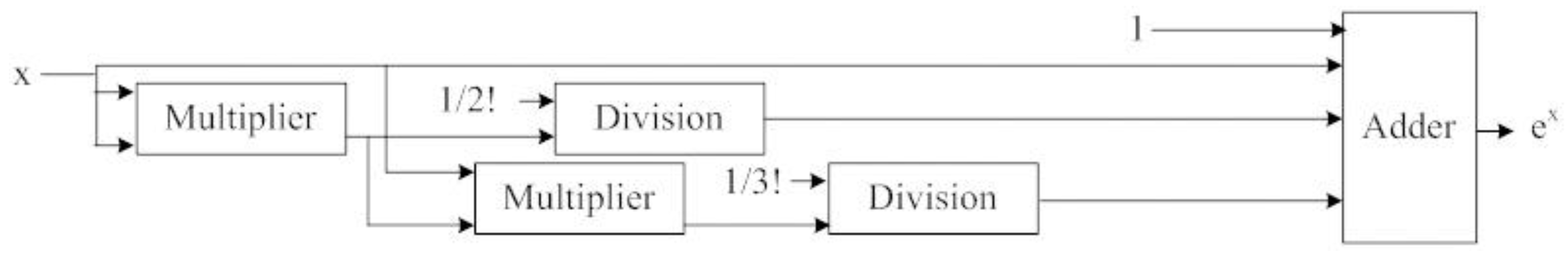
5.2. Design and Implementation of Function Unit

First of all, in the process of hardware implementation of the FNFN, the problem in the implemented exponential of the Gaussian function of the TSK-type fuzzy model (Figure 3), sine function of FLNN, and cosine function of FLNN will occur (Figure 4). The functions are complex and not easily accomplished directly with FPGA implementation. Therefore, the LUT and Taylor expansion were used to approach the Gaussian function, sine function, and cosine function.

The Taylor expansion is shown in Equations (19)–(21), and its advantage is that it only utilizes simple operations which can accurately answer. The disadvantage of LUT is that it must obtain the correspondence of the input and output value of each datum in advance when setting up the table, so it takes a much longer time.

$$e^x=1+\frac{x}{1!}+\frac{x^2}{2!}+\frac{x^3}{3!}+\dots +\frac{x^n}{n!}={\displaystyle \sum _{n=0}^{\infty }\frac{x^n}{n!}}$$

(19)

$$\sin x=x-\frac{x^3}{3!}+\frac{x^5}{5!}-\frac{x^7}{7!}+\dots ={\displaystyle \sum _{n=0}^{\infty }{\left(-1\right)}^n\frac{x^{2n+1}}{\left(2n+1\right)!}}$$

(20)

$$\cos x=1-\frac{x^2}{2!}+\frac{x^4}{4!}-\frac{x^6}{6!}+\dots ={\displaystyle \sum _{n=0}^{\infty }{\left(-1\right)}^n\frac{x^{2n}}{\left(2n\right)!}}$$

(21)

where x is the input variable and n is the number of order. If n is a large order, a more accurate approach will be obtained. In this case, it needs more memory spaces and logic gates.

Table 1. The error value of exponential function and Taylor approximation.

	Method	Exponential Function (x = 0.8)	Taylor Approximation	Error Value
Order
3		2.225541	2.205330	0.020208
4			2.222400	0.003141
5			2.225131	0.000410

shows the error value of the exponential function and Taylor approximation as the higher order requires more complicated operations. In this study, we chose order n = 3 to achieve the e^x, sin x, and cos x hardware.

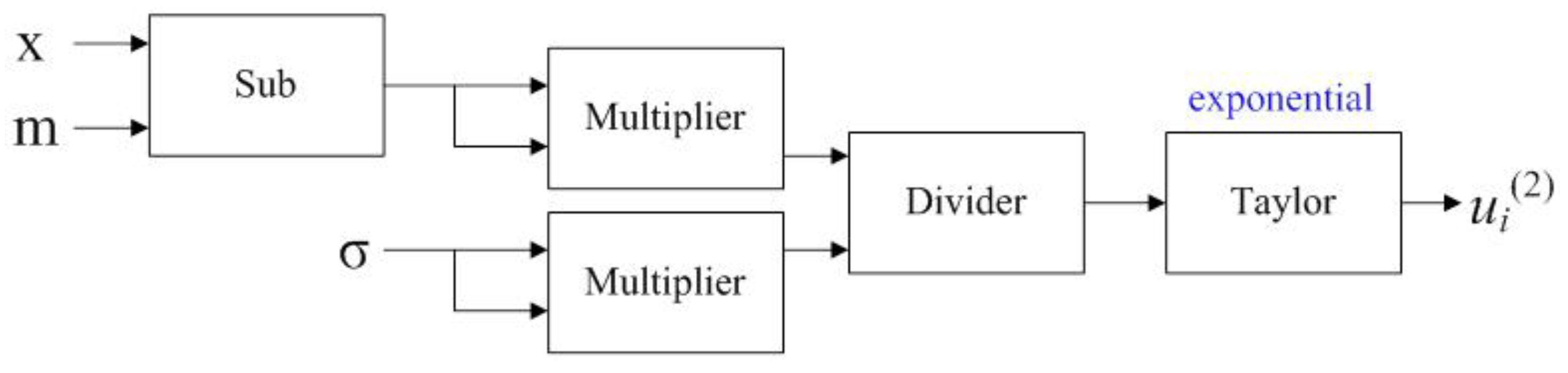
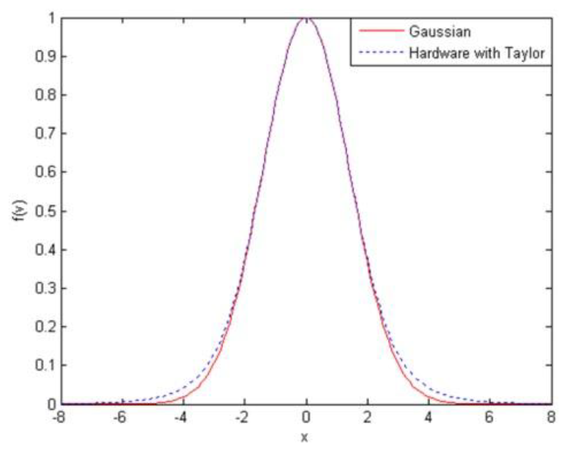
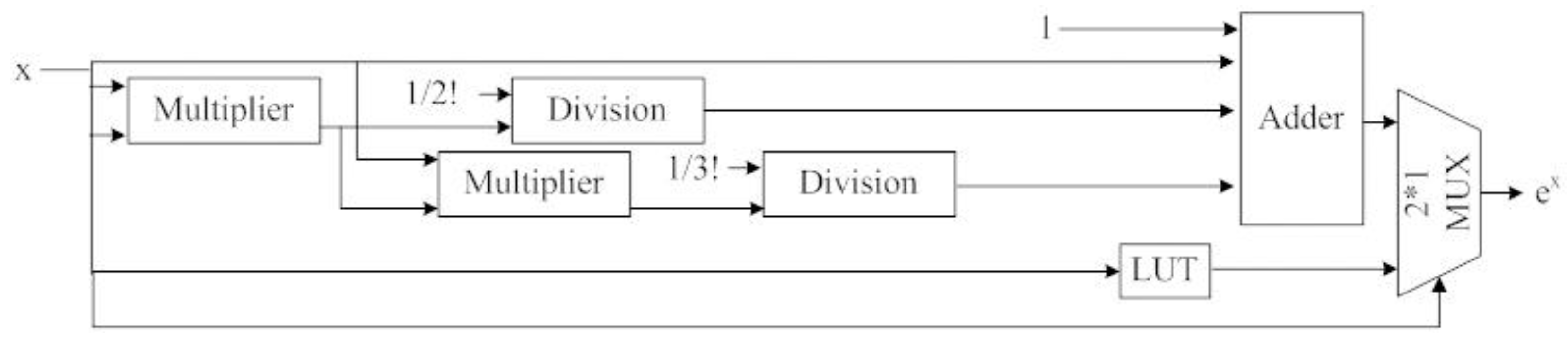
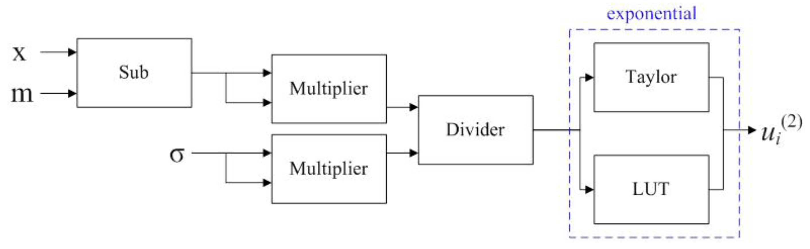
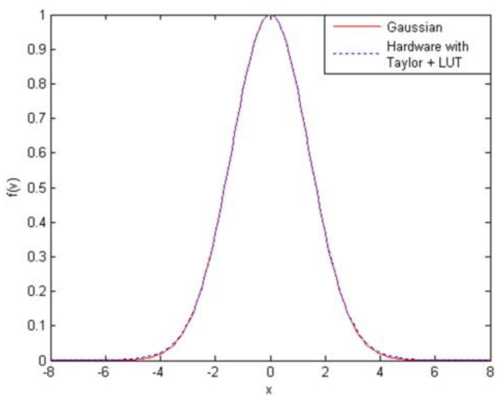
5.2.1. Gaussian Function Implementation

According to the operation of exponential function in Gaussian function, we utilized the Taylor expansion to implement the exponential function in FPGA. This way, we could implement the hardware, which spends reasonable gate counts. We used the multiplier operation to make x² and x³ two values, and divided these values by 2!, and 3!, respectively. In the Taylor expansion, 1, 1!, 2!, and 3! are four constant regular values, so we undertook the operation of these four values at the beginning, and then put them into the Gaussian function circuit of the FPGA. Finally, we used an adder tree to obtain a similar result of the Taylor expansion. In Figure 5, the block diagram shows the implementation of the exponential function. The hardware implementation of the Gaussian function in layer 2 of the TSK-type fuzzy model is shown in Figure 6. Figure 7 shows the Gaussian function and its Taylor approximation. In the range of operation, the outputting value of Gaussian function can approach the amount outcomes of software in FPGA. However, the input values are not accurate in the Taylor expansion. The input value is either a large positive value or a large negative value. According to the aforementioned problem, the LUT was utilized to compensate for the error. Therefore, regardless of whether the input shows a large positive value or a large negative value, the LUT supported the values to the multiplexer automatically. In Figure 8, we can see that the block diagram shows the implementation of the exponential function with the Taylor expansion and LUT. The block diagram is the implementation of Gaussian function with Taylor expansion and LUT as shown in Figure 9. In Figure 10, the Gaussian function is compared with its Taylor expansion and LUT approximation. Comparing Figure 7 with Figure 10, we can see that the Gaussian function approximate was more accurate than using the Taylor expansion and LUT.

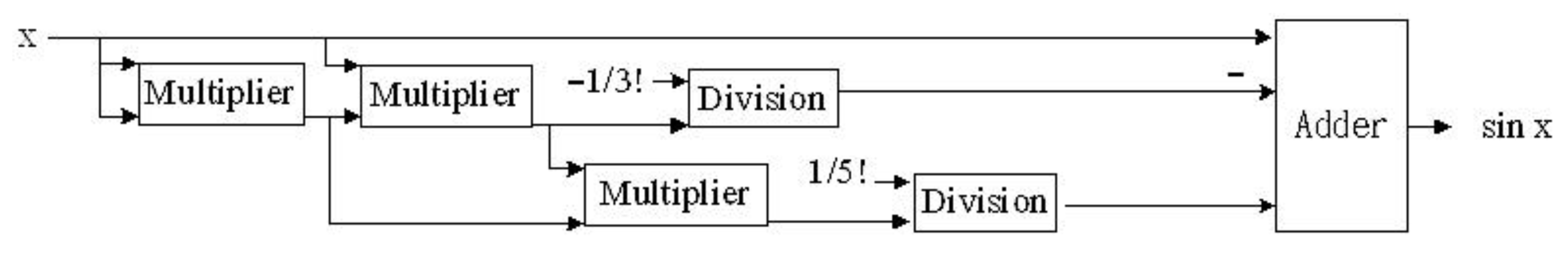
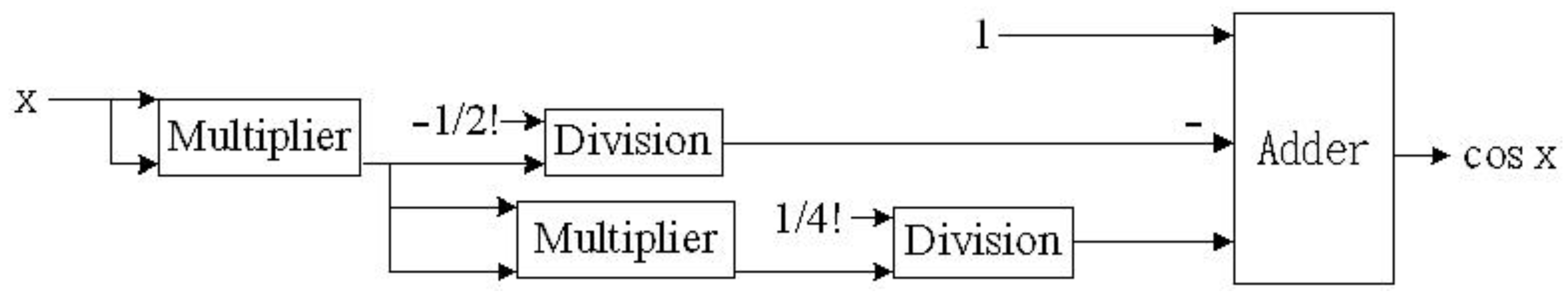
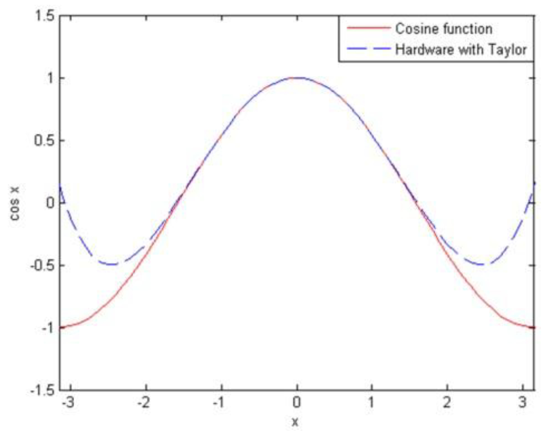
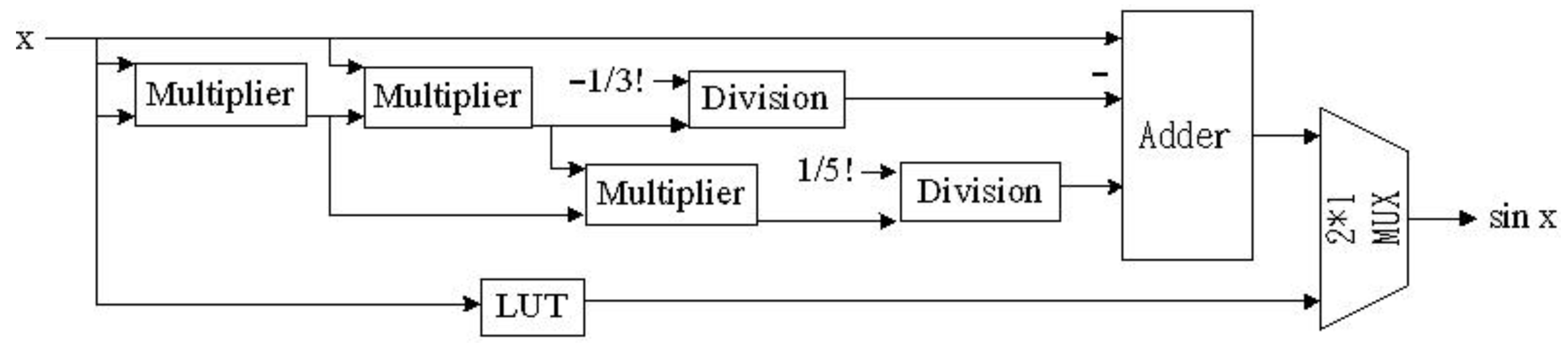
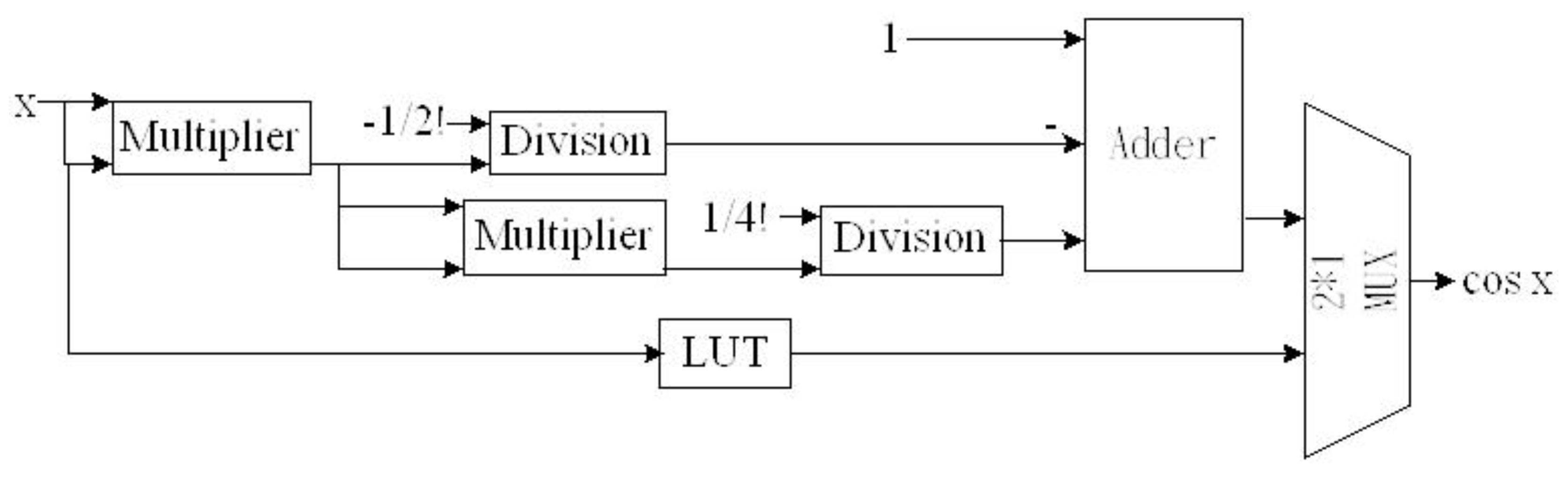
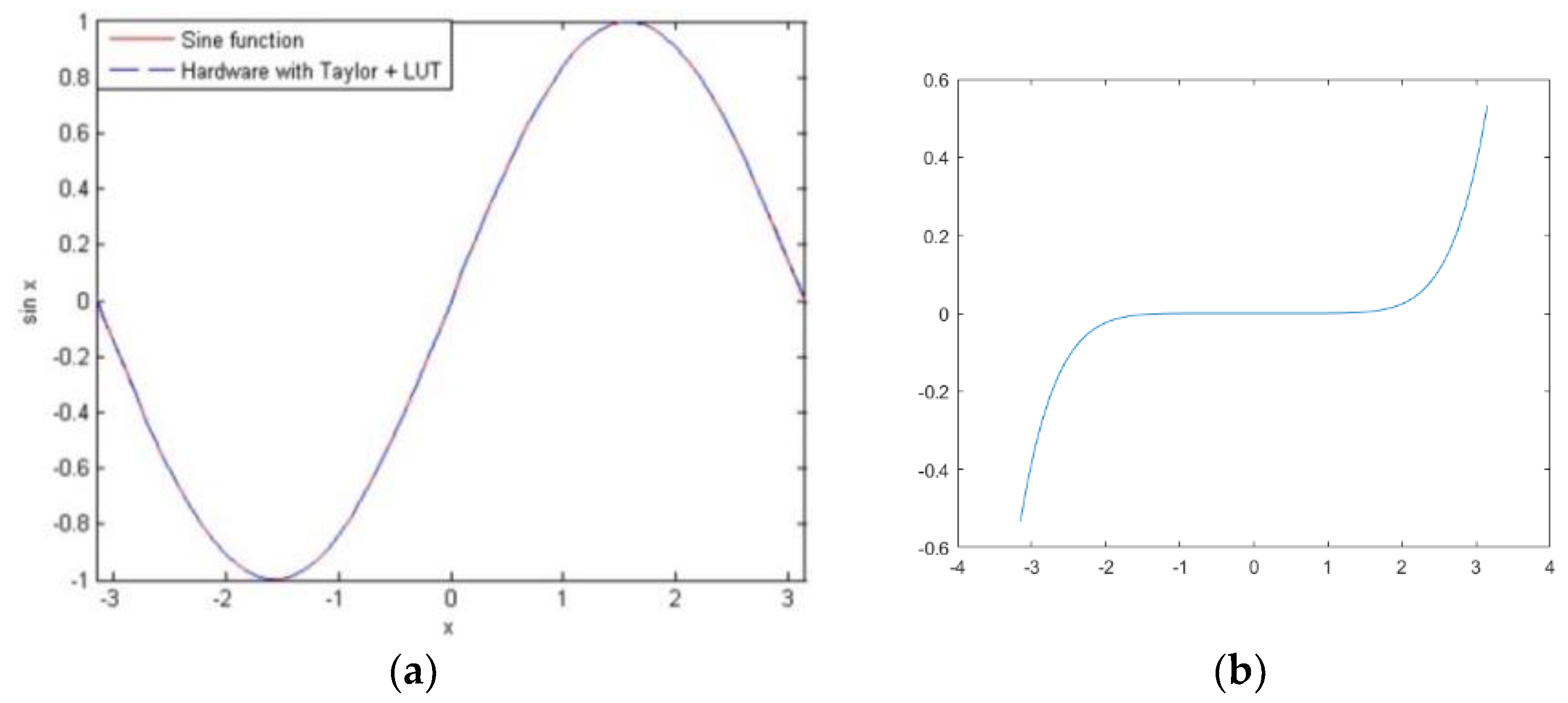
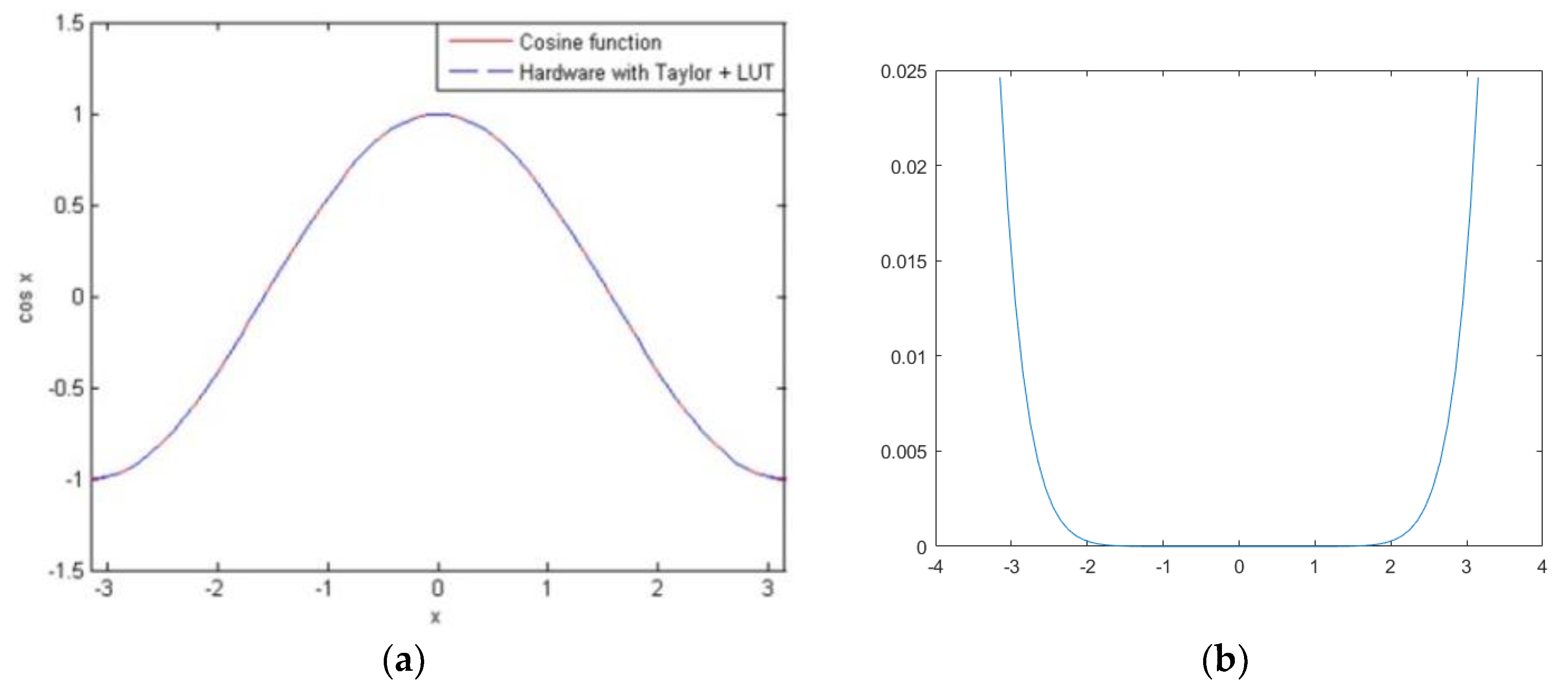
5.2.2. Sine Function and Cosine Function Implementation

Based on the operation of sine and cosine functions, the same method of the Taylor expansion was utilized to implementation sine and cosine functions in FPGA. Figure 11 and Figure 12 show the implementation of sine and cosine functions with Taylor expansion. Figure 13 and Figure 14 show the results of cosine function and sine function by the Taylor approximation. In the range of operation, the output value of the cosine function and sine function could approach the outcome of software in FPGA. However, some accurate values in the Taylor expansion will occur, such as a large positive or negative input. According to the aforementioned problem, we utilized the LUT to compensate for this error. Therefore, if the input had a large positive or negative value, the LUT will automatically support the values to the multiplexer. Figure 15 and Figure 16 show the implementation of the cosine and sine functions with the Taylor expansion and LUT. In Figure 17a and Figure 18a, the cosine function and sine function approach was more accurate by using the Taylor expansion and LUT. Figure 17b and Figure 18b show the error rate and the MSE used to estimate the error rate. The MSE of the Taylor and LUT approximation of the sine function and cosine function were equal to 0.00003922 and 0.00041378, respectively.

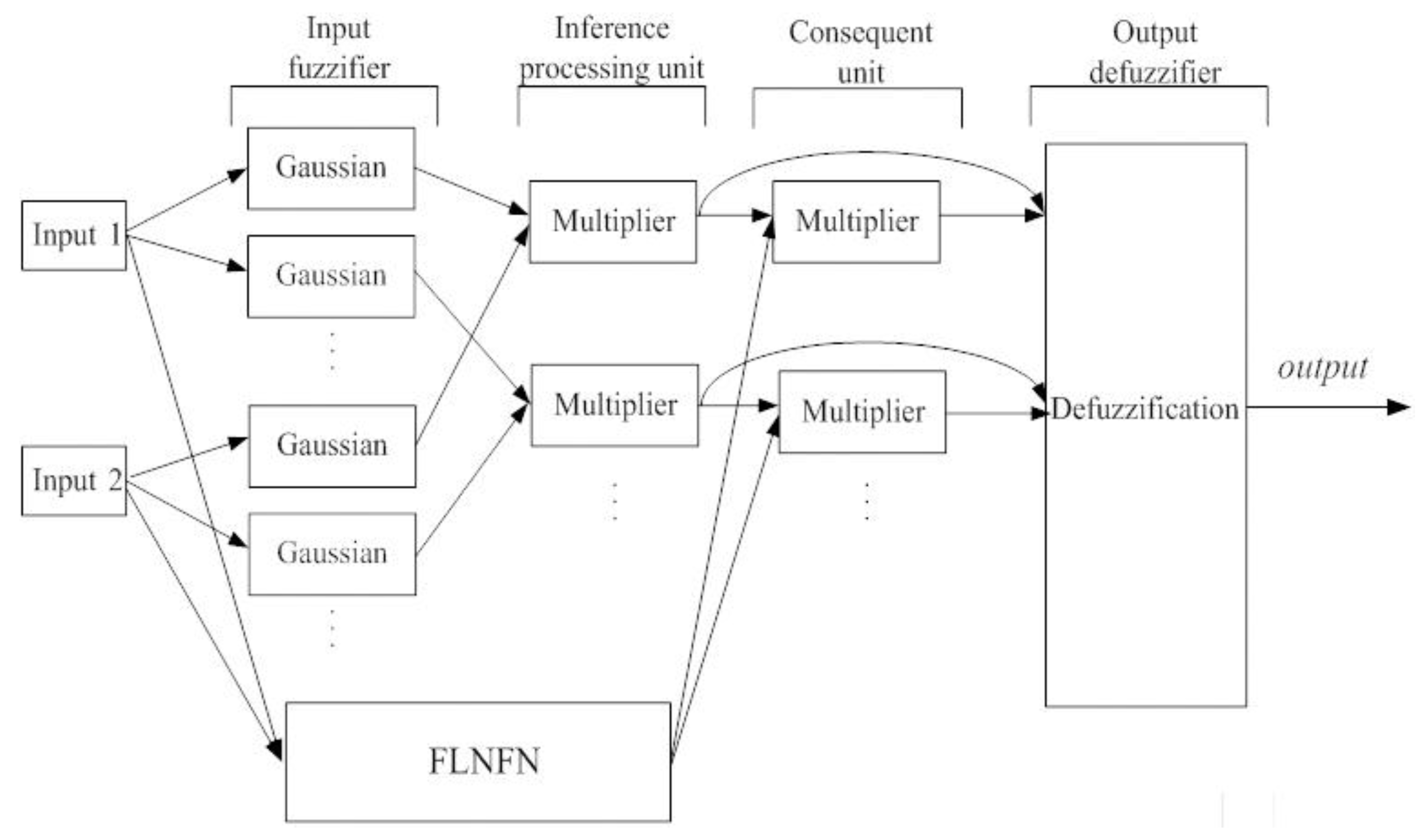
5.3. Hardware Implementation of FNFN Controller

5.3.1. Input Fuzzifier

The fuzzification operator is implemented in Equation (3). The Gaussian function in this module is the main structure of the fuzzy rules in the FNFN. The implementation of the Gaussian membership function in Equation (3) is complex by the conventional active functions. Therefore, the Taylor expansion and LUT were used to approach the Gaussian membership function. A detailed description is given in Section 5.2.1. In Section 5.2.1, Figure 9 shows the block diagram of the Gaussian function with Taylor expansion and LUT. Four multipliers, a subtracter, three dividers, a multiplexer, and an adder were used. In all of the components, the multiplier and divider were the main parts of the hardware implementation.

5.3.2. Inference Processing Unit

The multiplication operation in Equation (4) was performed in the inference processing unit. Figure 19 shows the block diagram of the inference processing unit.

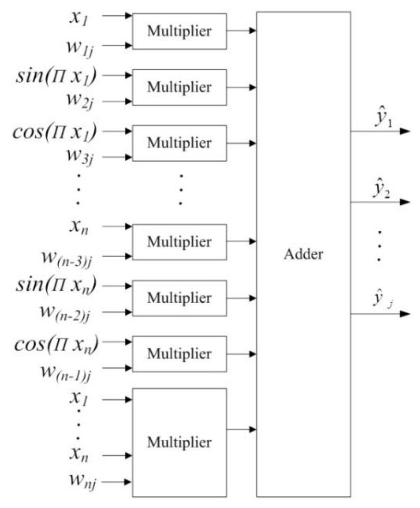
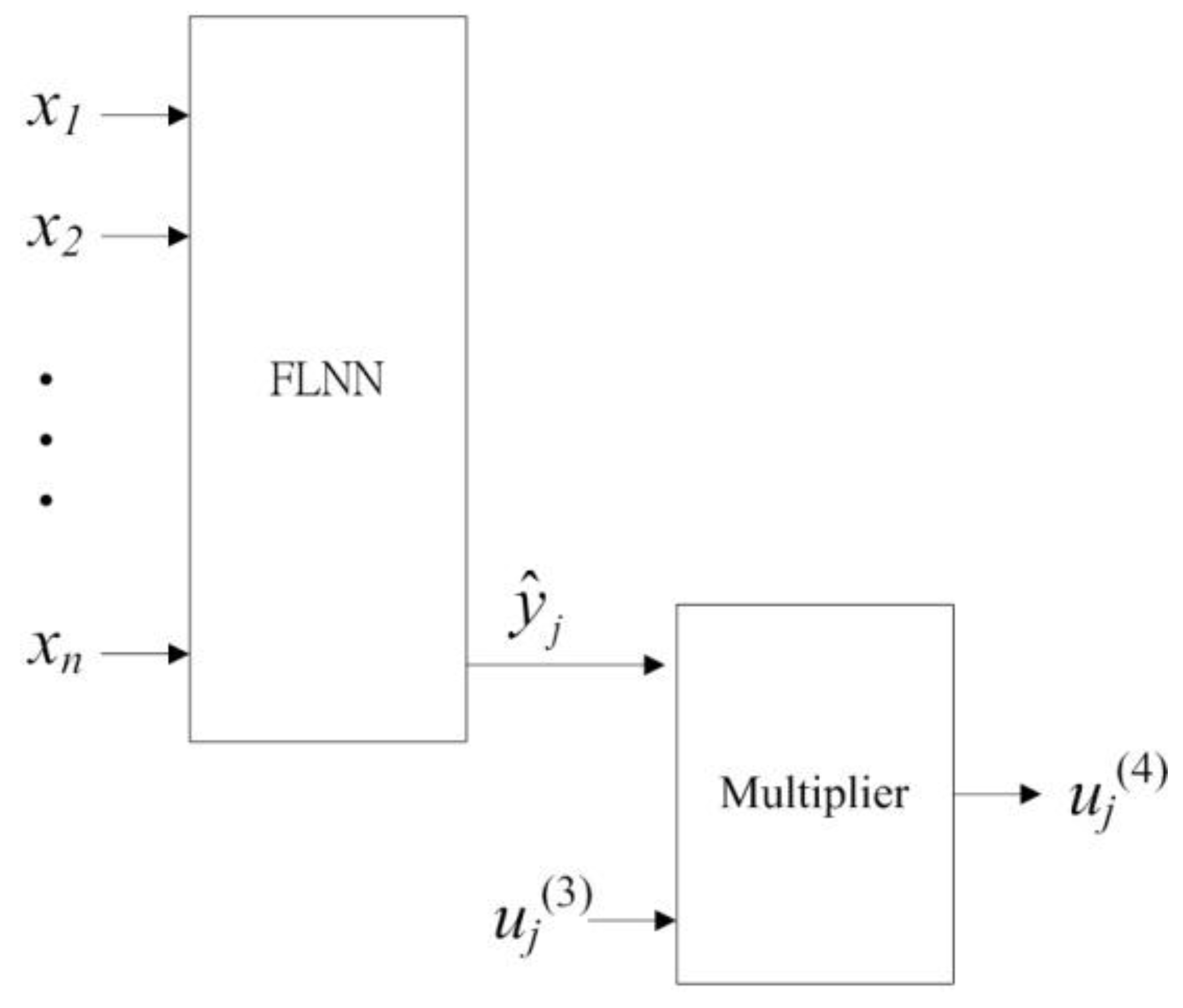
5.3.3. Consequence Unit

The main work of the consequence unit is to carry out the operation of consequence nodes in Equation (5). In layer 4, the nodes of this layer represent the consequent nodes. The inputs of layer 4 are the outputs of a FLNN and layer 3. The consequence unit module is built by multipliers and FLNN and is illustrated in Figure 20. Figure 4 presents the hardware architecture of FLNN.

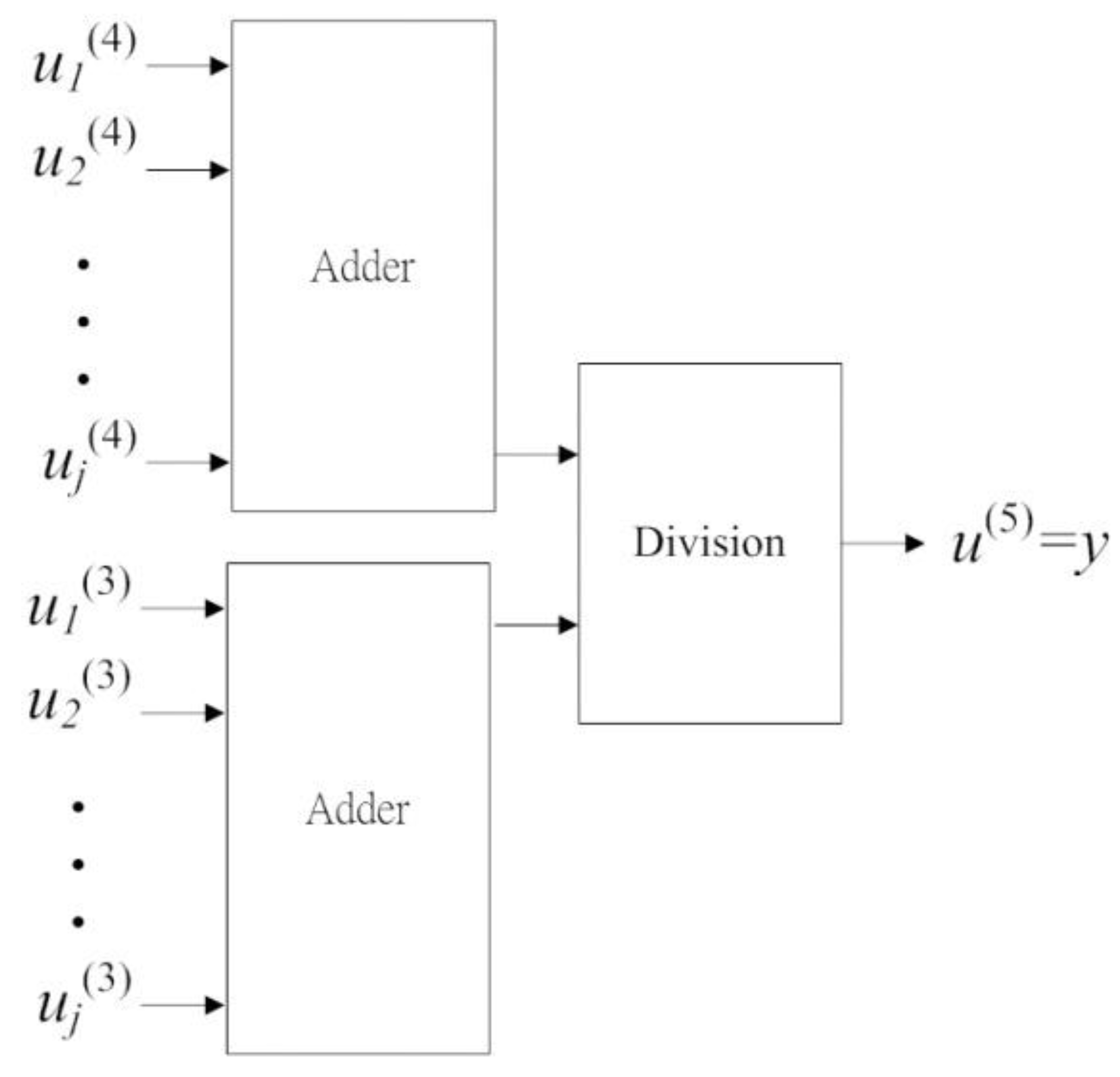
5.3.4. Output Defuzzifier

This module implements Equation (6) and the block diagram is shown in Figure 21. First, the signal $u_j^{(3)}$ and signal $u_j^{(4)}$ adopted the adder operation to sum all the values, respectively. After being added, the sum of $u_j^{(4)}$ value was divided by the sum of the $u_j^{(3)}$ value.

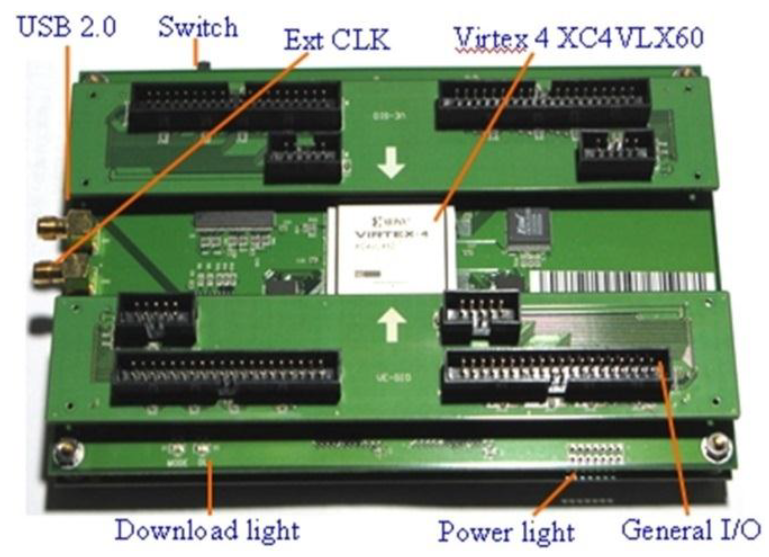
5.4. FPGA Development Platform

The hardware implementation of a FNFN controller was built in SMIMS VeriEnterprise^®. Figure 22 shows the SMIMS VeriEnterprise^® FPGA development platform with a Xilinx Virtex 4–XC4VLX60 chip. This development platform is a high-speed PC-based FPGA platform. The key features of the platform are: (1) On-board 128 MB DDR; (2) data transfer with USB 2.0 interface; (3) On-board 16 MB Flash; (4) Up to 168 additional available I/Os; (5) two independent banks—on-board 16 MB Pseudo SRAMs; (6) Download FPGA configuration through USB; (7) Two External Clock SMA Connector; and (8) Maximum data transmit rate between PC and FPGA was 211 Mbps [12].

6. Experimental Results

To verify the control performance of the FNFN, two control problems were tested in the experiments. The FNFN controller was used for solving the temperature control of a water bath [11] and the backing control of a car [22]. The design of the FNFN controller was programmed by ISE 9.1i software and used MATLAB 7.0 software for the example. The FNFN controller as implemented in the SMIMS VeriEnterprise^® FPGA development platform with a Xilinx Virtex 4–XC4VLX60 chip [12], and its clock rate was set to 50 MHz for the two examples.

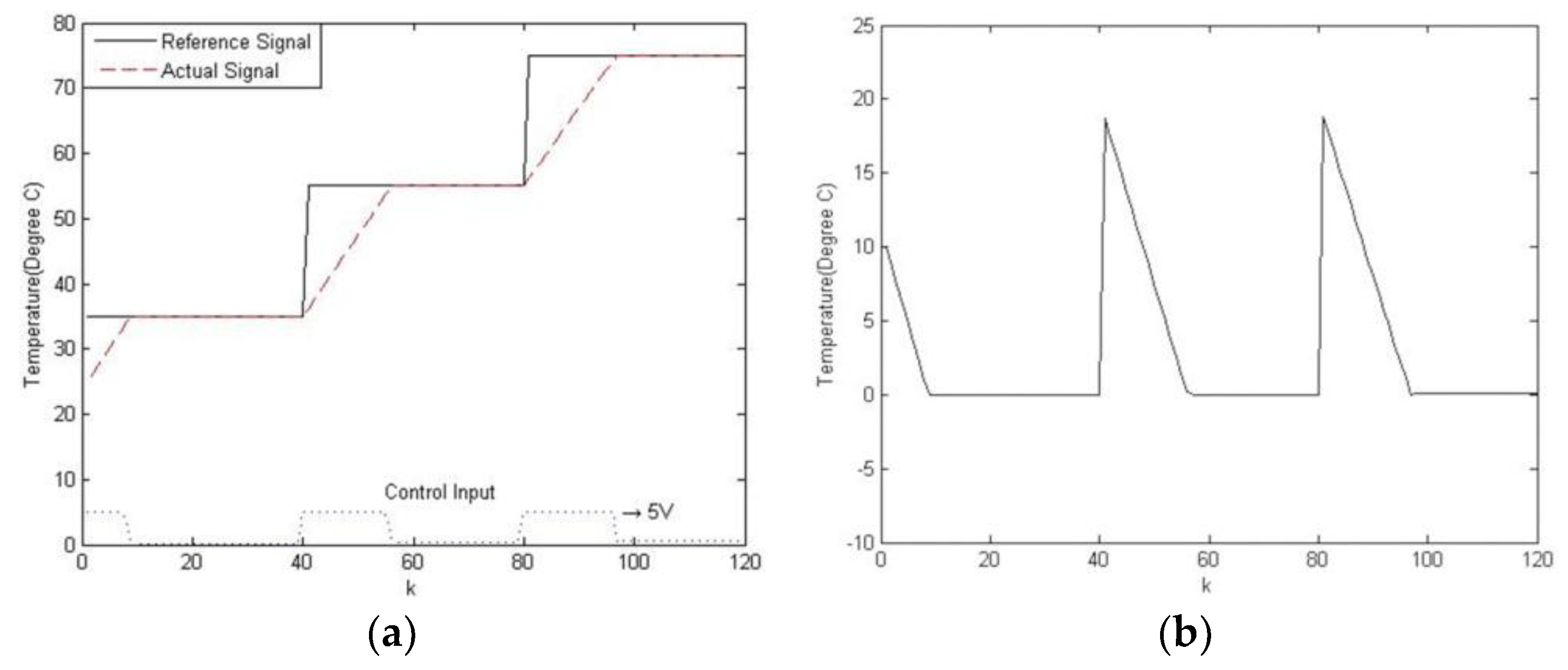
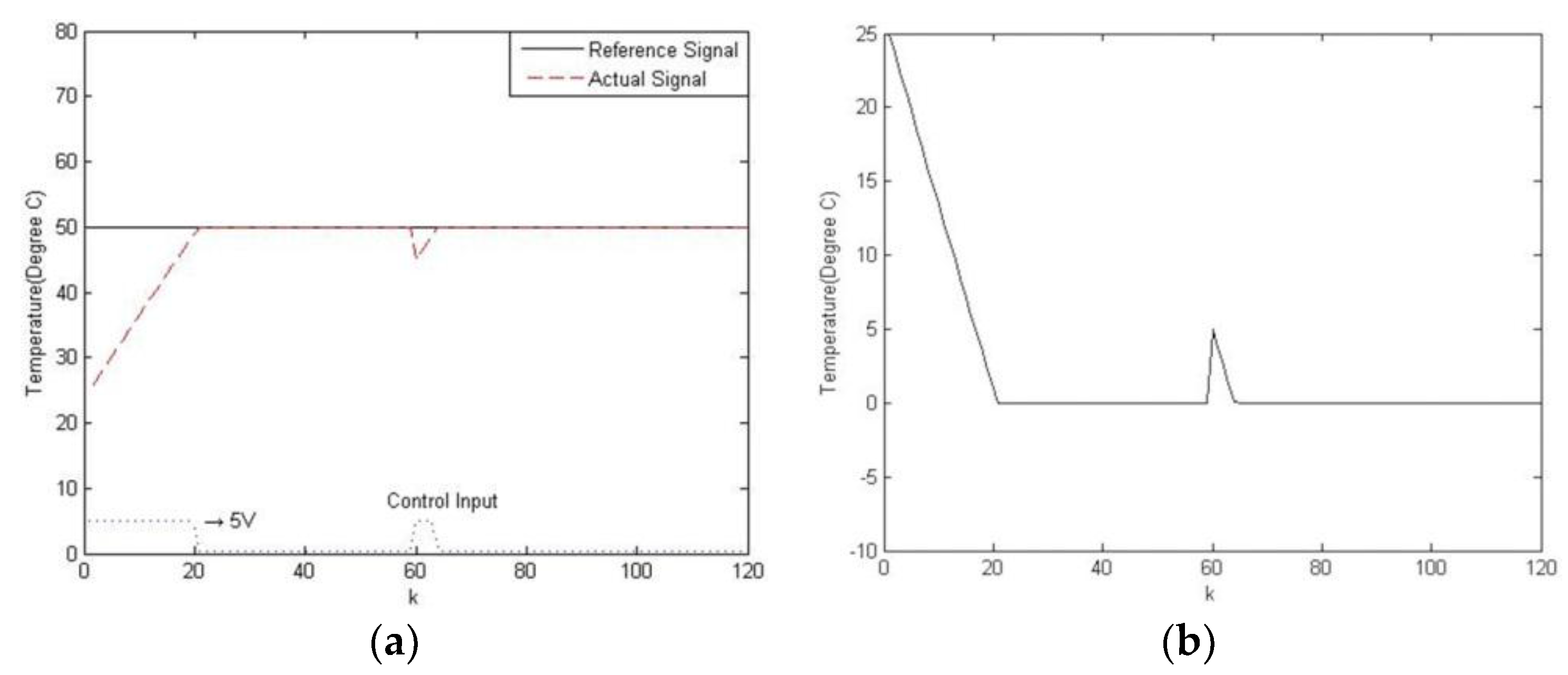
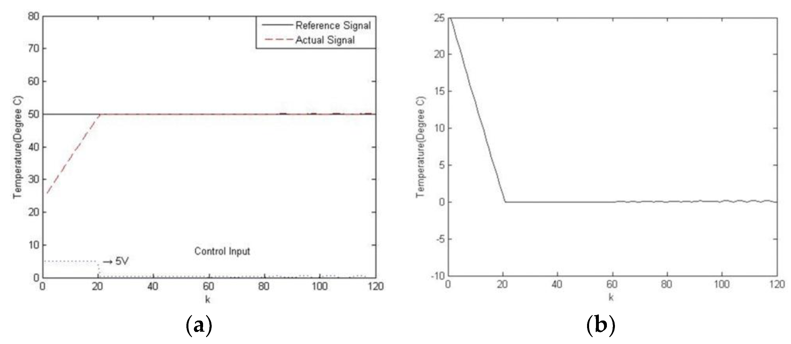
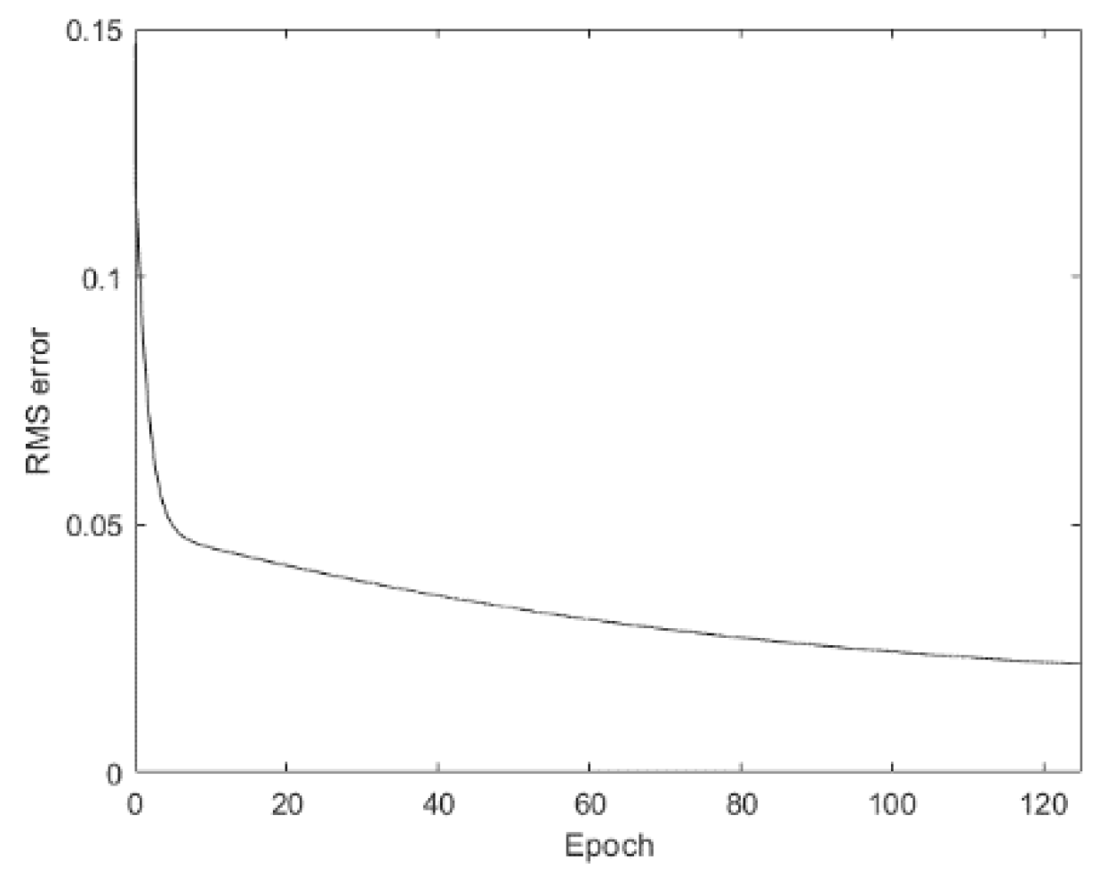
6.1. Temperature Control of a Water Bath

The objective of this experiment was to implement the temperature control of a water bath by the FNFN. The dynamic equation of a water bath is described as follows:

$$y(k+1)=e^{-\alpha Ts}y(k)+\frac{\frac{\delta }{\alpha }\left(1-e^{-\alpha Ts}\right)}{1+e^{0.5y(k)-40}}u(k)+\left[1-e^{-\alpha Ts}\right]y_0$$

(22)

where k is the discrete-time index; u(k) and y(k) denote the system input and output, respectively; and Ts is the sampling period. α and δ are constant values.

In this experiment, the parameters of the water bath plan were δ = 8.67973 × 10⁻³, α = 1.0015 × 10⁻⁴, and y₀ = 25.0 (°C), which were obtained from a real water bath plant [11]. The input u(k) was limited to 0, and 5 V represents the voltage unit. The sampling period was Ts = 30.

A schematic diagram of the temperature control of the water bath is shown in Figure 23. This program has two processes: The training process and the control process. In the training process, switches S1 and S2 were connected to nodes 1 and 2, respectively, to form a training loop. In this loop, the training data with input vector I(k) = [y_P(k + 1)y_P(k)] and desired output u(k) were defined, where the inputs of the FNFN controller were the same as that used in the inverse modeling [13]. In the control process, switches S1 and S2 were connected to nodes 3 and 4, respectively, to form a control loop. In this loop, the control signal $\widehat{u}(k)$ was generated according to the input vector I’(k) = [y_ref(k + 1)y_P(k)], where y_P is the plant output and y_ref is the reference model output.

The random input signals u_rd(k) were constrained between [0, 5] V and infused directly into the dynamic equation of the water bath as described in Equation (22). Based on the input–output characteristics to cover the entire reference output, 120 training patterns were selected. The initial water temperature was set to 25 °C. When a random input signal was infused, the temperature of the water rose progressively. After 15,000 training iterations, four fuzzy rules were generated. The obtained fuzzy rules in FNFN are as follows.

Rule 1:

$$\begin{array}{l}IF{x}_{1}is\mu \left(0.995031,0.91\right)and{x}_{2}is\mu \left(0.988214,0.084\right)\\ THEN{\widehat{y}}_1=23.753880x_1-20.0154785\sin \left(\pi x_1\right)-11.353351\cos \left(\pi x_1\right)\\ -23.073202x_2+18.681133\sin \left(\pi x_2\right)+15.328705\cos \left(\pi x_2\right)\\ +3.764496x_1{x}_2\end{array}$$

Rule 2:

$$\begin{array}{l}IF{x}_{1}is\mu \left(0.997067,0.84\right)and{x}_{2}is\mu \left(0.998780,0.35\right)\\ THEN{\widehat{y}}_2=6.520161x_1-21.382976\sin \left(\pi x_1\right)-1.787920\cos \left(\pi x_1\right)\\ -6.960691x_2+21.554704\sin \left(\pi x_2\right)+2.924881\cos \left(\pi x_2\right)\\ +0.238945x_1{x}_2\end{array}$$

Rule 3:

$$\begin{array}{l}IF{x}_{1}is\mu \left(0.818868,0.47\right)and{x}_{2}is\mu \left(0.141187,0.62\right)\\ THEN{\widehat{y}}_3=-0.602595x_1+0.207561\sin \left(\pi x_1\right)-0.455584\cos \left(\pi x_1\right)\\ -0.602411x_2-0.969473\sin \left(\pi x_2\right)+0.493613\cos \left(\pi x_2\right)\\ -0.109840x_1{x}_2\end{array}$$

Rule 4:

$$\begin{array}{l}IF{x}_{1}is\mu \left(0.002391,0.082\right)and{x}_{2}is\mu \left(0.000861,0.92\right)\\ THEN{\widehat{y}}_4=20.333939x_1-5.231502\sin \left(\pi x_1\right)-10.808845\cos \left(\pi x_1\right)\\ -19.797790x_2-5.819267\sin \left(\pi x_2\right)+10.899276\cos \left(\pi x_2\right)\\ +1.701125x_1{x}_2\end{array}$$

In this study, we compared the control performance of the proposed FNFN with those of the Takagi–Sugeno–Kang (TSK)-type neural fuzzy network (NFN) [2], the functional link neural network (FLNN) [4], the proportional–integral–derivative (PID) controller [23], and the manually designed fuzzy controller [24]. The performance evaluation consisted of the regulation of set-points, the noise influence, and the tracking capability.

The first work was to evaluate the regulation of three points.

$$y_{ref}\left(k\right)=\{\begin{array}{c}{35}^o,ifk\le 40\\ {55}^o,if40<k\le 80\\ {75}^o,if80<k\le 120\end{array}$$

(23)

The results of the regulation of the set-points using the FNFN controller are shown in Figure 24a. Figure 24b illustrates the errors between the FNFN output and desired output. The performance evaluation adopted the sum of absolute error (E) and is described as follows:

$$E={\displaystyle \sum }_k\left|y_{ref}\left(k\right)-y\left(k\right)\right|$$

(24)

where y(k) and y_ref(k) are the actual output and desired output, respectively.

The second experiment was to obtain the noise influence of the FNFN controller. At the 60th sampling time, a noise value was added to the output of the water bath system (i.e., −5 °C). This experiment adopted a pre-set temperature of 50 °C. For the noise influence, the outputs and the corresponding errors of the FNFN controller are presented in Figure 25a,b, respectively. After the occurrence of the noise influence, the proposed FNFN controller had a very quick and steady recovery.

The parameters of many industrial-control processes will be altered in an irregular way. The third experiment was to add a 0.7 × u(k−2) value to the input of the water bath system after the 60th sampling time for testing the robustness of the FNFN controller. This experiment adopted a pre-set temperature (i.e., 50 °C). When the plant dynamics were altered, the outputs and the corresponding errors of the FNFN controller are shown in Figure 26a,b, respectively. The training process continued for 125 epochs. Figure 27 shows the learning curve of the FNFN controller in the water bath system.

In the final experiment, the tracking capability of the proposed FNFN was proven. The ramp-reference signals are defined as follows:

$$y_{ref}\left(k\right)=\{\begin{array}{c}\begin{array}{c}{34}^o,ifk\le 30\\ {(0.5k+19)}^o,if30<k\le 50\end{array}\\ \begin{array}{c}{(0.8k+4)}^o,if50<k\le 70\\ \begin{array}{c}{(25+0.5k)}^o,if70<k\le 90\\ {70}^o,if90<k\le 120\end{array}\end{array}\end{array}$$

(25)

The tracking outputs and the errors of the FNFN controller are shown in Figure 28a,b, respectively.

The sums of the absolute error (E) of the FNFN controller with software implementation and with hardware implementation, the Takagi–Sugeno–Kang (TSK)-type neural fuzzy network (NFN) [2], the functional link neural network (FLNN) [4], the proportional–integral–derivative (PID) controller [23], and the manually designed fuzzy controller [24] are shown in

Table 2. Results of the comparison of various controllers.

E	FNFN Controller		TSK-Type NFN Controller [2]	FLNN Controller [4]	PID Controller [23]	Fuzzy Controller [24]
	Software	Hardware
Regulation	353.13	354.49	361.96	379.22	418.5	401.5
Noise Influence	270.72	271.59	274.75	324.51	311.5	275.8
Plant Dynamics Altered	263.68	264.57	265.48	311.54	322.2	273.5
Tracking	44.53	46.48	54.28	98.43	100.6	88.1

. The experimental results showed that the trained FNFN controller had better noise rejection capabilities and tracking control performance than the other methods in the temperature control of the water bath.

The hardware implementation of the FNFN with four fuzzy logic rules needed to use about 507,064 logic gates. The resource requirements for the example architecture with FNFN implementation are shown in

Table 3. Resources requirements of FNFN implementation for the temperature control.

Device Selected	XC4VLX60
Logic Gate Utilization	Available	Used	Utilization
Slices	26,624	26,352	98%
4 input LUTs	53,248	50,117	94%
Slice Flip Flops	53,248	50,607	9%
GCLKs	32	1	3%
Bonded IOBs	640	61	9%
Gate counts	6,000,000	507,064	8.5%

. In this table, “Available” represents the various resources of the chip present; “Used” represents the resources utilized in our implementation, and “Utilization” represents the percentage of resources utilized. Experimental results showed that the proposed method obtained perfect control capability.

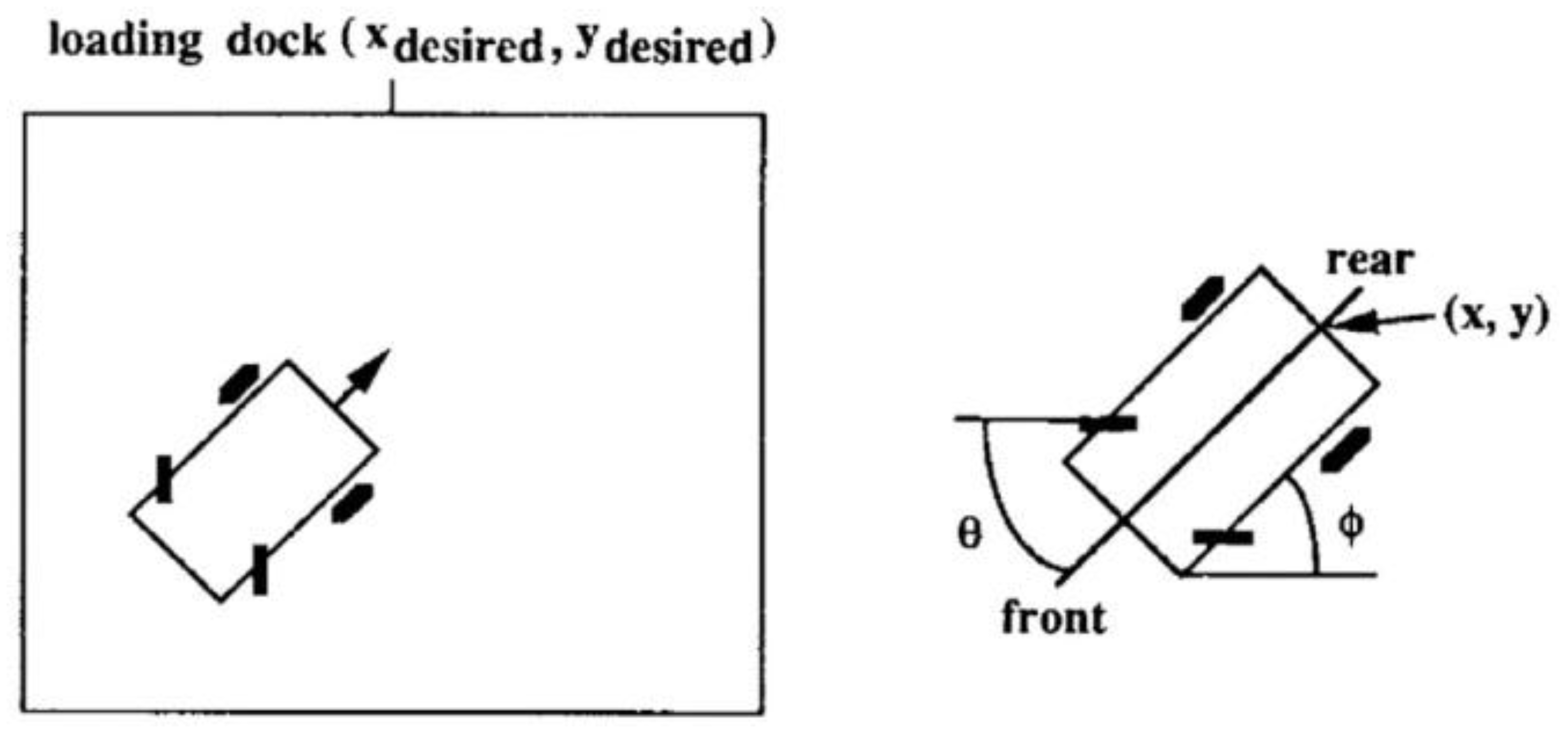
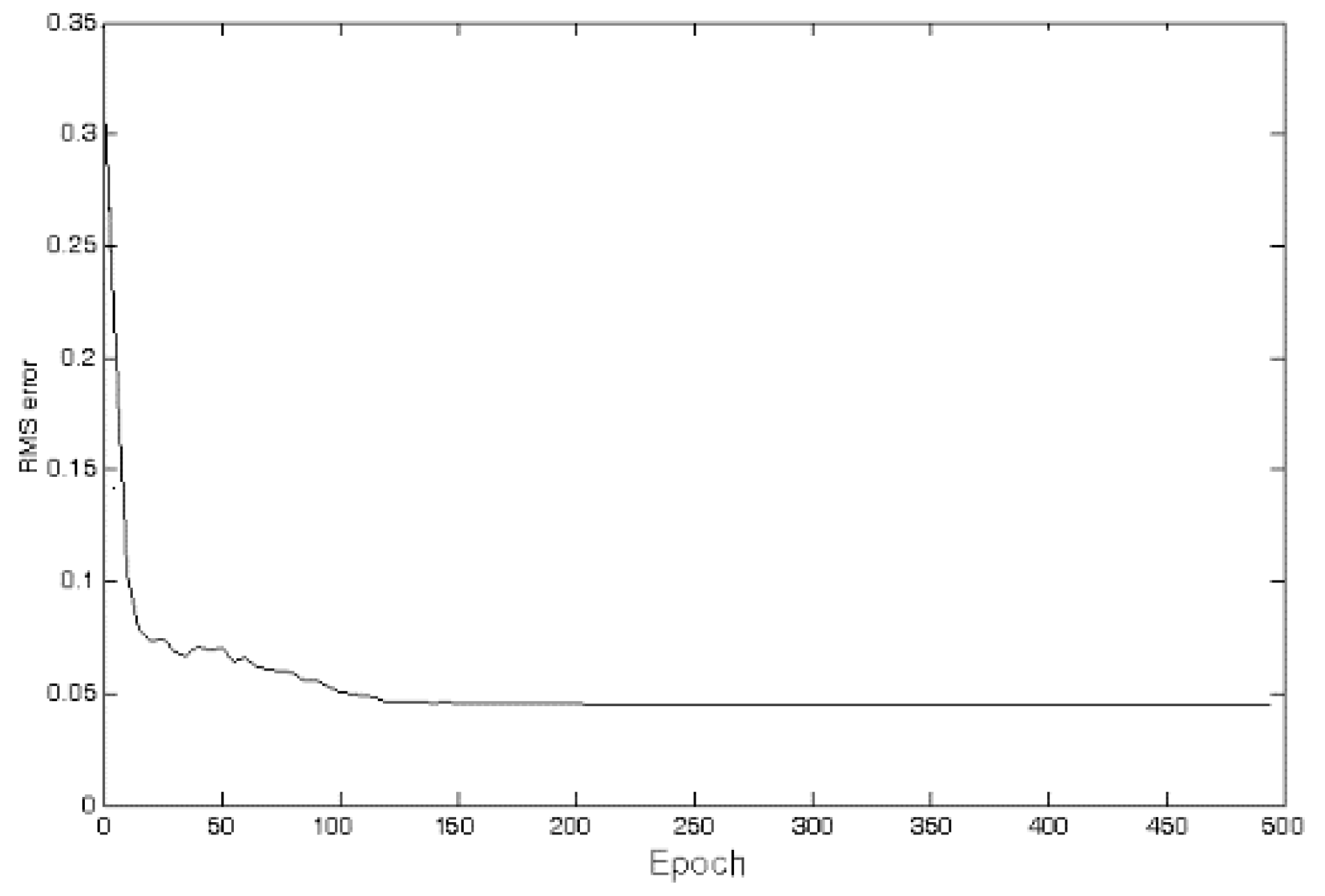
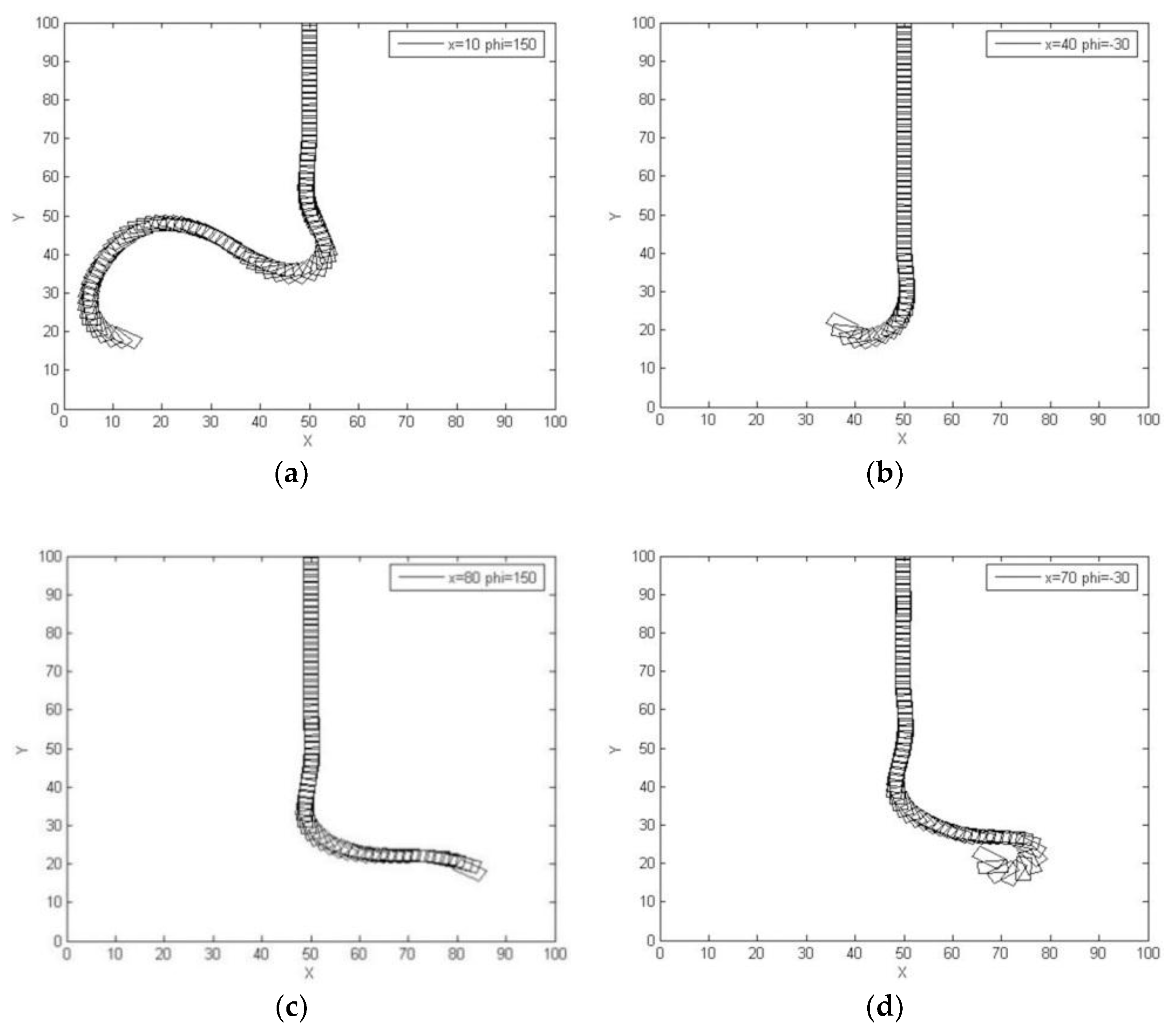
6.2. Backing Control of a Car

As the backing control of a car is a complex control problem, the traditional control method is difficult to implement [22]. The loading zone and car are presented in Figure 29. The φ, x, and y variables were used to decide the car position. The (x, y) denotes the center position of the car and φ presents the angle between the horizontal axis and the car. The steering angle of the car (θ) is the controlled variable. The objective of this control was to move the car to the desired dock (x_desired, y_desired) at φ_desired = 90°. A fixed distance (d_b) of the car was moved backwards at each time step. The plane [0, 100] × [0, 100] represents the limited loading region.

The angle φ and cross position x of the car are two inputs of the proposed FNFN, whereas the steering angle θ presents the output of the proposed FNFN. The ranges of parameters (x, $\varnothing$, and θ) are described as follows.

$$0\le x\le 100$$

(26)

$$-90°\le \varphi \le 270°$$

(27)

$$-30°\le \theta \le 30°$$

(28)

The dynamical equations of the car are

$$\begin{array}{c}x\left(k+1\right)=x\left(k\right)+cos\varnothing \left(k\right)+d_{b}cos\theta \left(k\right)\\ y\left(k+1\right)=y\left(k\right)+sin\varnothing \left(k\right)+d_{b}cos\theta \left(k\right)\\ \varnothing \left(k+1\right)=ta{n}^{-1}\left[\frac{d_{l}sin\varnothing \left(k\right)+d_{b}cos\varnothing \left(k\right)sin\theta \left(k\right)}{d_{l}cos\varnothing \left(k\right)-d_{b}cos\varnothing \left(k\right)sin\theta \left(k\right)}\right]\end{array}$$

(29)

where d_l denotes the car length.

After BP training processing, four fuzzy rules were generated and the parameters of the membership functions also determined in the FNFN controller. Therefore, the total number of adjustable parameters was 44. The training process continued for 500 iterations. The RMS errors of the FNFN were approximately 0.0329. There were four fuzzy rules generated, which are shown as follows.

Rule 1:

$$\begin{array}{l}IF{x}_{1}is\mu \left(2.46678,0.64\right)and{x}_{2}is\mu \left(0.180007,0.71\right)\\ THEN{\widehat{y}}_1=0.500968x_1-0.818936\sin \left(\pi x_1\right)+1.77709\cos \left(\pi x_1\right)\\ -2.76852x_2+0.722349\sin \left(\pi x_2\right)-1.0599\cos \left(\pi x_2\right)\\ +4.02142x_1{x}_2\end{array}$$

(30)

Rule 2:

$$\begin{array}{l}IF{x}_{1}is\mu \left(-0.53439,0.2\right)and{x}_{2}is\mu \left(-0.294915,0.64\right)\\ THEN{\widehat{y}}_2=-0.943522x_1+0.884788\sin \left(\pi x_1\right)-0.196846\cos \left(\pi x_1\right)\\ +0.713501x_2-1.1581\sin \left(\pi x_2\right)-0.162965\cos \left(\pi x_2\right)\\ -7.97909x_1{x}_2\end{array}$$

(31)

Rule 3:

$$\begin{array}{l}IF{x}_{1}is\mu \left(-11.8231,0.98\right)and{x}_{2}is\mu \left(4.34674,0.81\right)\\ THEN{\widehat{y}}_3=2.58614x_1-0.570534\sin \left(\pi x_1\right)-2.00722\cos \left(\pi x_1\right)\\ +1.61986x_2+1.46359\sin \left(\pi x_2\right)-2.69316\cos \left(\pi x_2\right)\\ +0.0618043x_1{x}_2\end{array}$$

(32)

Rule 4:

$$\begin{array}{l}IF{x}_{1}is\mu \left(-0.840175,0.52\right)and{x}_{2}is\mu \left(-1.11993,0.74\right)\\ THEN{\widehat{y}}_4=1.46606x_1+1.14098\sin \left(\pi x_1\right)-0.75915\cos \left(\pi x_1\right)\\ +1.07353x_2+0.74087\sin \left(\pi x_2\right)+3.4868\cos \left(\pi x_2\right)\\ -1.73986x_1{x}_2\end{array}$$

(33)

Figure 30 presents the FNFN controller learning curve and Figure 31a–d show the moving car trajectories of the trained FNFN controller with the four different initial positions. The RMSE is adopted to evaluate the FNFN performance;

Table 4. The RMSE of a car backing control.

Position	E
(a)	0.2691
(b)	0.1519
(c)	0.1955
(d)	0.2454

shows the RMSE of the four different initial positions. Experimental results showed that the trained FNFN could be successfully reloaded from different initial positions.

The hardware implementation of the FNFN with four fuzzy logic rules needed to use about 507,064 logic gates.

Table 5. Resource requirements of FNFN implementation the backing control of a car.

Device Selected	XC4VLX60
Logic Gate Utilization	Available	Used	Utilization
Slices	26,624	26,352	98%
4 input LUTs	53,248	50,117	94%
Slice Flip Flops	53,248	50,607	9%
GCLKs	32	1	3%
Bonded IOBs	640	61	9%
Gate counts	6,000,000	507,064	8.5%

illustrates the resource requirements for the control architecture of backing up the truck with FNFN implementation. In this table, “Available” represents the various resources of the chip present; “Used” represents the resources utilized in our implementation, and “Utilization” represents the percentage of resources utilize. Experimental results showed that the proposed method obtained perfect control capability.

7. Conclusions and Future Works

This study presented the hardware implementations of FNFN using Xilinx FPGAs for solving nonlinear control problems. The proposed FNFN uses a functional link neural network as the conclusion part of a fuzzy rule, which has a nonlinear combination of inputs. In addition, an efficient learning algorithm was proposed to construct the architecture of the FNFN using structure learning, and adjust the parameters using parameter learning. The main advantage of the FNFN is a reduced computational cost in the training stage, while maintaining the approximation performance of the multi-layer perceptron network. However, FNFN has the disadvantage of an increased number of rules as it cannot automatically generate the optimum rule numbers and merge similar rules. In order to have high speed processing and real-time operating capability, using hardware implementation is necessary.

To evaluate the control performance of the proposed FNFN, two experiments including the temperature control of a water bath and the backing control of a car were performed. Finally, the performances of the experimental results successfully confirmed the validity of using FPGA implementation for the FNFN controller. In future work, we will decrease the resource requirements for designing the model and implement the learning algorithm in FPGA. In addition, a type-2 fuzzy set incorporates uncertainty about the membership function into fuzzy set theory. Many reported results have shown that the type-2 neural fuzzy network is better able to handle uncertainties than the type-1 neural fuzzy network. In future work, we will consider type-2 fuzzy sets to improve the structure of the type-1 neural fuzzy network and implement this using hardware.

References

1. Wang, J.G.; Tai, S.C.; Lin, C.J. The application of an interactively recurrent self-evolving fuzzy CMAC classifier on face detection in color images. Neural Comput. Appl. 2018, 29, 201–213. [Google Scholar] [CrossRef]
2. Jang, J.-S.R. ANFIS: Adaptive-network-based fuzzy inference system. IEEE Trans. Syst. Man Cybern. 1993, 23, 665–685. [Google Scholar] [CrossRef]
3. Wu, M.F.; Huang, W.C.; Juang, C.F.; Chang, K.M.; Wen, C.Y.; Chen, Y.H.; Lin, C.Y.; Chen, Y.C.; Lin, C.C. A new method for self-estimation of the severity of obstructive sleep apnea using easily available measurements and neural fuzzy evaluation system. IEEE J. Biomed. Health Inf. 2017, 21, 1524–1532. [Google Scholar] [CrossRef] [PubMed]
4. Lin, C.J.; Chen, C.H. Identification and prediction using recurrent compensatory neuro-fuzzy systems. Fuzzy Sets Syst. 2004, 150, 307–330. [Google Scholar] [CrossRef]
5. Khayat, O. Structural parameter tuning of the first-order derivative of an adaptive neuro-fuzzy system for chaotic function modeling. J. Int. Fuzzy Syst. 2014, 27, 235–245. [Google Scholar]
6. Ali, C.; Ambrish, C. Adaptive neuro-fuzzy based solar cell model. IET Renew. Power Gener. 2014, 8, 679–686. [Google Scholar]
7. George, S.A.; Eftychios, E.P.; Kimon, P.V. Stock trend forecasting in turbulent market periods using neuro-fuzzy systems. Oper. Res. 2016, 16, 245–269. [Google Scholar]
8. Fatemeh, Z.; Zahra, Z. A review of neuro-fuzzy systems based on intelligent control. arXiv, 2018; arXiv:1805.03138. [Google Scholar]
9. Patra, J.C.; Pal, R.N.; Chatterji, B.N.; Panda, G. Identification of nonlinear dynamic systems using functional link artificial neural networks. IEEE Trans. Syst. Man Cybern. Part B Cybern. 1999, 29, 254–262. [Google Scholar] [CrossRef] [PubMed]
10. Li, S.; Choi, K.; Lee, Y. Artificial Neural Network Implementation in FPGA: A Case Study. In Proceedings of the 2016 International Conference on SoC Design (ISOCC), Jeju, Korea, 23–26 October 2016; pp. 297–298. [Google Scholar]
11. Page, A.; Mohsenin, T. FPGA-Based Reduction Techniques for Efficient Deep Neural Network Deployment. In Proceedings of the 2016 IEEE 24th Annual International Symposium on Field-Programmable Custom Computing Machines (FCCM), Washington, DC, USA, 1–3 May 2016; p. 200. [Google Scholar]
12. Zhang, C.; Li, P.; Sun, G.; Guan, Y.; Xiao, B.; Cong, J. Optimizing FPGA-Based Accelerator Design for Deep Convolutional Neural Networks. In Proceedings of the 2015 ACM/SIGDA International Symposium on Field-Programmable Gate Arrays, Monterey, CA, USA, 22–24 February 2015; pp. 161–170. [Google Scholar]
13. Bettoni, M.; Urgese, G.; Kobayashi, Y.; Macii, E.; Acquaviva, A. A convolutional neural network fully implemented on FPGA for embedded platforms. In Proceedings of the 2017 New Generation of CAS, Genova, Genoa, 6–9 September 2017; pp. 49–52. [Google Scholar]
14. Lu, S.M.; Li, D.J. Adaptive neural network control for nonlinear hydraulic servo-system with time-varying state constraints. Complexity 2017, 2017. [Google Scholar] [CrossRef]
15. Lin, C.J.; Cheng, C.H. A recurrent neural fuzzy controller based on self-organizing improved particle swarm optimization for a magnetic levitation system. Int. J. Adapt. Control Signal Process. 2015, 29, 563–580. [Google Scholar] [CrossRef]
16. Li, S.P. Adaptive control with optimal tracking performance. Int. J. Syst. Sci. 2018, 49, 496–510. [Google Scholar] [CrossRef]
17. Gatti, C. The truck backer-upper problem. In Design of Experiments for Reinforcement Learning; Springer: Cham, Switzerland, 2015; pp. 111–127. [Google Scholar]
18. Ontiveros-Robles, E.; Vázquez, J.G.; Castro, J.R.; Castillo, O. A FPGA-Based Hardware Architecture Approach for Real-Time Fuzzy Edge Detection. In Nature-Inspired Design of Hybrid Intelligent Systems; Springer: Cham, Switzerland, 2016; pp. 519–540. [Google Scholar]
19. Aldair, A.A.; Obed, A.A.; Halihal, A.F. Design and Implementation of Neuro-Fuzzy Controller Using FPGA for Sun Tracking System. Iraqi J. Electr. Electron. Eng. 2016, 12, 123–136. [Google Scholar]
20. Kaiser, M.S.; Chowdhury, Z.I.; Al Mamun, S.; Hussain, A.; Mahmud, M. A Neuro-Fuzzy Control System Based on Feature Extraction of Surface Electromyogram Signal for Solar-Powered Wheelchair. Cogn. Comput. 2016, 8, 946–954. [Google Scholar] [CrossRef]
21. CastroCaicedo, Y.E.; Moreno, E.D.; Coelho, L.D.S.; Llanos, C.H. NeuroFuzzy Controller Design and FPGA-Based Embedded System for ACROBOT Model. Int. J. Comput. Digit. Syst. 2018, 6, 97–108. [Google Scholar] [CrossRef]
22. Lin, C.J.; Wu, C.F.; Lin, H.Y.; Yu, C.Y. An interactively recurrent functional neural fuzzy network with fuzzy differential evolution and its applications. Sains Malaysiana 2015, 44, 1721–1728. [Google Scholar]
23. Inacio, C.; Ombres, D. The DSP decision: fixed point or floating? IEEE Spectr. 1996, 33, 72–74. [Google Scholar] [CrossRef]
24. Ewe, C.T.; Cheung, P.Y.K.; Constantinides, G.A. Dual fixed-point: An efficient alternative to floating-point computation. Lect. Notes Comput. Sci. 2004, 3203, 200–208. [Google Scholar]
Figure 1. The proposed FNFN architecture.
Electronics 07 00145 g001
Figure 2. Flowchart of the proposed learning algorithm.
Electronics 07 00145 g002
Figure 3. Architecture of FNFN.
Electronics 07 00145 g003
Figure 4. Architecture of FLNN.
Electronics 07 00145 g004
Figure 5. Block diagram of exponential function with Taylor expansion.
Electronics 07 00145 g005
Figure 6. Block diagram of Gaussian function.
Electronics 07 00145 g006
Figure 7. Taylor approximation of a Gaussian function.
Electronics 07 00145 g007
Figure 8. Block diagram of exponential function with Taylor expansion and LUT.
Electronics 07 00145 g008
Figure 9. Block diagram of Gaussian function with Taylor expansion and LUT.
Electronics 07 00145 g009
Figure 10. Taylor and LUT approximation of a Gaussian function.
Electronics 07 00145 g010
Figure 11. Block diagram of the sine function with the Taylor expansion.
Electronics 07 00145 g011
Figure 12. Block diagram of the cosine function with the Taylor expansion.
Electronics 07 00145 g012
Figure 13. Taylor approximation of the sine function.
Electronics 07 00145 g013
Figure 14. Taylor approximation of the cosine function.
Electronics 07 00145 g014
Figure 15. Block diagram of the sine function with the Taylor expansion and LUT.
Electronics 07 00145 g015
Figure 16. Block diagram of the cosine function with the Taylor expansion and LUT.
Electronics 07 00145 g016
Figure 17. (a) The Taylor and LUT approximation of the sine function. (b) The error of the sine function and Taylor and LUT approximation.
Electronics 07 00145 g017
Figure 18. (a) Taylor and LUT approximation of the cosine function. (b) The error of the cosine function and Taylor and LUT approximation.
Electronics 07 00145 g018
Figure 19. Inference processing unit module.
Electronics 07 00145 g019
Figure 20. Consequence unit module.
Electronics 07 00145 g020
Figure 21. Output defuzzifier module.
Electronics 07 00145 g021
Figure 22. SMIMS VeriEnterprise® FPGA development platform.
Electronics 07 00145 g022
Figure 23. Schematic of the temperature control of the water bath system.
Electronics 07 00145 g023
Figure 24. (a) The regulation outputs and (b) errors of FNFN controller in the water bath system.
Electronics 07 00145 g024
Figure 25. (a) Outputs and (b) errors of the FNFN controller with impulse noise in the water bath system.
Electronics 07 00145 g025
Figure 26. (a) Outputs and (b) errors of the FNFN controller with the plant dynamics altered in the water bath system.
Electronics 07 00145 g026
Figure 27. Learning curve of the FNFN controller in the water bath system.
Electronics 07 00145 g027
Figure 28. (a) Tracking outputs and (b) errors of the FNFN controller when a change occurs in the water bath system.
Electronics 07 00145 g028
Figure 29. The simulated car and desired dock.
Electronics 07 00145 g029
Figure 30. FNFN controller learning curve in the backing control of the car.
Electronics 07 00145 g030
Figure 31. The moving car trajectories of the trained FNFN controller with the four different initial positions (x, y, φ) = (a) (10, 20, 150°), (b) (40, 20, −30°), (c) (80, 20, 150°), and (d) (70, 20, −30°).
Electronics 07 00145 g031