A Mobile Positioning Method Based on Deep Learning Techniques

Abstract

This study proposes a mobile positioning method that adopts recurrent neural network algorithms to analyze the received signal strength indications from heterogeneous networks (e.g., cellular networks and Wi-Fi networks) for estimating the locations of mobile stations. The recurrent neural networks with multiple consecutive timestamps can be applied to extract the features of time series data for the improvement of location estimation. In practical experimental environments, there are 4525 records, 59 different base stations, and 582 different Wi-Fi access points detected in Fuzhou University in China. The lower location errors can be obtained by the recurrent neural networks with multiple consecutive timestamps (e.g., two timestamps and three timestamps); from the experimental results, it can be observed that the average error of location estimation was 9.19 m by the proposed mobile positioning method with two timestamps.

1. Introduction

With the development of wireless networks and mobile networks, the techniques of location-based services (LBS) can provide the corresponding services to the users according to users’ current locations. LBS, which have played an important role in many fields, require the high accuracy of positioning technology [1,2,3,4,5,6,7,8,9,10,11,12,13,14,15,16,17,18,19,20,21,22].

For LBS in outdoor environments, global positioning system (GPS) and assisted GPS (A-GPS) are popular techniques and meet most of the positioning requirements. However, these techniques may no longer be applicable if the problems of multi-path propagation of wireless signals exist [13]. The study indicated that the availability of GPS may be lower in urban roads, and the GPS modules may be invalid [9]. Furthermore, higher power consumption is required by these techniques [1]. Therefore, some studies proposed cellular-based positioning methods to analyze the signals of cellular networks for reliably estimating the locations of mobile stations [1,5,9,10].

For LBS in indoor environments, Wi-Fi-based positioning methods are popular techniques to detect and analyze the received signal strength indications (RSSIs) from Wi-Fi access points (APs) [5,8,10,11,12,13,14,15,16,18,19,20,21]. The fingerprinting positioning methods based on machine learning algorithms were proposed to learn the relationships among locations and RSSIs for the estimation of locations. Although these methods can estimate the locations of mobile stations without GPS modules, these methods may be invalid in outdoor environments if the transmission coverage of Wi-Fi APs is not sufficient.

Some deep learning methods (e.g., neural networks, convolutional neural networks, recurrent neural networks) have been applied to improve the accuracies of estimation locations [8,11,12,13,14,15]. For instance, a modified probability neural network was used for indoor positioning, and the accuracies of estimated locations by the method were higher than those by the triangulation technique [11]. An improved neural network was trained with the correlation of the initial parameters to achieve the highest possible accuracy of the Wi-Fi-based positioning method in indoor environments [8].

Although cellular-based positioning methods can obtain estimated locations in outdoor environments, the errors of estimated locations may be larger. Furthermore, Wi-Fi-based positioning methods can obtain higher precise locations, but these methods may be not applicable in outdoor environments. Therefore, this study proposed a mobile positioning method to analyze the network signals from heterogeneous networks (e.g., cellular networks and Wi-Fi networks) for LBS in outdoor environments. Furthermore, recurrent neural networks [23] are applied to the proposed mobile positioning method for the analyses of consecutive locations and network signals (e.g., time series data).

The remainder of the paper is organized as follows. Section 2 provides the overview of mobile positioning methods and fingerprinting positioning methods. Section 3 presents the proposed mobile positioning system and method based on recurrent neural networks. The practical experimental results and discussions are illustrated in Section 4. Finally, conclusions and future work are given in Section 5.

2. Related Work

Mobile positioning and fingerprinting positioning methods include two stages: the training stage and performing stage (shown in Figure 1). In the training stage, the RSSIs and locations measured by the mobile stations are matched and stored in a fingerprinting database for training. Machine learning methods can be performed to learn the relationships among RSSIs and locations for the establishment of mobile positioning models. In the performing stage, mobile stations can detect the RSSIs of neighbor base stations and Wi-Fi APs, which can be adopted in the trained models to estimate the locations of these mobile stations.

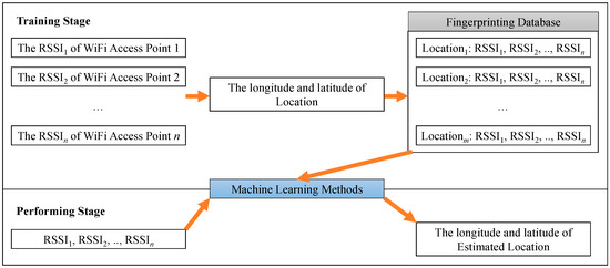
Figure 1. Fingerprinting positioning method. RSSI—received signal strength indication.

For training the mobile positioning models, some studies used k-nearest neighbors, Bayesian theory, support vector machine, neural networks, convolutional neural networks, or recurrent neural networks to estimate locations in accordance with RSSIs. For instance, a probabilistic positioning algorithm was proposed to store the probability distribution of RSSIs during a certain time in the fingerprinting database, and the probable locations of mobile stations were calculated by a Bayesian theory system [10]. However, the relationships among inputs were assumed as independent parameters, so big errors of estimated locations may be obtained if the inputs were not independent parameters. Some mobile positioning methods based on k-nearest neighbor algorithms can obtain higher accuracies of estimated locations, but these methods required more computation time in the performing stage. Some neural networks have been proposed to analyze the interrelated influences of inputs for the improvement of location estimation [8,11,12,13], and convolutional neural networks were applied to extract the features of spatio metrics in accordance with convolutional layers [14,18,19,20,21]. Although the spatio metrics may be analyzed by neural networks and convolutional neural networks, these methods cannot provide the solutions of temporal data analyses. Therefore, this study applies recurrent neural networks to analyze the temporal data for improving the accuracies of estimation locations.

3. Mobile Positioning System and Method

The architecture of the proposed mobile positioning system is presented in Section 3.1, and the concepts of the proposed mobile positioning method are illustrated in Section 3.2.

3.1. Mobile Positioning System

The proposed mobile positioning system includes (1) mobile stations, (2) a mobile positioning server, (3) a database server, and (4) a model server (shown in Figure 2). Each component in the proposed system is presented in the following subsections.

Figure 2. The proposed mobile positioning system.

3.1.1. Mobile Stations

In the training stage, mobile stations can detect and receive the RSSIs of neighbor base stations and Wi-Fi APs from heterogeneous networks. GPS modules can be equipped in the mobile stations and estimate the locations of mobile stations (i.e., coordinates). Then, the mobile stations can send the vectors of GPS coordinates (i.e., longitudes and latitudes) and RSSIs to the mobile positioning server for the collection of network signals. In the performing stage, mobile stations can send the detected RSSIs of neighbor base stations and Wi-Fi APs to the mobile positioning server for location estimation.

3.1.2. Mobile Positioning Server

In the training stage, the mobile positioning server can receive GPS coordinates and network signals (i.e., the RSSIs of base stations and Wi-Fi APs) from mobile stations. These GPS coordinates and network signals can be sent to the database server for storing. The mobile positioning server can execute the proposed mobile positioning method to train RNN models. The network signals can be used as the input layer of the RNN models, and the GPS coordinates can be used as the output layer of the RNN models. Once the RNN models have been trained, these models can be sent to the model server for saving. In the performing stage, the mobile positioning server can load the trained RNN models from the model server. When the mobile positioning server receives network signals from mobile stations, these network signals can be adopted in the trained RNN models for estimating the locations of mobile stations.

3.1.3. Database Server

The database server can store the vectors of coordinates (i.e., longitudes and latitudes) and RSSIs from mobile stations via the mobile positioning server. These vectors can be queried and used to train RNN models.

3.1.4. Model Server

The model server can save the trained RNN models from the mobile positioning server in training stage, and the saved RNN models can be loaded for location estimation by the mobile positioning server.

3.2. Mobile Positioning Method

The proposed mobile positioning method includes (1) collection and normalization, (2) the execution of mobile positioning method based on recurrent neural networks, and (3) de-normalization and estimation. Each step in the proposed method is presented in the following subsections.

3.2.1. Collection and Normalization

For the collection of network signals and GPS coordinates, the RSSIs of base stations from cellular networks (i.e., $R_{c,i}$ in Equation (1)), the RSSIs of Wi-Fi APs from Wi-Fi networks (i.e., $R_{w,i}$ in Equation (2)), and the GPS coordinates (i.e., $l_i$ in Equation (3)) can be detected and collected by the mobile station at time $t_i$ (shown in Figure 3). The RSSI of the j-th base station from a cellular network at time $t_i$ is defined as $r_{c,j,i}$, and the RSSI of the k-th Wi-Fi AP from a Wi-Fi network at time $t_i$ is defined as $r_{w,k,i}$. The RSSI dataset of heterogeneous networks (i.e., cellular networks and Wi-Fi networks) at time $t_i$ is defined as $R_i$ (shown in Equation (4)). Furthermore, the location $l_i$ (i.e., a GPS coordinate) includes a longitude $l_{x,i}$ and a latitude $l_{y,i}$. There are m locations, n₁ different base stations, and n₂ different Wi-Fi APs detected in the experiments. If the RSSIs of base stations or Wi-Fi APs cannot be detected, the values of these RSSIs can be encoded as null. For instance, the mobile station cannot detect the RSSI of Wi-Fi AP2 at time $t_i$ in Figure 3, so the value of $r_{w,2,i}$ is encoded as null.

$$R_{c,i}=\left\{r_{c,1,i},r_{c,2,i},\dots ,r_{c,n_1,i}\right\}$$

(1)

$$R_{w,i}=\left\{r_{w,1,i},r_{w,2,i},\dots ,r_{w,n_2,i}\right\}$$

(2)

$$l_i=\left\{l_{x,i},l_{y,i}\right\}$$

(3)

$$\begin{array}{ll}{R}_i& =\left\{R_{c,i},R_{w,i}\right\}\\ & =\left\{r_{c,1,i},r_{c,2,i},\dots ,r_{c,n_1,i},r_{w,1,i},r_{w,2,i},\dots ,r_{w,n_2,i}\right\}\end{array}$$

(4)

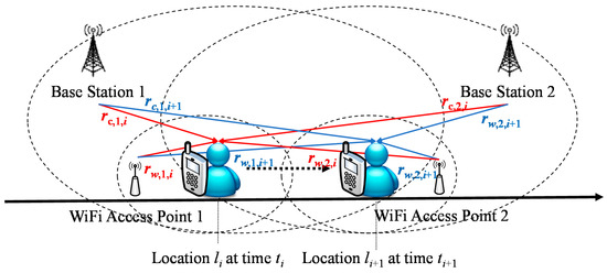
Figure 3. The scenario of network signal and global positioning system (GPS) coordinate collection.

For the normalization of network signals and GPS coordinates, the minimum values and maximum values of RSSIs and coordinates are considered and adopted in Equations (5)–(8). The normalized RSSI of the j-th base station from a cellular network at time $t_i$ is defined as $c_{j,i}$, in accordance with the minimum value and maximum value of the RSSIs (i.e., $r_c^{(-)}$ and $r_c^{(+)}$ in Equation (5)) from cellular networks; the normalized RSSI of the k-th Wi-Fi APs from a cellular network at time $t_i$ is defined as $w_{k,i}$, in accordance with the minimum value and maximum value of the RSSIs (i.e., $r_w^{(-)}$ and $r_w^{(+)}$ in Equation (6)) from Wi-Fi networks. Furthermore, the normalized longitude at time $t_i$ is defined as $x_i$ in accordance with the minimum value and maximum value of longitudes (i.e., $l_x^{(-)}$ and $l_x^{(+)}$ in Equation (7)) from GPS coordinates, and the normalized latitude at time $t_i$ is defined as $y_i$ in accordance with the minimum value and maximum value of latitudes (i.e., $l_y^{(-)}$ and $l_y^{(+)}$ in Equation (8)) from GPS coordinates.

$$c_{j,i}=\{\begin{array}{l}\frac{r_{c,j,i}-r_c^{(-)}}{r_c^{(+)}-r_c^{(-)}},\mathrm{if} r_{c,j,i}\ne null\\ 0,\mathrm{otherwise}\end{array}, \mathrm{where} r_c^{(+)}=\underset{1\le p\le n_1,1\le q\le m}{\max }{r}_{c,p,q}, r_c^{(-)}=\underset{1\le p\le n_1,1\le q\le m}{\min }{r}_{c,p,q}$$

(5)

$$w_{k,i}=\{\begin{array}{l}\frac{r_{w,k,i}-r_w^{(-)}}{r_w^{(+)}-r_w^{(-)}},\mathrm{if} r_{w,k,i}\ne null\\ 0,\mathrm{otherwise}\end{array}, \mathrm{where} r_w^{(+)}=\underset{1\le p\le n_2,1\le q\le m}{\max }{r}_{w,p,q}, r_w^{(-)}=\underset{1\le p\le n_2,1\le q\le m}{\min }{r}_{w,p,q}$$

(6)

$$x_i=\{\begin{array}{l}\frac{l_{x,i}-l_x^{(-)}}{l_x^{(+)}-l_x^{(-)}},\mathrm{if} l_{x,i}\ne null\\ 0,\mathrm{otherwise}\end{array}, \mathrm{where} l_x^{(+)}=\underset{1\le q\le m}{\max }{l}_{x,q}, l_x^{(-)}=\underset{1\le q\le m}{\min }{l}_{x,q}$$

(7)

$$y_i=\{\begin{array}{l}\frac{l_{y,i}-l_y^{(-)}}{l_y^{(+)}-l_y^{(-)}},\mathrm{if} l_{y,i}\ne null\\ 0,\mathrm{otherwise}\end{array}, \mathrm{where} l_y^{(+)}=\underset{1\le q\le m}{\max }{l}_{y,q}, l_y^{(-)}=\underset{1\le q\le m}{\min }{l}_{y,q}$$

(8)

3.2.2. Mobile Positioning Method Based on Recurrent Neural Network

The proposed mobile positioning method adopts recurrent neural network algorithms to estimate the locations of mobile stations. The recurrent neural networks can be applied to extract the features of time series data, so this study considers and analyzes the normalized RSSIs with multiple consecutive timestamps. Section “Recurrent Neural Networks with One Timestamp” presents recurrent neural networks with one timestamp, and Section “Two Timestamps for Recurrent Neural Network” describes recurrent neural networks with multiple consecutive timestamps.

Recurrent Neural Networks with One Timestamp

This subsection shows the designs and optimization of recurrent neural networks with one timestamp. A case study of a recurrent neural network with one timestamp is illustrated in Figure 4. The recurrent neural network is constructed with an input layer, a recurrent hidden layer, and an output layer. The input layer includes the normalized RSSIs of n₁ base stations (i.e., $\left\{c_{1,i},c_{2,i},\dots ,c_{n_1,i}\right\}$) and n₂ Wi-Fi APs (i.e., $\left\{w_{1,i},w_{2,i},\dots ,w_{n_2,i}\right\}$), and the output layer includes the estimated normalized longitude and latitude (i.e., ${\tilde{x}}_i$ and ${\tilde{y}}_i$). The recurrent hidden layer includes a neuron, and the initial value of the neuron in the recurrent hidden layer is defined as h₀. The value of the neuron in the recurrent hidden layer can be updated as h₁ after calculating the RSSIs in the first timestamp. The weights of c_j,i, w_k,i, and h₀ are ${\alpha }_j$, ${\beta }_k$, and v, respectively; the weights of h₁ for the outputs ${\tilde{x}}_i$ and ${\tilde{y}}_i$ are ${\gamma }_1$ and ${\gamma }_2$, respectively. The biases of neurons in the hidden layer and the output layer are defined as b_1,1, b_2,1, and b_3,1. The sigmoid function is elected as the activation function of each neuron, so the values of h₀, h₁, ${\tilde{x}}_i$, and ${\tilde{y}}_i$ can be calculated by Equations (9)–(12), respectively. Furthermore, the loss function is defined as Equation (13) in accordance with squared errors.

$$h_0=0$$

(9)

$$h_1=s\left({\displaystyle \sum _{j=1}^{n_1}{\alpha }_j\times c_{j,i}}+{\displaystyle \sum _{k=1}^{n_2}{\beta }_k\times w_{k,i}}+v\times h_0+b_{1,1}\right)=s\left(z_{1,1}\right), \mathrm{where} s\left(z\right)=\frac{1}{1+e^{-z}}$$

(10)

$${\tilde{x}}_i=s\left({\gamma }_1\times h_1+b_{2,1}\right)=s\left(z_{2,1}\right), \mathrm{where} s\left(z\right)=\frac{1}{1+e^{-z}}$$

(11)

$${\tilde{y}}_i=s\left({\gamma }_2\times h_1+b_{3,1}\right)=s\left(z_{3,1}\right), \mathrm{where} s\left(z\right)=\frac{1}{1+e^{-z}}$$

(12)

$$E=\frac{1}{2}{\left({\tilde{x}}_i-x_i\right)}^2+\frac{1}{2}{\left({\tilde{y}}_i-y_i\right)}^2=\frac{1}{2}{\sigma }_1{}^2+\frac{1}{2}{\sigma }_2{}^2$$

(13)

Figure 4. A recurrent neural network with one timestamp.

For the optimization of recurrent neural network, the learning rate $\eta$ and a gradient descent method is applied to update each weight and bias. The updates of ${\gamma }_1$, ${\gamma }_2$, $b_{2,1}$, $b_{3,1}$, ${\alpha }_j$, ${\beta }_k$, $v$, and $b_{1,1}$ are proven and calculated by Equations (14)–(21), respectively.

$$\begin{array}{l}\begin{array}{l}{\gamma }_1={\gamma }_1-\eta \times \frac{\partial E}{\partial {\gamma }_1}, \mathrm{where}\end{array}\\ \begin{array}{ll}\frac{\partial E}{\partial {\gamma }_1}& =\frac{\partial E}{\partial {\sigma }_1}\frac{\partial {\sigma }_1}{\partial {\tilde{x}}_i}\frac{\partial {\tilde{x}}_i}{\partial z_{2,1}}\frac{\partial z_{2,1}}{\partial {\gamma }_1}+\frac{\partial E}{\partial {\sigma }_2}\frac{\partial {\sigma }_2}{\partial {\tilde{y}}_i}\frac{\partial {\tilde{y}}_i}{\partial z_{3,1}}\frac{\partial z_{3,1}}{\partial {\gamma }_1}\\ & ={\sigma }_1\times {\tilde{x}}_i\times \left[1-{\tilde{x}}_i\right]\times h_1\end{array}\end{array}$$

(14)

$$\begin{array}{l}\begin{array}{l}{\gamma }_2={\gamma }_2-\eta \times \frac{\partial E}{\partial {\gamma }_2}, \mathrm{where}\end{array}\\ \begin{array}{ll}\frac{\partial E}{\partial {\gamma }_2}& =\frac{\partial E}{\partial {\sigma }_1}\frac{\partial {\sigma }_{1,}}{\partial {\tilde{x}}_i}\frac{\partial {\tilde{x}}_i}{\partial z_{2,1}}\frac{\partial z_{2,1}}{\partial {\gamma }_2}+\frac{\partial E}{\partial {\sigma }_2}\frac{\partial {\sigma }_2}{\partial {\tilde{y}}_i}\frac{\partial {\tilde{y}}_i}{\partial z_{3,1}}\frac{\partial z_{3,1}}{\partial {\gamma }_2}\\ & ={\sigma }_2\times {\tilde{y}}_i\times \left[1-{\tilde{y}}_i\right]\times h_1\end{array}\end{array}$$

(15)

$$\begin{array}{l}\begin{array}{l}{b}_{2,1}=b_{2,1}-\eta \times \frac{\partial E}{\partial b_{2,1}}, \mathrm{where}\end{array}\\ \begin{array}{ll}\frac{\partial E}{\partial b_{2,1}}& =\frac{\partial E}{\partial {\sigma }_1}\frac{\partial {\sigma }_1}{\partial {\tilde{x}}_i}\frac{\partial {\tilde{x}}_i}{\partial z_{2,1}}\frac{\partial z_{2,1}}{\partial b_{2,1}}+\frac{\partial E}{\partial {\sigma }_2}\frac{\partial {\sigma }_2}{\partial {\tilde{y}}_i}\frac{\partial {\tilde{y}}_i}{\partial z_{3,1}}\frac{\partial z_{3,1}}{\partial b_{2,1}}\\ & ={\sigma }_1\times {\tilde{x}}_i\times \left[1-{\tilde{x}}_i\right]\end{array}\end{array}$$

(16)

$$\begin{array}{l}\begin{array}{l}{b}_{3,1}=b_{3,1}-\eta \times \frac{\partial E}{\partial b_{3,1}}, \mathrm{where}\end{array}\\ \begin{array}{ll}\frac{\partial E}{\partial b_{3,1}}& =\frac{\partial E}{\partial {\sigma }_1}\frac{\partial {\sigma }_1}{\partial {\tilde{x}}_i}\frac{\partial {\tilde{x}}_i}{\partial z_{2,1}}\frac{\partial z_{2,1}}{\partial b_{3,1}}+\frac{\partial E}{\partial {\sigma }_2}\frac{\partial {\sigma }_2}{\partial {\tilde{y}}_i}\frac{\partial {\tilde{y}}_i}{\partial z_{3,1}}\frac{\partial z_{3,1}}{\partial b_{3,1}}\\ & ={\sigma }_2\times {\tilde{y}}_i\times \left[1-{\tilde{y}}_i\right]\end{array}\end{array}$$

(17)

$$\begin{array}{l}\begin{array}{l}{\alpha }_j={\alpha }_j-\eta \times \frac{\partial E}{\partial {\alpha }_j}, \mathrm{where}\end{array}\\ \begin{array}{ll}\frac{\partial E}{\partial {\alpha }_j}& =\frac{\partial E}{\partial {\sigma }_1}\frac{\partial {\sigma }_1}{\partial {\tilde{x}}_i}\frac{\partial {\tilde{x}}_i}{\partial z_{2,1}}\frac{\partial z_{2,1}}{\partial h_1}\frac{\partial h_1}{\partial z_{1,1}}\frac{\partial z_{1,1}}{\partial {\alpha }_1}+\frac{\partial E}{\partial {\sigma }_2}\frac{\partial {\sigma }_2}{\partial {\tilde{y}}_i}\frac{\partial {\tilde{y}}_i}{\partial z_{3,1}}\frac{\partial z_{3,1}}{\partial h_1}\frac{\partial h_1}{\partial z_{1,1}}\frac{\partial z_{1,1}}{\partial {\alpha }_j}\\ & =\left(\frac{\partial E}{\partial {\sigma }_1}\frac{\partial {\sigma }_1}{\partial {\tilde{x}}_i}\frac{\partial {\tilde{x}}_i}{\partial z_{2,1}}\frac{\partial z_{2,1}}{\partial h_1}+\frac{\partial E}{\partial {\sigma }_2}\frac{\partial {\sigma }_2}{\partial {\tilde{y}}_i}\frac{\partial {\tilde{y}}_i}{\partial z_{3,1}}\frac{\partial z_{3,1}}{\partial h_1}\right)\frac{\partial h_1}{\partial z_{1,1}}\frac{\partial z_{1,1}}{\partial {\alpha }_j}\\ & =\left\{{\sigma }_1\times {\tilde{x}}_i\times \left[1-{\tilde{x}}_i\right]\times {\gamma }_1+{\sigma }_2\times {\tilde{y}}_i\times \left[1-{\tilde{y}}_i\right]\times {\gamma }_2\right\}\times h_1\times \left[1-h_1\right]\times c_{j,i}\end{array}\end{array}$$

(18)

$$\begin{array}{l}\begin{array}{l}{\beta }_k={\beta }_k-\eta \times \frac{\partial E}{\partial {\beta }_k}, \mathrm{where}\end{array}\\ \begin{array}{ll}\frac{\partial E}{\partial {\beta }_k}& =\frac{\partial E}{\partial {\sigma }_1}\frac{\partial {\sigma }_1}{\partial {\tilde{x}}_i}\frac{\partial {\tilde{x}}_i}{\partial z_{2,1}}\frac{\partial z_{2,1}}{\partial h_1}\frac{\partial h_1}{\partial z_{1,1}}\frac{\partial z_{1,1}}{\partial {\alpha }_2}+\frac{\partial E}{\partial {\sigma }_2}\frac{\partial {\sigma }_2}{\partial {\tilde{y}}_i}\frac{\partial {\tilde{y}}_i}{\partial z_{3,1}}\frac{\partial z_{3,1}}{\partial h_1}\frac{\partial h_1}{\partial z_{1,1}}\frac{\partial z_{1,1}}{\partial {\beta }_k}\\ & =\left(\frac{\partial E}{\partial {\sigma }_1}\frac{\partial {\sigma }_1}{\partial {\tilde{x}}_i}\frac{\partial {\tilde{x}}_i}{\partial z_{2,1}}\frac{\partial z_{2,1}}{\partial h_1}+\frac{\partial E}{\partial {\sigma }_2}\frac{\partial {\sigma }_2}{\partial {\tilde{y}}_i}\frac{\partial {\tilde{y}}_i}{\partial z_{3,1}}\frac{\partial z_{3,1}}{\partial h_1}\right)\frac{\partial h_1}{\partial z_{1,1}}\frac{\partial z_{1,1}}{\partial {\beta }_k}\\ & =\left\{{\sigma }_1\times {\tilde{x}}_i\times \left[1-{\tilde{x}}_i\right]\times {\gamma }_1+{\sigma }_2\times {\tilde{y}}_i\times \left[1-{\tilde{y}}_i\right]\times {\gamma }_2\right\}\times h_1\times \left[1-h_1\right]\times w_{k,i}\end{array}\end{array}$$

(19)

$$\begin{array}{l}\begin{array}{l}v=v-\eta \times \frac{\partial E}{\partial v}, \mathrm{where}\end{array}\\ \begin{array}{ll}\frac{\partial E}{\partial v}& =\frac{\partial E}{\partial {\sigma }_1}\frac{\partial {\sigma }_1}{\partial {\tilde{x}}_i}\frac{\partial {\tilde{x}}_i}{\partial z_{2,1}}\frac{\partial z_{2,1}}{\partial h_1}\frac{\partial h_1}{\partial z_{1,1}}\frac{\partial z_{1,1}}{\partial v}+\frac{\partial E}{\partial {\sigma }_2}\frac{\partial {\sigma }_2}{\partial {\tilde{y}}_i}\frac{\partial {\tilde{y}}_i}{\partial z_{3,1}}\frac{\partial z_{3,1}}{\partial h_1}\frac{\partial h_1}{\partial z_{1,1}}\frac{\partial z_{1,1}}{\partial v}\\ & =\left(\frac{\partial E}{\partial {\sigma }_1}\frac{\partial {\sigma }_1}{\partial {\tilde{x}}_i}\frac{\partial {\tilde{x}}_i}{\partial z_{2,1}}\frac{\partial z_{2,1}}{\partial h_1}+\frac{\partial E}{\partial {\sigma }_2}\frac{\partial {\sigma }_2}{\partial {\tilde{y}}_i}\frac{\partial {\tilde{y}}_i}{\partial z_{3,1}}\frac{\partial z_{3,1}}{\partial h_1}\right)\frac{\partial h_1}{\partial z_{1,1}}\frac{\partial z_{1,1}}{\partial v}\\ & =\left\{{\sigma }_1\times {\tilde{x}}_i\times \left[1-{\tilde{x}}_i\right]\times {\gamma }_1+{\sigma }_2\times {\tilde{y}}_i\times \left[1-{\tilde{y}}_i\right]\times {\gamma }_2\right\}\times h_1\times \left[1-h_1\right]\times h_0\end{array}\end{array}$$

(20)

$$\begin{array}{l}\begin{array}{l}{b}_{1,1}=b_{1,1}-\eta \times \frac{\partial E}{\partial b_{1,1}}, \mathrm{where}\end{array}\\ \begin{array}{ll}\frac{\partial E}{\partial b_{1,1}}& =\frac{\partial E}{\partial {\sigma }_1}\frac{\partial {\sigma }_1}{\partial {\tilde{x}}_i}\frac{\partial {\tilde{x}}_i}{\partial z_{2,1}}\frac{\partial z_{2,1}}{\partial h_1}\frac{\partial h_1}{\partial z_{1,1}}\frac{\partial z_{1,1}}{\partial b_{1,1}}+\frac{\partial E}{\partial {\sigma }_2}\frac{\partial {\sigma }_2}{\partial {\tilde{y}}_i}\frac{\partial {\tilde{y}}_i}{\partial z_{3,1}}\frac{\partial z_{3,1}}{\partial h_1}\frac{\partial h_1}{\partial z_{1,1}}\frac{\partial z_{1,1}}{\partial b_{1,1}}\\ & =\left(\frac{\partial E}{\partial {\sigma }_1}\frac{\partial {\sigma }_1}{\partial {\tilde{x}}_i}\frac{\partial {\tilde{x}}_i}{\partial z_{2,1}}\frac{\partial z_{2,1}}{\partial h_1}+\frac{\partial E}{\partial {\sigma }_2}\frac{\partial {\sigma }_2}{\partial {\tilde{y}}_i}\frac{\partial {\tilde{y}}_i}{\partial z_{3,1}}\frac{\partial z_{3,1}}{\partial h_1}\right)\frac{\partial h_1}{\partial z_{1,1}}\frac{\partial z_{1,1}}{\partial b_{1,1}}\\ & =\left\{{\sigma }_1\times {\tilde{x}}_i\times \left[1-{\tilde{x}}_i\right]\times {\gamma }_1+{\sigma }_2\times {\tilde{y}}_i\times \left[1-{\tilde{y}}_i\right]\times {\gamma }_2\right\}\times h_1\times \left[1-h_1\right]\end{array}\end{array}$$

(21)

Furthermore, the number of neurons in the recurrent hidden layer can be extended for the extraction of time series data. The weight between each of the two neurons can be updated by the gradient descent method.

Two Timestamps for Recurrent Neural Network

This subsection illustrates the designs and optimization of recurrent neural networks with two consecutive timestamps. A case study of a recurrent neural network with two consecutive timestamps is showed in Figure 5. In the case, the recurrent neural network is constructed with an input layer, a recurrent hidden layer, and an output layer. The input layer includes (n₁ + n₂) normalized RSSIs (i.e., $\left\{c_{1,i},c_{2,i},\dots ,c_{n_1,i}\right\}$ and $\left\{w_{1,i},w_{2,i},\dots ,w_{n_2,i}\right\}$) in the first timestamp and (n₁ + n₂) normalized RSSIs (i.e., $\left\{c_{1,i+1},c_{2,i+1},\dots ,c_{n_1,i+1}\right\}$ and $\left\{w_{1,i+1},w_{2,i+1},\dots ,w_{n_2,i+1}\right\}$) in the second timestamp; the output layer includes the estimated normalized longitude and latitude (i.e., ${\tilde{x}}_{i+1}$ and ${\tilde{y}}_{i+1}$) in the second timestamp. The recurrent hidden layer includes a neuron, and the initial value of the neuron in the recurrent hidden layer is defined as h₀ (shown in Equation (9)). The value of the neuron in the recurrent hidden layer can be updated as h₁ in the first timestamp and as h₂ in the second timestamp. The weights of base station j, Wi-Fi AP k in each timestamp are ${\alpha }_j$ and ${\beta }_k$; the weights of h₂ for the outputs ${\tilde{x}}_{i+1}$ and ${\tilde{y}}_{i+1}$ are ${\gamma }_1$ and ${\gamma }_2$, respectively. Furthermore, the weight of the neurons in the recurrent hidden layer in the least timestamp is defined as v. In the case, the biases of neurons in the hidden layer and the output layer are defined as b_1,1, b_2,1, and b_3,1. The sigmoid function is elected as the activation function of each neuron, so the values of h₁, h₂, ${\tilde{x}}_i$, and ${\tilde{y}}_i$ can be calculated by Equations (22)–(25), respectively. Furthermore, the loss function is defined as Equation (26) in accordance with squared errors.

$$h_1=s\left({\displaystyle \sum _{j=1}^{n_1}{\alpha }_j\times c_{j,i}}+{\displaystyle \sum _{k=1}^{n_2}{\beta }_k\times w_{k,i}}+v\times h_0+b_{1,1}\right)=s\left(z_{1,1}\right), \mathrm{where} s\left(z\right)=\frac{1}{1+e^{-z}}$$

(22)

$$h_2=s\left({\displaystyle \sum _{j=1}^{n_1}{\alpha }_j\times c_{j,i+1}}+{\displaystyle \sum _{k=1}^{n_2}{\beta }_k\times w_{k,i+1}}+v\times h_1+b_{1,1}\right)=s\left(z_{1,2}\right), \mathrm{where} s\left(z\right)=\frac{1}{1+e^{-z}}$$

(23)

$${\tilde{x}}_{i+1}=s\left({\gamma }_1\times h_2+b_{2,1}\right)=s\left(z_{2,1}\right), \mathrm{where} s\left(z\right)=\frac{1}{1+e^{-z}}$$

(24)

$${\tilde{y}}_{i+1}=s\left({\gamma }_2\times h_2+b_{3,1}\right)=s\left(z_{3,1}\right), \mathrm{where} s\left(z\right)=\frac{1}{1+e^{-z}}$$

(25)

$$E=\frac{1}{2}{\left({\tilde{x}}_{i+1}-x_{i+1}\right)}^2+\frac{1}{2}{\left({\tilde{y}}_{i+1}-y_{i+1}\right)}^2=\frac{1}{2}{\sigma }_1{}^2+\frac{1}{2}{\sigma }_2{}^2$$

(26)

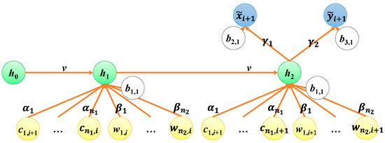
Figure 5. A recurrent neural network with two consecutive timestamps.

For the optimization of recurrent neural network with two consecutive timestamps, the learning rate $\eta$ and a gradient descent method is applied to update each weight and bias. The updates of ${\gamma }_1$, ${\gamma }_2$, $b_{2,1}$, $b_{3,1}$, ${\alpha }_j$, ${\beta }_k$, $v$, and $b_{1,1}$ are proven and calculated by Equations (27)–(34), respectively.

$$\begin{array}{l}\begin{array}{l}{\gamma }_1={\gamma }_1-\eta \times \frac{\partial E}{\partial {\gamma }_1}, \mathrm{where}\end{array}\\ \begin{array}{ll}\frac{\partial E}{\partial {\gamma }_1}& =\frac{\partial E}{\partial {\sigma }_1}\frac{\partial {\sigma }_1}{\partial {\tilde{x}}_{i+1}}\frac{\partial {\tilde{x}}_{i+1}}{\partial z_{2,1}}\frac{\partial z_{2,1}}{\partial {\gamma }_1}+\frac{\partial E}{\partial {\sigma }_2}\frac{\partial {\sigma }_2}{\partial {\tilde{y}}_{i+1}}\frac{\partial {\tilde{y}}_{i+1}}{\partial z_{3,1}}\frac{\partial z_{3,1}}{\partial {\gamma }_1}\\ & ={\sigma }_1\times {\tilde{x}}_{i+1}\times \left[1-{\tilde{x}}_{i+1}\right]\times h_2\end{array}\end{array}$$

(27)

$$\begin{array}{l}\begin{array}{l}{\gamma }_2={\gamma }_2-\eta \times \frac{\partial E}{\partial {\gamma }_2}, \mathrm{where}\end{array}\\ \begin{array}{ll}\frac{\partial E}{\partial {\gamma }_2}& =\frac{\partial E}{\partial {\sigma }_1}\frac{\partial {\sigma }_{1,}}{\partial {\tilde{x}}_{i+1}}\frac{\partial {\tilde{x}}_{i+1}}{\partial z_{2,1}}\frac{\partial z_{2,1}}{\partial {\gamma }_2}+\frac{\partial E}{\partial {\sigma }_2}\frac{\partial {\sigma }_2}{\partial {\tilde{y}}_{i+1}}\frac{\partial {\tilde{y}}_{i+1}}{\partial z_{3,1}}\frac{\partial z_{3,1}}{\partial {\gamma }_2}\\ & ={\sigma }_2\times {\tilde{y}}_{i+1}\times \left[1-{\tilde{y}}_{i+1}\right]\times h_2\end{array}\end{array}$$

(28)

$$\begin{array}{l}\begin{array}{l}{b}_{2,1}=b_{2,1}-\eta \times \frac{\partial E}{\partial b_{2,1}}, \mathrm{where}\end{array}\\ \begin{array}{ll}\frac{\partial E}{\partial b_{2,1}}& =\frac{\partial E}{\partial {\sigma }_1}\frac{\partial {\sigma }_1}{\partial {\tilde{x}}_{i+1}}\frac{\partial {\tilde{x}}_{i+1}}{\partial z_{2,1}}\frac{\partial z_{2,1}}{\partial b_{2,1}}+\frac{\partial E}{\partial {\sigma }_2}\frac{\partial {\sigma }_2}{\partial {\tilde{y}}_{i+1}}\frac{\partial {\tilde{y}}_{i+1}}{\partial z_{3,1}}\frac{\partial z_{3,1}}{\partial b_{2,1}}\\ & ={\sigma }_1\times {\tilde{x}}_{i+1}\times \left[1-{\tilde{x}}_{i+1}\right]\end{array}\end{array}$$

(29)

$$\begin{array}{l}\begin{array}{l}{b}_{3,1}=b_{3,1}-\eta \times \frac{\partial E}{\partial b_{3,1}}, \mathrm{where}\end{array}\\ \begin{array}{ll}\frac{\partial E}{\partial b_{3,1}}& =\frac{\partial E}{\partial {\sigma }_1}\frac{\partial {\sigma }_1}{\partial {\tilde{x}}_{i+1}}\frac{\partial {\tilde{x}}_{i+1}}{\partial z_{2,1}}\frac{\partial z_{2,1}}{\partial b_{3,1}}+\frac{\partial E}{\partial {\sigma }_2}\frac{\partial {\sigma }_2}{\partial {\tilde{y}}_{i+1}}\frac{\partial {\tilde{y}}_{i+1}}{\partial z_{3,1}}\frac{\partial z_{3,1}}{\partial b_{3,1}}\\ & ={\sigma }_2\times {\tilde{y}}_{i+1}\times \left[1-{\tilde{y}}_{i+1}\right]\end{array}\end{array}$$

(30)

$$\begin{array}{l}\begin{array}{l}{\alpha }_j={\alpha }_j-\eta \times \frac{\partial E}{\partial {\alpha }_j}, \mathrm{where}\end{array}\\ \begin{array}{ll}\frac{\partial E}{\partial {\alpha }_j}& =\frac{\partial E}{\partial {\sigma }_1}\frac{\partial {\sigma }_1}{\partial {\tilde{x}}_{i+1}}\frac{\partial {\tilde{x}}_{i+1}}{\partial z_{2,1}}\frac{\partial z_{2,1}}{\partial h_2}\frac{\partial h_2}{\partial z_{1,2}}\frac{\partial z_{1,2}}{\partial {\alpha }_1}+\frac{\partial E}{\partial {\sigma }_2}\frac{\partial {\sigma }_2}{\partial {\tilde{y}}_{i+1}}\frac{\partial {\tilde{y}}_{i+1}}{\partial z_{3,1}}\frac{\partial z_{3,1}}{\partial h_2}\frac{\partial h_2}{\partial z_{1,2}}\frac{\partial z_{1,2}}{\partial {\alpha }_j}\\ & =\left(\frac{\partial E}{\partial {\sigma }_1}\frac{\partial {\sigma }_1}{\partial {\tilde{x}}_{i+1}}\frac{\partial {\tilde{x}}_{i+1}}{\partial z_{2,1}}\frac{\partial z_{2,1}}{\partial h_2}+\frac{\partial E}{\partial {\sigma }_2}\frac{\partial {\sigma }_2}{\partial {\tilde{y}}_{i+1}}\frac{\partial {\tilde{y}}_{i+1}}{\partial z_{3,1}}\frac{\partial z_{3,1}}{\partial h_2}\right)\frac{\partial h_2}{\partial z_{1,2}}\frac{\partial z_{1,2}}{\partial {\alpha }_j}\\ & =\left\{{\sigma }_1\times {\tilde{x}}_{i+1}\times \left[1-{\tilde{x}}_{i+1}\right]\times {\gamma }_1+{\sigma }_2\times {\tilde{y}}_{i+1}\times \left[1-{\tilde{y}}_{i+1}\right]\times {\gamma }_2\right\}\times h_2\times \left[1-h_2\right]\times \left(c_{j,i+1}+v\frac{\partial h_1}{\partial z_{1,1}}\frac{\partial z_{1,1}}{\partial {\alpha }_j}\right)\\ & =\left\{{\sigma }_1\times {\tilde{x}}_{i+1}\times \left[1-{\tilde{x}}_{i+1}\right]\times {\gamma }_1+{\sigma }_2\times {\tilde{y}}_{i+1}\times \left[1-{\tilde{y}}_{i+1}\right]\times {\gamma }_2\right\}\times h_2\times \left[1-h_2\right]\times \left(c_{j,i+1}+v\times h_1\times \left[1-h_1\right]\times c_{j,i}\right)\end{array}\end{array}$$

(31)

$$\begin{array}{l}\begin{array}{l}{\beta }_k={\beta }_k-\eta \times \frac{\partial E}{\partial {\beta }_k}, \mathrm{where}\end{array}\\ \begin{array}{ll}\frac{\partial E}{\partial {\beta }_k}& =\frac{\partial E}{\partial {\sigma }_1}\frac{\partial {\sigma }_1}{\partial {\tilde{x}}_{i+1}}\frac{\partial {\tilde{x}}_{i+1}}{\partial z_{2,1}}\frac{\partial z_{2,1}}{\partial h_2}\frac{\partial h_2}{\partial z_{1,2}}\frac{\partial z_{1,2}}{\partial {\alpha }_2}+\frac{\partial E}{\partial {\sigma }_2}\frac{\partial {\sigma }_2}{\partial {\tilde{y}}_{i+1}}\frac{\partial {\tilde{y}}_{i+1}}{\partial z_{3,1}}\frac{\partial z_{3,1}}{\partial h_2}\frac{\partial h_2}{\partial z_{1,2}}\frac{\partial z_{1,2}}{\partial {\beta }_k}\\ & =\left(\frac{\partial E}{\partial {\sigma }_1}\frac{\partial {\sigma }_1}{\partial {\tilde{x}}_{i+1}}\frac{\partial {\tilde{x}}_{i+1}}{\partial z_{2,1}}\frac{\partial z_{2,1}}{\partial h_2}+\frac{\partial E}{\partial {\sigma }_2}\frac{\partial {\sigma }_2}{\partial {\tilde{y}}_{i+1}}\frac{\partial {\tilde{y}}_{i+1}}{\partial z_{3,1}}\frac{\partial z_{3,1}}{\partial h_2}\right)\frac{\partial h_2}{\partial z_{1,2}}\frac{\partial z_{1,2}}{\partial {\beta }_k}\\ & =\left\{{\sigma }_1\times {\tilde{x}}_{i+1}\times \left[1-{\tilde{x}}_{i+1}\right]\times {\gamma }_1+{\sigma }_2\times {\tilde{y}}_{i+1}\times \left[1-{\tilde{y}}_{i+1}\right]\times {\gamma }_2\right\}\times h_2\times \left[1-h_2\right]\times \left(w_{k,i+1}+v\frac{\partial h_1}{\partial z_{1,1}}\frac{\partial z_{1,1}}{\partial {\beta }_k}\right)\\ & =\left\{{\sigma }_1\times {\tilde{x}}_{i+1}\times \left[1-{\tilde{x}}_{i+1}\right]\times {\gamma }_1+{\sigma }_2\times {\tilde{y}}_{i+1}\times \left[1-{\tilde{y}}_{i+1}\right]\times {\gamma }_2\right\}\times h_2\times \left[1-h_2\right]\times \left(w_{k,i+1}+v\times h_1\times \left[1-h_1\right]\times w_{k,i}\right)\end{array}\end{array}$$

(32)

$$\begin{array}{l}\begin{array}{l}v=v-\eta \times \frac{\partial E}{\partial v}, \mathrm{where}\end{array}\\ \begin{array}{ll}\frac{\partial E}{\partial v}& =\frac{\partial E}{\partial {\sigma }_1}\frac{\partial {\sigma }_1}{\partial {\tilde{x}}_{i+1}}\frac{\partial {\tilde{x}}_{i+1}}{\partial z_{2,1}}\frac{\partial z_{2,1}}{\partial h_2}\frac{\partial h_2}{\partial z_{1,2}}\frac{\partial z_{1,2}}{\partial v}+\frac{\partial E}{\partial {\sigma }_2}\frac{\partial {\sigma }_2}{\partial {\tilde{y}}_{i+1}}\frac{\partial {\tilde{y}}_{i+1}}{\partial z_{3,1}}\frac{\partial z_{3,1}}{\partial h_2}\frac{\partial h_2}{\partial z_{1,2}}\frac{\partial z_{1,2}}{\partial v}\\ & =\left(\frac{\partial E}{\partial {\sigma }_1}\frac{\partial {\sigma }_1}{\partial {\tilde{x}}_{i+1}}\frac{\partial {\tilde{x}}_{i+1}}{\partial z_{2,1}}\frac{\partial z_{2,1}}{\partial h_2}+\frac{\partial E}{\partial {\sigma }_2}\frac{\partial {\sigma }_2}{\partial {\tilde{y}}_{i+1}}\frac{\partial {\tilde{y}}_{i+1}}{\partial z_{3,1}}\frac{\partial z_{3,1}}{\partial h_2}\right)\frac{\partial h_2}{\partial z_{1,2}}\frac{\partial z_{1,2}}{\partial v}\\ & =\left\{{\sigma }_1\times {\tilde{x}}_{i+1}\times \left[1-{\tilde{x}}_{i+1}\right]\times {\gamma }_1+{\sigma }_2\times {\tilde{y}}_{i+1}\times \left[1-{\tilde{y}}_{i+1}\right]\times {\gamma }_2\right\}\times h_2\times \left[1-h_2\right]\times \left(\frac{\partial v}{\partial v}{h}_1+v\times \frac{\partial h_1}{\partial z_{1,1}}\frac{\partial z_{1,1}}{\partial v}\right)\\ & =\left\{{\sigma }_1\times {\tilde{x}}_{i+1}\times \left[1-{\tilde{x}}_{i+1}\right]\times {\gamma }_1+{\sigma }_2\times {\tilde{y}}_{i+1}\times \left[1-{\tilde{y}}_{i+1}\right]\times {\gamma }_2\right\}\times h_2\times \left[1-h_2\right]\times \left(h_1+v\times h_1\times \left[1-h_1\right]\times h_0\right)\end{array}\end{array}$$

(33)

$$\begin{array}{l}\begin{array}{l}{b}_{1,1}=b_{1,1}-\eta \times \frac{\partial E}{\partial b_{1,1}}, \mathrm{where}\end{array}\\ \begin{array}{ll}\frac{\partial E}{\partial b_{1,1}}& =\frac{\partial E}{\partial {\sigma }_1}\frac{\partial {\sigma }_1}{\partial {\tilde{x}}_{i+1}}\frac{\partial {\tilde{x}}_{i+1}}{\partial z_{2,1}}\frac{\partial z_{2,1}}{\partial h_2}\frac{\partial h_2}{\partial z_{1,2}}\frac{\partial z_{1,2}}{\partial b_{1,1}}+\frac{\partial E}{\partial {\sigma }_2}\frac{\partial {\sigma }_2}{\partial {\tilde{y}}_{i+1}}\frac{\partial {\tilde{y}}_{i+1}}{\partial z_{3,1}}\frac{\partial z_{3,1}}{\partial h_2}\frac{\partial h_2}{\partial z_{1,2}}\frac{\partial z_{1,2}}{\partial b_{1,1}}\\ & =\left(\frac{\partial E}{\partial {\sigma }_1}\frac{\partial {\sigma }_1}{\partial {\tilde{x}}_{i+1}}\frac{\partial {\tilde{x}}_{i+1}}{\partial z_{2,1}}\frac{\partial z_{2,1}}{\partial h_2}+\frac{\partial E}{\partial {\sigma }_2}\frac{\partial {\sigma }_2}{\partial {\tilde{y}}_{i+1}}\frac{\partial {\tilde{y}}_{i+1}}{\partial z_{3,1}}\frac{\partial z_{3,1}}{\partial h_2}\right)\frac{\partial h_2}{\partial z_{1,2}}\frac{\partial z_{1,2}}{\partial b_{1,1}}\\ & =\left\{{\sigma }_1\times {\tilde{x}}_{i+1}\times \left[1-{\tilde{x}}_{i+1}\right]\times {\gamma }_1+{\sigma }_2\times {\tilde{y}}_{i+1}\times \left[1-{\tilde{y}}_{i+1}\right]\times {\gamma }_2\right\}\times h_2\times \left[1-h_2\right]\times \left(1+v\frac{\partial h_1}{\partial z_{1,1}}\frac{\partial z_{1,1}}{\partial b_{1,1}}\right)\\ & =\left\{{\sigma }_1\times {\tilde{x}}_{i+1}\times \left[1-{\tilde{x}}_{i+1}\right]\times {\gamma }_1+{\sigma }_2\times {\tilde{y}}_{i+1}\times \left[1-{\tilde{y}}_{i+1}\right]\times {\gamma }_2\right\}\times h_2\times \left[1-h_2\right]\times \left(1+v\times h_1\times \left[1-h_1\right]\right)\end{array}\end{array}$$

(34)

Furthermore, the recurrent neural network can analyze with more consecutive timestamps, and the number of neurons in the recurrent hidden layer of the recurrent neural network can be extended for the extraction of time series data. The weight between each of the two neurons can be updated by the gradient descent method.

3.2.3. De-Normalization and Estimation

For de-normalization and estimation, the estimated normalized longitude and latitude (i.e., ${\tilde{x}}_i$ and ${\tilde{y}}_i$) can be adopted in Equations (35) and (36) to retrieve the estimated longitude and latitude (i.e., ${\tilde{l}}_{x,i}$ and ${\tilde{l}}_{y,i}$), respectively.

$${\tilde{l}}_{x,i}={\tilde{x}}_i\times \left(l_x^{(+)}-l_x^{(-)}\right)+l_x^{(-)}$$

(35)

$${\tilde{l}}_{y,i}={\tilde{y}}_i\times \left(l_y^{(+)}-l_y^{(-)}\right)+l_y^{(-)}$$

(36)

4. Practical Experimental Results and Discussion

This section presents and discusses the practical experimental results. Practical experimental environments are illustrated in Section 4.1, and practical experimental results are shown in Section 4.2. Section 4.3 discusses the results of different recurrent neural networks.

4.1. Practical Experimental Environments

In the practical experimental environments, an Android application was implemented and installed into mobile stations (e.g., Redmi 5 running Android platform 7.1.2). The Android application was performed to collect the coordinates of the GPS module and the RSSIs from cellular networks and Wi-Fi networks every second. The mobile stations were carried out on a 5.6 km long road segment in Fuzhou University in China (shown in Figure 6). The segment was traversed eight times by the same mobile station to collect GPS coordinates and network signals (i.e., the RSSIs of base stations and Wi-Fi APs). There are 4525 records (i.e., m = 4525), 59 different base stations (i.e., n₁ = 59) in long term evolution (LTE) networks, and 582 different Wi-Fi APs (i.e., n₂ = 582) detected in the experiments. The availability of position method based on cellular networks was 100%, but the availability of position method based on Wi-Fi networks was about 96%. Some road segments in experimental environments were not covered by Wi-Fi networks. Therefore, the proposed method based Wi-Fi network signals for outdoor, but in range of a nearby Wi-Fi networks. This study selected 2263 records including GPS coordinates and RSSIs as training data, and other 2262 records were selected as testing data. The mean and median of distances between each of the two measurement locations along the test route were 2.8 and 2.6 m, respectively.

Figure 6. Practical experimental environments.

4.2. Practical Experimental Results

For the evaluation of the proposed mobile positioning method, nine experimental cases with different timestamp numbers (i.e., one timestamp, two timestamps, and three timestamps) and with different mobile networks (i.e., only cellular networks, only Wi-Fi networks, and cellular and Wi-Fi networks) were designed and performed. There were 30 neurons in the recurrent hidden layer of the recurrent neural network for each experimental case. The practical experimental results are shown in Table 1, as well as in Figure 7, Figure 8, Figure 9 and Figure 10. Table 1 and Figure 7 illustrated that the more precise location can be estimated by the proposed method with heterogeneous networks (i.e., long term evolution networks and Wi-Fi networks). The higher location errors may be obtained by the recurrent neural networks with one timestamp (i.e., traditional neural networks), which cannot extract the feature of time series data (shown in Table 1 and Figure 8). The lower location errors can be obtained by the recurrent neural networks with multiple consecutive timestamps (e.g., two timestamps and three timestamps); from the experimental results, it can be observed that the average error of location estimation was 9.19 m by the proposed mobile positioning method with two timestamps.

Table 1. The average errors of estimated locations by the proposed mobile positioning method (unit: meters).

Number of Timestamps	Only Cellular Networks	Only Wi-Fi Networks	Cellular and Wi-Fi Networks
1 timestamp	39.88	18.88	16.21
2 timestamps	36.51	18.69	9.19
3 timestamps	34.57	17.83	9.26

Figure 7. The estimated locations by the proposed mobile positioning method with different mobile networks. G: GPS (a red point); C: cellular networks (a green point); W: Wi-Fi networks (a blue point); CW: cellular and Wi-Fi networks (a yellow point).

Figure 8. The cumulative distribution function (CDF) of location errors by the proposed mobile positioning method with one timestamp.

Figure 9. The cumulative distribution function of location errors by the proposed mobile positioning method with two timestamps.

Figure 10. The cumulative distribution function of location errors by the proposed mobile positioning method with three timestamps.

4.3. Discussions

This section discusses the structure of neural networks, loss function, computation time, and power consumption in different cases.

4.3.1. The Structure of Neural Networks

In this subsection, the different structures of neural networks were constructed and performed for the evaluation of neural networks. The 641 RSSIs from cellular networks (i.e., n₁ = 59) and Wi-Fi networks (i.e., n₂ = 582) were considered as the neurons in the input layer of neural networks. One hidden layer was constructed in neural networks, and the output layer of neural networks included two neurons (i.e., longitude and latitude). When the hidden layer included 10 neurons, the structure of neural network was expressed as 641-10-2. This study considered four structures of hidden layers in neural networks, which included 10, 20, 30, and 40 neurons. Table 2 shows that the average location errors were lower in the case of 641-30-2. Therefore, this study adopted the structure of 641-30-2 for the proposed mobile positioning method.

Table 2. The average errors of estimated locations by different structures of neural networks (unit: meters).

Number of Timestamps	641-10-2	641-20-2	641-30-2	641-40-2
1 timestamp	16.23	16.30	16.21	16.27
2 timestamps	12.07	10.87	9.19	12.09
3 timestamps	11.60	10.56	9.26	11.55

4.3.2. The Loss Function of Deep Learning Models

The proposed mobile positioning method used a trained recurrent neural network to simultaneously estimate longitudes and latitudes; in the recurrent neural network, the estimated longitudes and latitudes were determined in accordance with the same weights in the input layer and hidden layers. In addition, this study also considered separately training two recurrent neural networks for estimating longitudes and latitudes (shown in Figure 11 and Figure 12); the estimated longitudes and latitudes were determined in accordance with different weights in these recurrent neural networks. When the method only analyzed the RSSIs from cellular networks, the structure of neural network was expressed as 59-30-1; when the method only analyzed the RSSIs from Wi-Fi networks, the structure of neural network was expressed as 582-30-1. Furthermore, the structure of neural network was expressed as 641-30-1 when the RSSIs from cellular networks and Wi-Fi networks were considered and analyzed. The practical experimental results indicated that higher precise locations may be obtained by the recurrent neural networks with one timestamp (i.e., traditional neural network) (shown in Table 3). However, big errors of estimated locations may be obtained by the recurrent neural networks with multiple consecutive timestamps. The estimated location is a two-dimensional output, so overfitting problems may exist if longitudes and latitudes are estimated by different recurrent neural networks with multiple consecutive timestamps. Therefore, the interaction effects of longitudes and latitudes should be analyzed, so they should be estimated by the same recurrent neural network for determining higher precise locations.

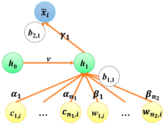
Figure 11. A recurrent neural network with one timestamp for estimating longitudes.

Figure 12. A recurrent neural network with one timestamp for estimating latitudes.

Table 3. The average errors of estimated locations by the proposed mobile positioning method (unit: meters).

Number of Timestamps	Only Cellular Networks	Only Wi-Fi Networks	Cellular and Wi-Fi Networks
1	34.61	16.46	14.39
2	259.44	255.87	252.53
3	254.85	256.61	253.85

4.3.3. Computation Time

For the analyses of computation time, a server with a GPU module (i.e., GeForce GTX 1080) was selected and used. The deep learning models were implemented and executed in TensorFlow and Keras libraries.

In the training stage, the number of epochs was 20,000 for each case. Table 4 showed that the lower computation time was needed for the proposed method with cellular networks (i.e., 59 base stations). The higher computation time was required in the case of cellular and Wi-Fi networks (i.e., 59 base stations and 582 Wi-Fi APs). The computation times of the proposed method with one timestamp (i.e., a neural network) in the cases of cellular networks, Wi-Fi networks, and cellular and Wi-Fi networks were 3022 s, 6928 s, and 7302 s, respectively. In recurrent neural networks, the higher computation time was required for the analyses of time series data. The experimental results showed that the computation times of the proposed method with two and three timestamps in the case of cellular and Wi-Fi networks were 14,533 s and 20,485 s, respectively.

Table 4. The computation time of estimated locations by the proposed mobile positioning method in training stage (unit: seconds).

Number of Timestamps	Only Cellular Networks	Only Wi-Fi Networks	Cellular and Wi-Fi Networks
1	3022	6928	7302
2	5383	13,513	14,533
3	6156	17,938	20,485

In the performing stage, Table 5 showed that the computation times of the proposed method with one, two, and three timestamps in the case of cellular and Wi-Fi networks were 0.37 s, 0.73 s, and 1.02 s, respectively. The precise location information can be quickly obtained by the proposed method with two timestamps.

Table 5. The computation time of estimated locations by the proposed mobile positioning method in performing stage (unit: seconds).

Number of Timestamps	Only Cellular Networks	Only Wi-Fi Networks	Cellular and Wi-Fi Networks
1	0.15	0.35	0.37
2	0.27	0.68	0.73
3	0.31	0.90	1.02

4.3.4. Power Consumption

For the analyses of power consumption, an Android phone (i.e., Redmi 5 running Android platform 7.1.2) was selected and used for measuring its battery life as an indicator. In experiments, an Android application was implemented on the phone to periodically obtain location by GPS or the proposed mobile positioning method. However, the cellular network module was necessarily enabled for data communications via LTE networks. The experimental results were collected and summarized in Table 6. Suppose the battery had a capacity of J Joules. The baseline lifetime with an enabled cellular network module is 254,500 s, so the baseline power consumption B = J/254,500 Watts. For the analysis of Wi-Fi power consumption W, the lifetime with an enabled Wi-Fi module is 175,450 s, so W + B = J/175,450. Furthermore, the lifetime with an enabled GPS module is 81,000 s, so G + B = J/81,000 for the analysis of GPS power consumption G. For the comparison of power consumption, the values of G/B, G/W, and G/(W + B) can be measured as 2.14, 4.75, and 1.47, respectively. Therefore, the proposed method can obtain location information with lower power consumption.

Table 6. The power consumption comparisons. GPS—global positioning system.

Enable Modules	Sampling Period	Lifetime (Seconds)
Cellular	Continuous (1/s)	254,500
Cellular and Wi-Fi	Continuous (1/s)	175,450
Cellular and GPS	Continuous (1/s)	81,000

5. Conclusions and Future Work

This section summarizes and describes the contributions of this study in Section 5.1. The limitations of the proposed method and future work are presented in Section 5.2.

5.1. Conclusions

In previous studies, cellular-based positioning methods could estimate locations of mobile stations in outdoor environments, but the accuracies of estimated locations may have been lower. Moreover, Wi-Fi-based positioning methods can precisely estimate the locations of mobile stations, but the transmission coverage of Wi-Fi APs is not enough in outdoor environments. Although some studies used convolutional neural networks to extract the features of spatio metrics, temporal data of signals from cellular and Wi-Fi networks were not analyzed for reducing location errors. Therefore, a mobile positioning system and a mobile positioning method based on recurrent neural networks are proposed to analyze the RSSIs from heterogeneous networks, which include cellular networks and Wi-Fi networks. The network signals from heterogeneous networks can be analyzed to improve the accuracies of the estimation of locations. Furthermore, the RSSIs in multiple consecutive timestamps can be adopted in recurrent neural networks for the analyses of time series data and location estimation. In practical experimental environments, the results showed that the average error of location estimation was 9.19 m by the proposed mobile positioning method with two timestamps. Therefore, the proposed system and method can be applied to obtain LBS in outdoor environments.

5.2. Future Work

Although the higher accuracies of estimation locations can be obtained by recurrent neural networks with multiple consecutive timestamps, some overfitting problems may exist. For instance, the higher errors of estimated locations were obtained by recurrent neural networks with three timestamps. Therefore, overfitting solutions of time series data [24] can be investigated to improve the accuracies of estimated locations in the future.

References

- Chen, C.H.; Lin, B.Y.; Lin, C.H.; Liu, Y.S.; Lo, C.C. A green positioning algorithm for Campus Guidance System. Int. J. Mob. Commun. 2012, 10, 119–131. [Google Scholar] [CrossRef]
- Wu, C.; Yang, Z.; Xu, Y.; Zhao, Y.; Liu, Y. Human mobility enhances global positioning accuracy for mobile phone localization. IEEE Trans. Parallel Distrib. Syst. 2015, 26, 131–141. [Google Scholar] [CrossRef]
- Thejaswini, M.; Rajalakshmi, P.; Desai, U.B. Novel sampling algorithm for human mobility-based mobile phone sensing. IEEE Internet Things J. 2015, 2, 210–220. [Google Scholar] [CrossRef]
- Molina, B.; Olivares, E.; Palau, C.E.; Esteve, M. A multimodal fingerprint-based indoor positioning system for airports. IEEE Access 2018, 6, 10092–10106. [Google Scholar] [CrossRef]
- Chen, K.; Wang, C.; Yin, Z.; Jiang, H.; Tan, G. Slide: Towards fast and accurate mobile fingerprinting for Wi-Fi indoor positioning systems. IEEE Sens. J. 2018, 18, 1213–1223. [Google Scholar] [CrossRef]
- Liu, D.; Sheng, B.; Hou, F.; Rao, W.; Liu, H. From wireless positioning to mobile positioning: An overview of recent advances. IEEE Syst. J. 2014, 8, 1249–1259. [Google Scholar] [CrossRef]
- Taniuchi, D.; Liu, X.; Nakai, D.; Maekawa, T. Spring model based collaborative indoor position estimation with neighbor mobile devices. IEEE J. Sel. Top. Signal Process. 2015, 9, 268–277. [Google Scholar] [CrossRef]
- Mok, E.; Cheung, B.K.S. An improved neural network training algorithm for Wi-Fi fingerprinting positioning. ISPRS Int. J. Geo-Inf. 2013, 2, 854–868. [Google Scholar] [CrossRef]
- Chen, C.H.; Lin, J.H.; Kuan, T.S.; Lo, K.R. A high-efficiency method of mobile positioning based on commercial vehicle operation data. ISPRS Int. J. Geo-Inf. 2016, 5, 82. [Google Scholar] [CrossRef]
- Xia, S.; Liu, Y.; Yuan, G.; Zhu, M.; Wang, Z. Indoor fingerprint positioning based on Wi-Fi: An overview. ISPRS Int. J. Geo-Inf. 2017, 6, 135. [Google Scholar] [CrossRef]
- Chen, C.Y.; Yin, L.P.; Chen, Y.J.; Hwang, R.C. A modified probability neural network indoor positioning technique. In Proceedings of the 2012 IEEE International Conference on Information Security and Intelligent Control, Yunlin, Taiwan, 14–16 August 2012. [Google Scholar] [CrossRef]
- Xu, Y.; Sun, Y. Neural network-based accuracy enhancement method for WLAN indoor positioning. In Proceedings of the 2012 IEEE Vehicular Technology Conference, Quebec City, QC, Canada, 3–6 September 2012. [Google Scholar] [CrossRef]
- Zhang, T.; Man, Y. The enhancement of WiFi fingerprint positioning using convolutional neural network. In Proceedings of the 2018 International Conference on Computer, Communication and Network Technology, Wuzhen, China, 29–30 June 2018. [Google Scholar] [CrossRef]
- Zhu, J.Y.; Xu, J.; Zheng, A.X.; He, J.; Wu, C.; Li, V.O.K. WIFI fingerprinting indoor localization system based on spatio-temporal (S-T) metrics. In Proceedings of the 2014 IEEE International Conference on Indoor Positioning and Indoor Navigation, Busan, Korea, 27–30 October 2014. [Google Scholar] [CrossRef]
- Lukito, Y.; Chrismanto, A.R. Recurrent neural networks model for WiFi-based indoor positioning system. In Proceedings of the 2017 IEEE International Conference on Smart Cities, Automation & Intelligent Computing Systems, Yogyakarta, Indonesia, 8–10 November 2017. [Google Scholar] [CrossRef]
- Wang, X.; Gao, L.; Mao, S.; Pandey, S. DeepFi: Deep learning for indoor fingerprinting using channel state information. In Proceedings of the 2015 IEEE Wireless Communications and Networking Conference, New Orleans, LA, USA, 9–12 March 2015. [Google Scholar] [CrossRef]
- 3rd Generation Partnership Project. Technical Specification Group Services and System Aspects. Location Services (LCS); Service Description; Stage 1 (Release 15). 2018. Available online: https://portal.3gpp.org/desktopmodules/Specifications/SpecificationDetails.aspx?specificationId=584 (accessed on 23 November 2018).
- Khatab, Z.E.; Hajihoseini, A.; Ghorashi, S.A. A fingerprint method for indoor localization using autoencoder based deep extreme learning machine. IEEE Sens. Lett. 2018, 2, 6000204. [Google Scholar] [CrossRef]
- Wang, X.; Gao, L.; Mao, S.; Pandey, S. CSI-based fingerprinting for indoor localization: A deep learning approach. IEEE Trans. Veh. Technol. 2017, 66, 763–776. [Google Scholar] [CrossRef]
- Wang, X.; Gao, L.; Mao, S. CSI phase fingerprinting for indoor localization with a deep learning approach. IEEE Internet Things J. 2016, 3, 135. [Google Scholar] [CrossRef]
- Shao, W.; Luo, H.; Zhao, F.; Ma, Y.; Zhao, Z.; Crivello, A. Indoor positioning based on fingerprint-image and deep learning. IEEE Access 2018. [Google Scholar] [CrossRef]
- Xiao, C.; Yang, D.; Chen, Z.; Tan, G. 3-D BLE Indoor localization based on denoising autoencoder. IEEE Access 2017, 5, 12751–12760. [Google Scholar] [CrossRef]
- LeCun, Y.; Bengio, Y.; Hinton, G. Deep learning. Nature 2015, 521, 436–444. [Google Scholar] [CrossRef] [PubMed]
- Chen, C.H. Reducing the dimensionality of time-series data with deep learning techniques. Science 2018. Available online: http://science.sciencemag.org/content/313/5786/504/tab-e-letters (accessed on 10 October 2018).
© 2019 by the authors. Licensee MDPI, Basel, Switzerland. This article is an open access article distributed under the terms and conditions of the Creative Commons Attribution (CC BY) license (http://creativecommons.org/licenses/by/4.0/).