Article

Efficient Large Sparse Arrays Synthesis by Means of Smooth Re-Weighted L1 Minimization

by
Daniele Pinchera
1,2,*,
Marco Donald Migliore
1,2,
Mario Lucido
1,2,
Fulvio Schettino
1,2 and
Gaetano Panariello
1,2
1
DIEI, University of Cassino and Southern Lazio, via G. Di Biasio 43, 03043 Cassino, Italy
2
ELEDIA@UniCAS, via G. Di Biasio 43, 03043 Cassino, Italy
*
Author to whom correspondence should be addressed.
Electronics 2019, 8(1), 83; https://doi.org/10.3390/electronics8010083
Submission received: 2 November 2018 / Revised: 20 December 2018 / Accepted: 8 January 2019 / Published: 11 January 2019
(This article belongs to the Special Issue Intelligent Antennas)

Abstract

:
In this paper, we present an efficient technique for the synthesis of very large sparse arrays, with arbitrary circularly-symmetrical upper bounds for the pattern specifications. The algorithm, which is based on iterative smooth re-weighted L1 minimizations, is very flexible and is capable of achieving very good performances with respect to competitive algorithms. Furthermore, thanks to its efficiency, planar arrays of hundreds of wavelengths can be synthesized with limited computational effort.

Graphical Abstract

1. Introduction

Antenna arrays are one of the most important technologies that allows responding to the challenges of the close future communication systems, particularly in the 5G and IoT frameworks [1,2,3,4]. In this perspective, the use of sparse, non-regular, arrays is particularly appealing, since it has been shown that a sparse array is often capable of achieving the same performance of regular lattice ones, with a much lower number of radiating elements, and a strong reduction of the issue of grating lobes.
Unfortunately, the synthesis of a sparse array is a much tougher task with respect to the synthesis of regular lattice ones. This difference is due to the fact that the relationship between the radiated field and the excitation of the radiating elements is linear. This allows the use of efficient linear and convex programming techniques for the determination of the elements’ excitation once the position of the radiators is fixed. Instead, the relationship between the radiated field and the element’s positions is non-linear and non-convex, and no optimal algorithms capable of solving this problem are currently known.
In the last few decades, researchers have followed different approaches to face the synthesis of sparse arrays. They can be roughly summarized into two main categories. In the first one, we have all evolutionary computation-based methods [5,6,7,8,9,10,11,12,13,14,15,16,17,18,19,20], which exploit the capability of genetic algorithms, particle swarm optimization, and similar techniques to face the multiple minima that arise from the aforementioned non-linearity and non-convexity.
A second category is represented by a number of different approaches in which the general synthesis problem is substituted by a simpler one, which can be faced by means of deterministic techniques [21,22,23,24,25,26,27,28,29,30,31,32,33].
Both approaches show advantages and disadvantages. The former class is advantaged from the fact that a well-designed evolutionary algorithm is capable of asymptotically finding the optimal solution of a given problem. The main issue is represented by the word “asymptotically”. The number of iterations needed to get “close” to the global optimum is an exponential function of the number of unknowns, so it is very hard to deal with evolutionary algorithms when the dimension of the desired array is very large: we get a solution, but it is often impossible to say how close to the optimum we are [34].
For the latter category, instead, the execution is—generally speaking—fast, and we are usually allowed to solve, with relative ease, large problems. However, again, since the starting problem solved is a sub-optimal one, we do not usually obtain the global optimum.
The aforementioned classification is obviously a very simplified one, since the years hybrid and mixed strategies have been presented [35,36,37,38,39,40,41]; furthermore, the recent development of compressive sensing [42], and related algorithms, has provided effective and computationally-efficient algorithms [43,44,45,46,47,48,49,50,51,52,53]. In particular, the synthesis of sparse linear arrays of hundreds of wavelengths was shown in [53], a result that to the best knowledge of the authors is currently unmatched.
The synthesis of planar arrays of more than a hundred of wavelengths is instead an open issue. This kind of problems is computationally very difficult to face, because of the huge number of unknowns, with evolutionary algorithms; no results have been shown in the open literature by using other kinds of algorithms.
In this contribution, we will propose a sub-optimal, yet effective, approach to the solution of this kind of problem, to be used for circularly-symmetric beam pattern specifications. In particular, the circular symmetry of the specifications will be used to simplify the layout: we will look for antenna arrays with the elements displaced in circular concentric rings, with a reduction of the number of unknowns to optimize for. Furthermore, we will exploit a smooth re-weighted 1 -norm minimization, a compressive sensing-inspired approach, to look for the minimum number of rings; finally, each ring will be populated with a number of elements as small as possible, to achieve an overall minimum number of radiators.
The paper will be organized as follows. First of all, we will discuss the synthesis problem formulation (Section 2), then we will propose the use of a compressive sensing-like approach for the determination of the number of rings (Section 3) and the population of rings with radiating elements (Section 4). In Section 5, we will provide some numerical results to validate the proposed approach; and conclusions follow (Section 6).

2. Problem Formulation

For the sake of simplicity, we will consider the case of isotropic radiators; most of the considerations that we will discuss in the remainder of the paper can be extended to cases in which we take into account the element factor with minimum effort.
Let us now consider the array factor of N number of sources placed on the { x , y } plane:
F ( θ , ϕ ) = n = 1 N a n e j β ( x n sin θ cos ϕ + y n sin θ sin ϕ )
where β = 2 π / λ is the free space wavenumber, λ is the wavelength, { x n , y n } are the coordinates of the n-th radiating element, and a n is its excitation
The sparse array synthesis problem consists of finding the position and excitation of the N radiating elements in order to satisfy a chosen array factor specification. As an example, we could require that:
| F ( θ , ϕ ) | M U P ( θ , ϕ )
F ( 0 , 0 ) = 1
which represent the typical specifications of a pattern with arbitrary upper bounds.
Some considerations are now in order. First, the number N of radiators could not be specified, and it could also be one of the outputs of the optimization, since such a number is often required to be as small as possible. Second, in some specific applications, we would like all the radiating elements to share the same excitations (i.e., “uniform excitation” arrays) or we suppose that the power delivered to each radiator, which could be also of two or more different kinds, is equal (i.e., “isophoric” arrays).
As stated in the Introduction, the general solution of this kind of problem, even in the case of convex constraints for the pattern specifications, leads to a non-linear and non-convex problem, which is usually very hard to solve, and no deterministic techniques for its optimal solution are known.
It is now worth recalling that, when the array elements are arranged into circles, equally-spaced along each ring (Figure 1), the array factor (1) can be recast in a very convenient way:
F ( θ , ϕ ) = p = 1 P A p N p m = + J m N p ( β R p sin θ ) e j m N p Ξ ( θ , ϕ )
where P is the overall number of rings, N p is the number of antennas along the p-th ring, A p is the common excitation of the elements belonging to the p-th ring of radius R p , J h ( ) is the n-th order Bessel function of the first kind, and Ξ ( θ , ϕ ) is a function of the angular variables, inessential for our purposes [54].
The main advantage of the Formulation (4) is due to the fact that the Bessel functions, other than the zero-order ones, tend to become very small under very simple conditions; in particular, it is well known that | J a ( b ) | < < 1 when b < < a , so looking to the worst case of m = 1 if:
β R p sin θ < < N p 2 π R p / d
where d is the distance between two radiating elements on the same ring. Recasting (5) gives:
d < < λ / sin θ
This means that as long as the elements belonging to the same ring are not too widely spaced, the array factor can be conveniently approximated by:
F ( θ , ϕ ) F ( θ ) = p = 1 P A p N p J 0 ( β R p sin θ )
This approximation is particularly useful, since the synthesis can be done analyzing the θ angular direction only, with a significant computational improvement. Obviously, this simplification is applicable only to the synthesis of a radiation pattern with a circular symmetry (i.e., M U P ( θ , ϕ ) = M U P ( θ ) ).
In the next section, we will discuss how we can use a compressive sensing approach to synthesize very large sparse arrays exploiting (7).

3. Smooth Re-Weighted L1 Minimization

For the sake of simplicity, in the next section, we will call e p = A p N p the ring excitation. The synthesis problem will be then recast as finding the number of rings, their radii, and excitations in order to satisfy the given pattern specifications; the choice of the balancing between A p and N p will depend on the antenna architecture specifications (i.e., constant excitation A p for isophoric arrays).
Let us now consider a dummy ring array, made of a huge number of closely-spaced rings, introducing a dense equispaced position ν -element vector r ˜ in the range [ 0 , R ] , with an inter-element spacing δ much smaller than the wavelength λ , and a vector of observation points w = { w 1 , w ζ } [ 0 , w m a x ] , so that:
F = A e ˜
provides the relationship between the array factor sampled in w h = sin θ h and the vector of ring excitations e ˜ , achieved by the radiation matrix A , whose h , k element is a h , k = J 0 ( β r k w h ) .
The radial and angular discretization of the array factor allow us to solve the synthesis problem by solving the following constrained minimization:
m i n i m i z e e ˜ 0
s u b j e c t t o | A e ˜ | M U P
A 0 e ˜ = 1
where v 0 represents the so-called 0 -norm of v vector, M U P is the sampled version of the upper mask, and A 0 is the array factor in the direction of the desired maximum of the main beam. The p norm of v is defined for p 1 as v p = ( k | v k | p ) 1 / p . Strictly speaking, the so-called 0 -norm is not a norm, and it is given by the number of non-null elements of v .
Once this minimization is solved, the sparse vector of the solution will give us the radii and excitations of the rings of our sparse array (2) and (3). In particular, this approach would lead to the layout employing the smallest number of rings.
Unfortunately, there are no known deterministic optimal techniques to solve the 0 -norm minimization, but as shown in [45,52,55,56], the 0 -norm minimization can be conveniently approximated in a computationally-efficient way by using a sequence of weighted 1 minimizations. We could then try to solve the following convex problem iteratively:
m i n i m i z e g p e ˜ p 1
s u b j e c t t o | A e ˜ p | < M U P
A 0 e ˜ p = 1
where g p e ˜ p is the Hadamard entry-wise product of the two vectors g p and e ˜ p , v 1 is the 1 -norm of the v vector, given by k | v k | , p is the iteration index, and g p = [ g 1 p , , g ν p ] is a proper weighting vector.
As shown in [52], by means of a non-local, “smooth” weighting vector, it is possible to reduce the step of the radial discretization, preserving the small “clusters” that arise in the solution of the 1 -norm minimization. In particular, we have used:
g k p = 1 max ( z k p 1 , η )
where z ˜ p 1 = [ z 1 p 1 , , z ν p 1 ] and:
z ˜ p 1 = | e ˜ p 1 | d
and d is a smoothing vector of positive numbers, while the convolution “*” returns only the central part of it, of the same size as | e ˜ p 1 | .
Once the algorithm has reached a satisfactory solution, it is very easy to extract the ring radii R p and excitations e p from vector e ˜ , by means of the refined clustering approach described in [52].
One of the further advantages of the smooth re-weighted minimization is that, when the iterations have converged (i.e., e ˜ p = e ˜ p 1 ), if some easy conditions are verified [52], we have that:
g p e ˜ p 1 N c
where N c is the number of clusters of non-null elements of e ˜ p , i.e., the number of rings of the sparse concentric ring array synthesized. It should be underlined that, because of the non-convex nature of the synthesis problem, the iterative algorithm could not reach the absolute minimum value of N c (even if it is among one of the possible solutions of the algorithm), since it could stop in a local minimum.
Last but not least, the possibility to reduce the discretization step δ , allowed by the “smooth” weight, is particularly beneficial from a computational point of view, because each 1 minimization iteration requires a computation time that is at least a quadratic function of the number of variables, which is proportional to 1 / δ . This efficiency is numerically confirmed by the quick computation times needed for achieving the results in Section 5.

4. Ring Population from the Calculated Excitation

As stated in Section 2, the ring excitation represents the product of the number of elements and the relative excitation of the radiators belonging to a certain ring. The same ring excitation could be achieved by different combinations of the two factors; the specific choice we need to perform to synthesize the array layout will depend on a particular “ring population strategy”.
In this section, we will discuss two different ring population strategies: the former, to be used in equal amplitude and isophoric arrays; the latter to be used in arrays with variable excitation of the radiating elements.
The key point in both strategies is reducing as much as possible the number of radiators, trying always to limit the effect of the higher order Bessel terms of (4).
For isophoric arrays, we need first to identify the index of the “minimally-populated ring” (MPR), the ring that presents the lowest ratio of the excitation e p and the ring radius R p . Once the MPR has been identified, the number of radiators N M P R on such a ring can be chosen in order to verify:
J N M P R ( β R M P R sin θ ) < T e M P R
where T is a threshold that depends on the required side lobe level (SLL)—usually one hundredth of the SLL is sufficient. The value of N M P R can be determined numerically, and then, the number of radiators on all the other rings can be obtained as:
N p = e p N M P R e M P R
The ring population strategy for arrays with variable elements’ excitation consists, instead, of finding for each ring the minimum number of radiators that allows limiting the effect of higher order Bessel terms:
J N p ( β R p sin θ ) < T e p
Once such a number is found, the element excitation can be achieved by:
A p = e p N p
Obviously, those two strategies aim at the reduction of the number of radiators, and slightly modified versions could be used if other specifications need to be met (for instance, a fixed overall number of radiators). Moreover, the aforementioned strategies can be easily modified to include non-overlapping constraints for the radiators.
The synthesis approach consists of the following steps:
  • Choose the values of δ , d , and η to use.
  • Iteratively solve the problem (12)–(14); usually, less than twenty iterations allow the convergence;
  • we extract the ring radii and excitations from the sparse vector e ˜ ;
  • we populate the ring according to one of the discussed strategies, using (19) or (21).
The core of the procedure is represented by the second step; for convenience of the reader, a simple CVX [57] code implementing the weighted 1 minimization is provided below:
cvx_begin
cvx_solver sedumi
variable e(nu)
minimize (norm (G*e, 1))
subject to
  abs (A*e) <= Mup
  A0*e == 1
cvx_end
In this code, we use SeDuMi as the solver, “e(nu)” is the ν length column vector e ˜ p , “G” is a diagonal matrix implementing the smooth weight (15), “A" and “Mup” are, respectively, the matrix and the column vector implementing (13), and “A0” is a row vector implementing (14).

5. Numerical Examples

In this section, we will provide some examples that will show the effectiveness of the proposed approach. For all the tests, we have used an inter-ring spacing of δ = λ / 20 ; the smoothing vector is d = [ 0.1 , 0.5 , 0.99 , 1 , 0.99 , 0.5 , 0.1 ] , and the tolerance factor is η = max ( | x ˜ p | / 100 ) . All the minimizations have been solved by means of CVX [57] in MATLAB.

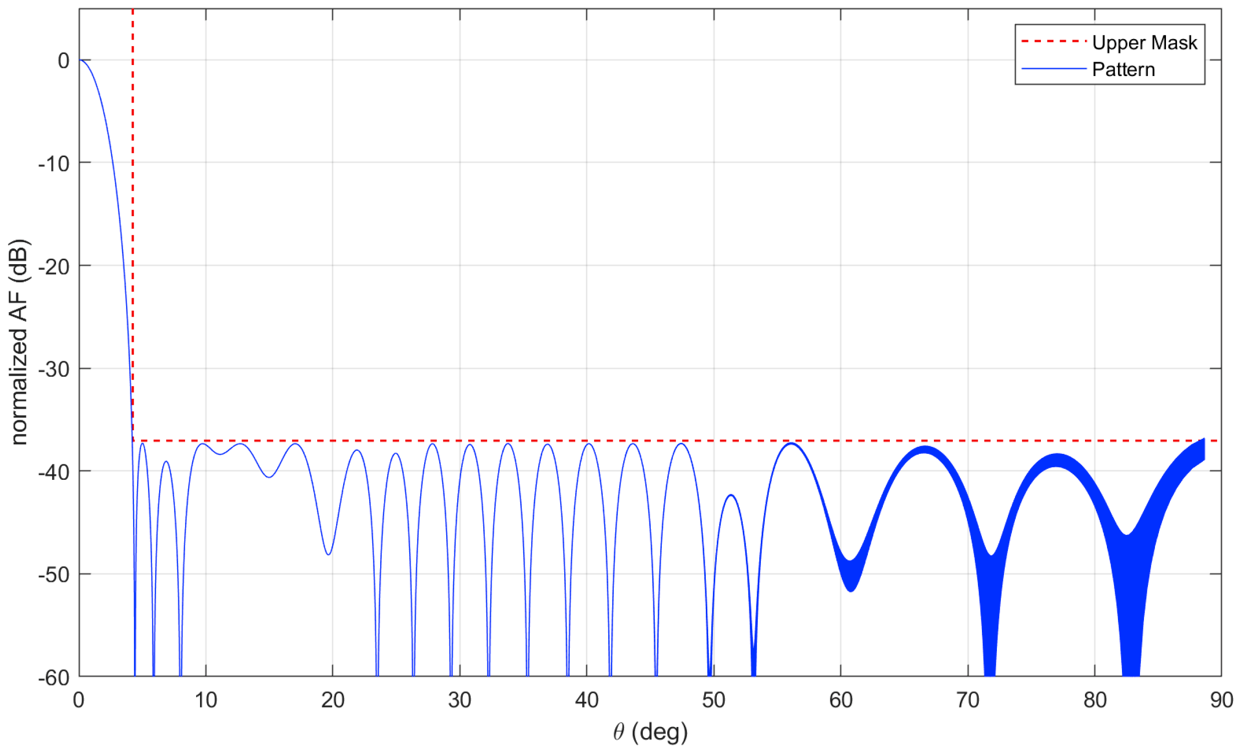
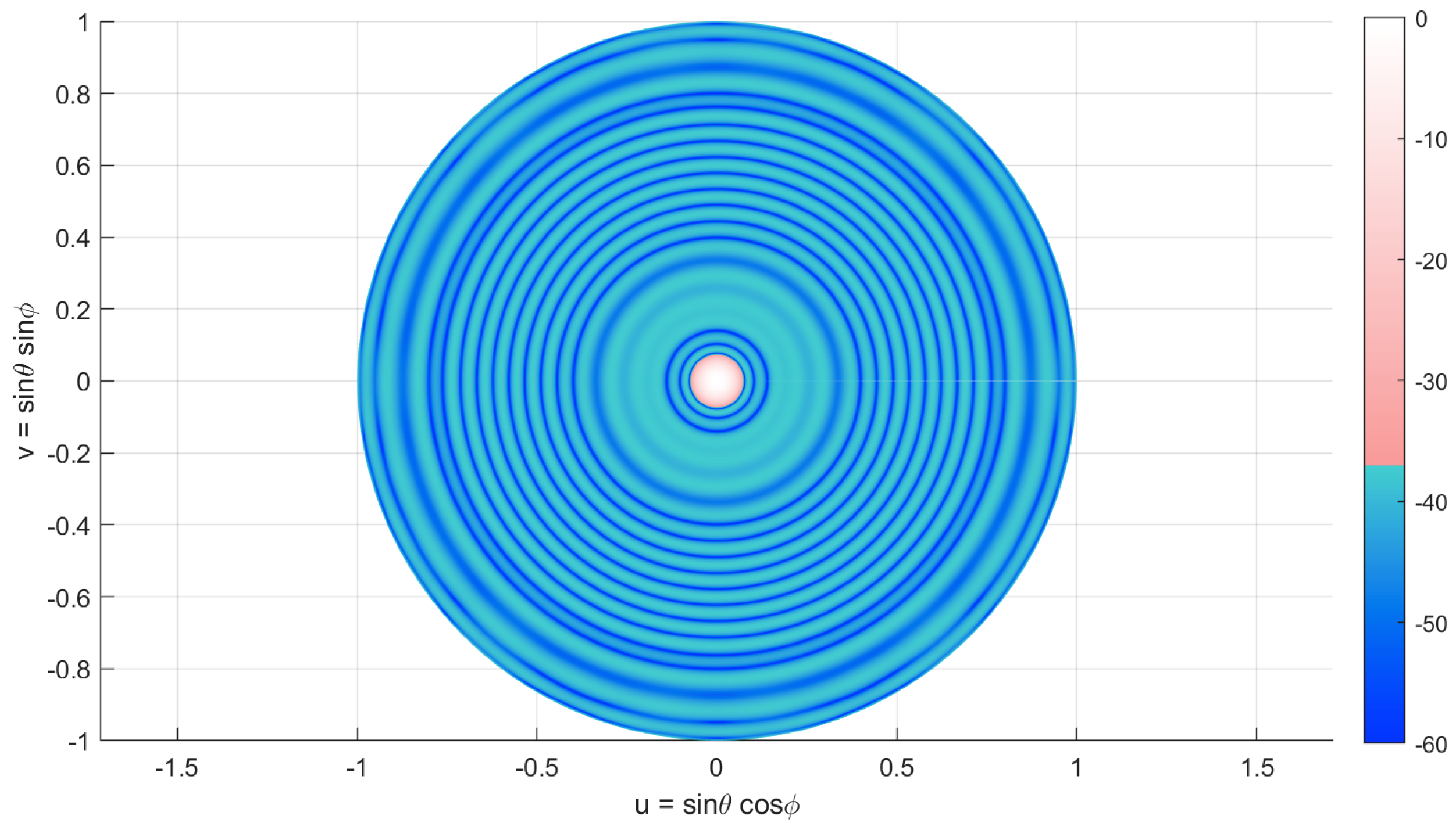
5.1. Large Array with Variable Excitation

In the first example, we will consider the synthesis of a sparse array with the same specification of the 718 elements array of [39]; this sparse array is able to radiate a pattern with a side lobe level lower than −37.05 dB for w 0.074 . By means of the proposed approach, we are able to synthesize a sparse array of 597 elements organized into 12 rings (Figure 2), which satisfies the same specifications with a reduction of the radiating elements’ number of about 17 % with respect to the reference layout.
In particular, the parameters of the found array are provided in Table 1. The minimum, average, and maximum spacing between the rings are, respectively, 0.860 λ , 0.995 λ , and 1.700 λ . The dynamical ratio of the excitations, the ratio of the maximum and minimum excitation of the elements, is 16.5 dB. The array factor of the synthesized array is displayed in Figure 3 and Figure 4. It is interesting to observe from Figure 3 that the ϕ -cuts were perfectly superimposed up to about 56°, confirming the fact that the Bessel function terms other than the zero-order ones are correctly limited by the right choice of the element number per ring.
The calculation of the layout is very quick: ten iterations are needed, and each iteration took about 10 s on an Intel i7 8700k processor.

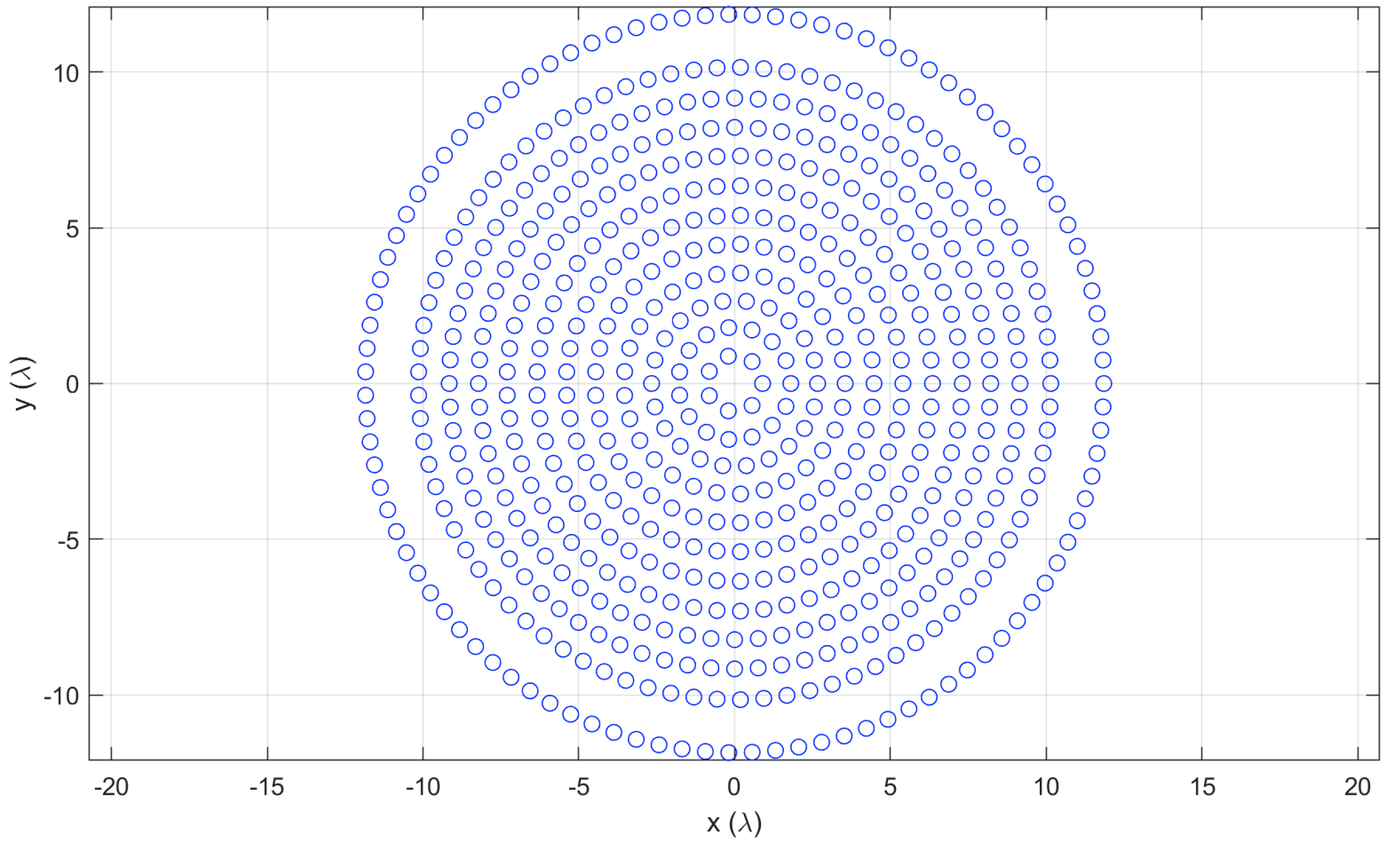
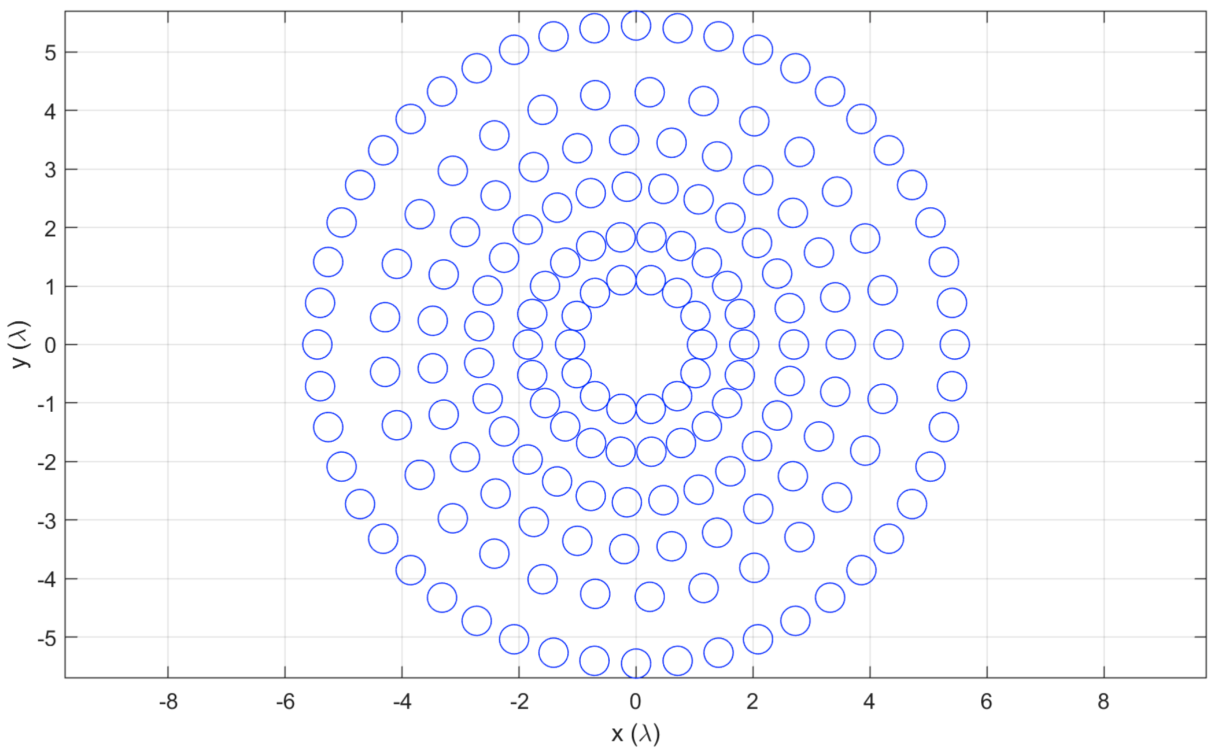
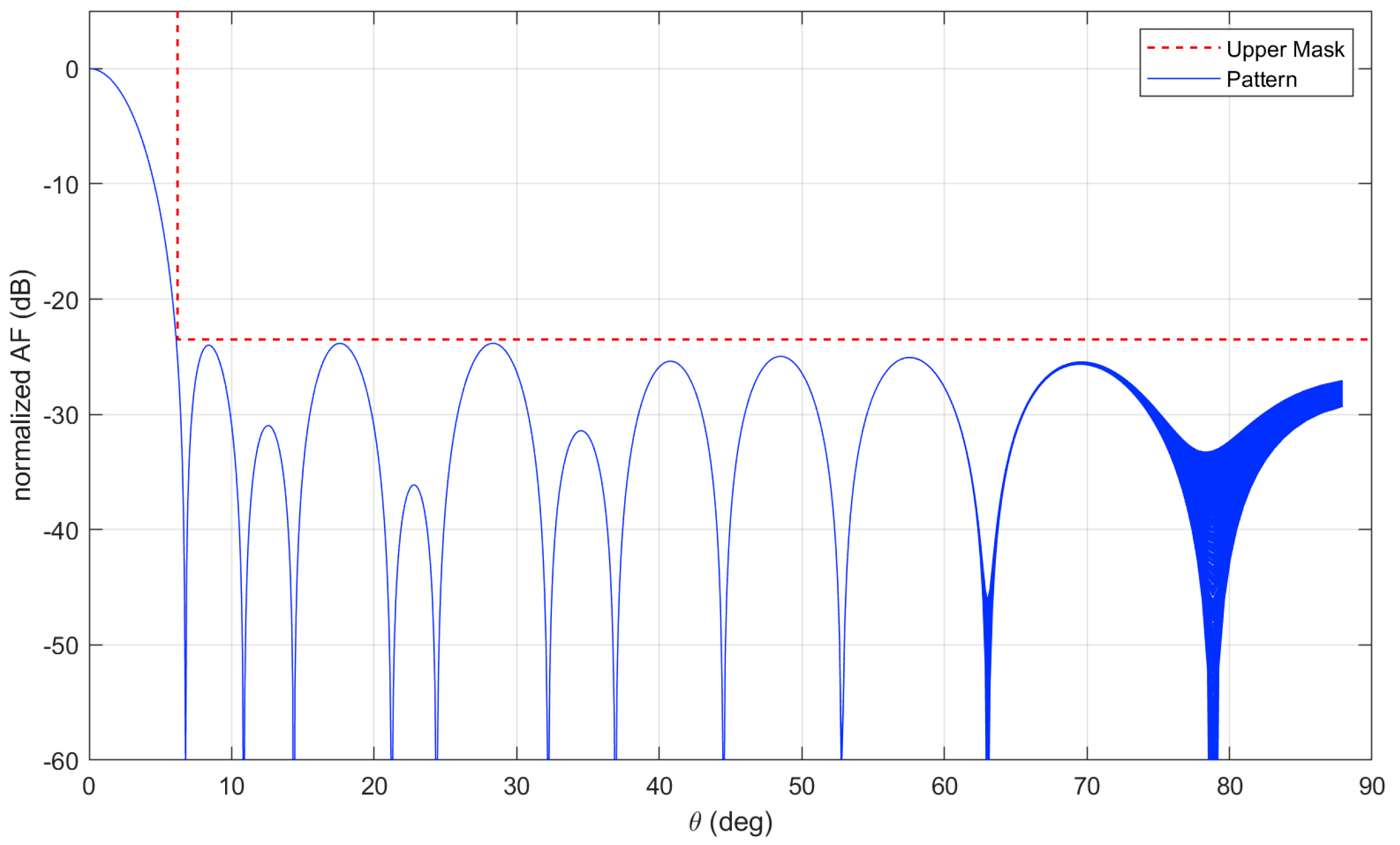
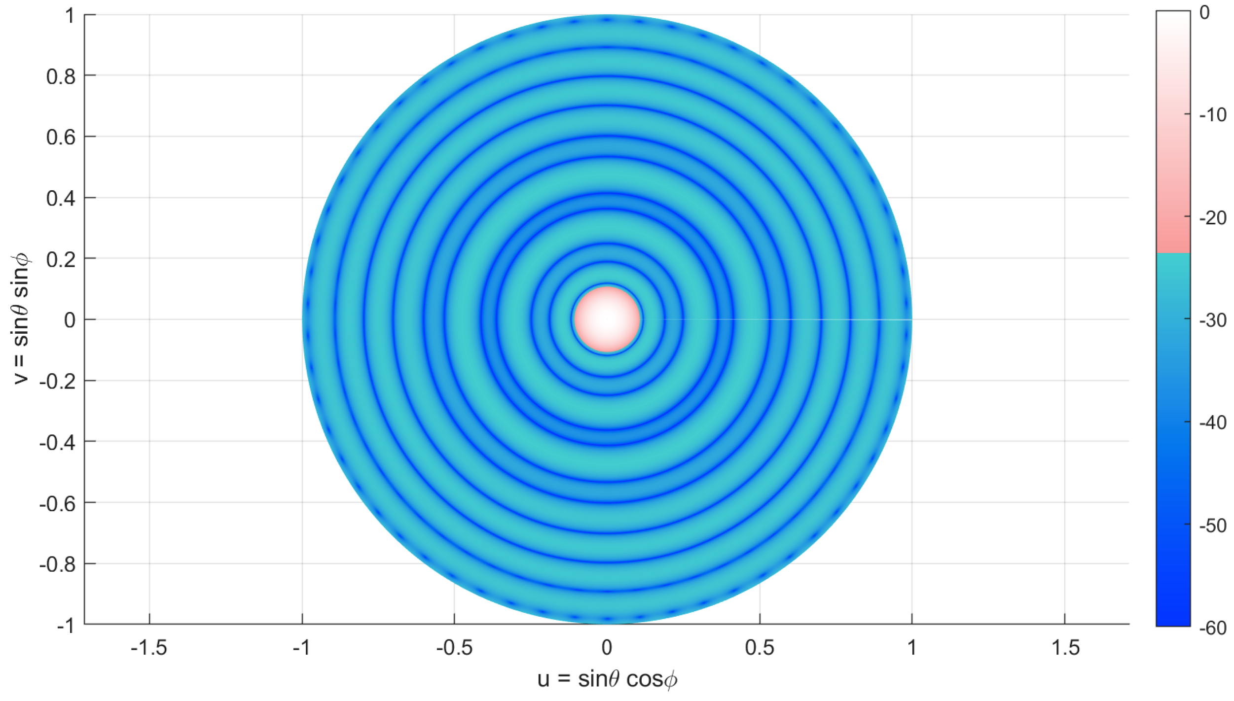
5.2. Small Isophoric Sparse Array

In the second example, we will consider the synthesis of a sparse array with the same specifications of the 185-element array of [51]; this sparse array has been synthesized by means of an approach similar to the one proposed in this paper, but does not employ the smooth weighting function. The reference sparse array is able to radiate a pattern with a side lobe level lower than −23.51 dB and shows a first null beamwidth (FNBW) of 14.2°. By means of our approach, we are able to synthesize a sparse array of 167 elements organized into six rings (Figure 5), which satisfies the same SLL specifications with a reduction of beamwidth (in our case. the FNBW is 13.5°) and a reduction of the radiating element number of about 10 % .
In particular, the parameters of the found array are provided in Table 2. The minimum, average, and maximum spacing between the rings are, respectively, 0.72273 λ , 0.86454 λ , and 1.1333 λ . The array factor of the synthesized array is displayed in Figure 6 and Figure 7.
It is worth noting that the calculation of the layout is almost instantaneous: only three iterations are needed, and each iteration took less than 2 s on an Intel i7 8700k processor.

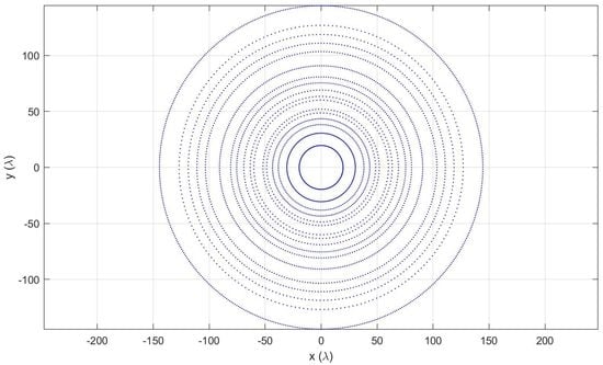
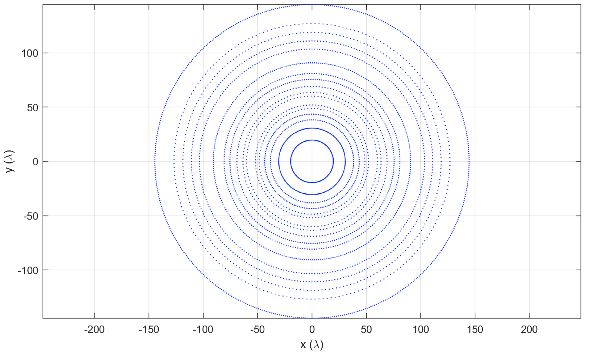
5.3. Very Large Isophoric Sparse Array

In this section, we instead will discuss the synthesis of a large sparse array with constant element excitation, with a diameter of about 290 λ . To the best knowledge of the authors, there are no results available in the open literature with sparse arrays of these dimensions, confirming the capability of the proposed approach to handle synthesis problems of very high size.
The particular array sought should be able to radiate a pencil beam with a side lobe level lower than −30 dB for w 0.005 and to scan it on the whole Earth’s surface from GEO orbit, always satisfying the SLL constraint within the Earth’s surface (that is seen as a solid angle of about 8.5 (deg) radius). For this reason, the synthesis will be performed in the angular region with w m a x = 0.287 , following the guidelines in [31].
By means of the proposed approach, we are able to synthesize a sparse array of 3516 elements organized into 17 rings; see Figure 8, which perfectly satisfies the same chosen specifications.
In particular, the parameters of the found array are provided in Table 3. The minimum, average, and maximum spacing between the rings are, respectively, 3.350 λ , 7.804 λ , and 17.559 λ . The array factor of the synthesized array is displayed in Figure 9 and Figure 10; in Figure 11, we also show a scanned beam at the edge of the Earth’s surface, as seen from GEO orbit.
In this case, the calculation of the layout is slower than the previous cases: 41 iterations are needed, and each iteration took about 70 s on an Intel i7 8700k processor; but considering the dimension of the achieved layout, this is indeed an excellent result.

6. Discussion and Conclusions

A very efficient algorithm for the synthesis of sparse arrays has been presented.
The approach is capable of synthesizing sparse arrays with variable or constant excitation of the elements, allowing the satisfaction of circularly-symmetrical constraints for the upper bounds of the pattern.
The results shown, summarized in Table 4, are very good, and the obtained layouts present a lower number of elements with respect to other algorithms in the literature, when the same pattern specifications are met. Obviously, we do not believe that our algorithm is able to provide the best solutions, since the problem it solves is just an approximation of the more general synthesis problem. Accordingly, the method does not assure the optimality of the solution.
It is worth noting that, due to the complex non-linear characteristic of the synthesis problem object of the paper, no method (including genetic algorithms) assures the convergence toward the optimal solution in finite time. Furthermore, the radiators are “forced” into concentric rings, instead of being freely placed on a plane. However, the good quality of the results obtained, together with the relative quickness of the method even for very large arrays, make us confident of the significance of our approach.
It has also to be underlined that the computational efficiency of the approach allows to face also problems of very large size: in one of the examples a sparse planar array of about three hundred wavelengths is demonstrated, and in other numerical tests, not shown here for sake of brevity, we were able to synthesize even larger arrays.
In a future development we plan to extend the proposed synthesis method to the case of shaped beams.

Author Contributions

D.P., M.D.M. and G.P. conceived the method; D.P. wrote the numerical code and performed the array syntheses; M.D.M., M.L. and F.S. helped with the comparison with other approaches; D.P., G.P., F.S. and M.D.M. wrote the paper.

Funding

This paper has been supported by the MIUR program “Dipartimenti di Eccellenza 2018–2022”.

Conflicts of Interest

The authors declare no conflict of interest.

References

  1. Weber, R.H.; Weber, R. Internet of Things; Springer: Berlin, Germany, 2010; Volume 12. [Google Scholar]
  2. Pinchera, D.; Migliore, M.D.; Schettino, F.; Panariello, G. Antenna Arrays for Line-of-Sight Massive MIMO: Half Wavelength Is Not Enough. Electronics 2017, 6, 57. [Google Scholar] [CrossRef]
  3. Larsson, E.G.; Edfors, O.; Tufvesson, F.; Marzetta, T.L. Massive MIMO for next generation wireless systems. IEEE Commun. Mag. 2014, 52, 186–195. [Google Scholar] [CrossRef] [Green Version]
  4. Zhao, D.; Jin, T.; Dai, Y.; Song, Y.; Su, X. A Three-Dimensional Enhanced Imaging Method on Human Body for Ultra-Wideband Multiple-Input Multiple-Output Radar. Electronics 2018, 7, 101. [Google Scholar]
  5. Haupt, R.L. Thinned arrays using genetic algorithms. IEEE Trans. Antennas Propag. 1994, 42, 993–999. [Google Scholar] [CrossRef]
  6. Trucco, A.; Omodei, E.; Repetto, P. Synthesis of sparse planar arrays. Electron. Lett. 1997, 33, 1834–1835. [Google Scholar] [CrossRef]
  7. Bray, M.G.; Werner, D.H.; Boeringer, D.W.; Machuga, D.W. Optimization of thinned aperiodic linear phased arrays using genetic algorithms to reduce grating lobes during scanning. IEEE Trans. Antennas Propag. 2002, 50, 1732–1742. [Google Scholar] [CrossRef]
  8. Migliore, M.D.; Pinchera, D.; Schettino, F. A simple and robust adaptive parasitic antenna. IEEE Trans. Antennas Propag. 2005, 53, 3262–3272. [Google Scholar] [CrossRef]
  9. Chen, K.; He, Z.; Han, C.C. A modified real GA for the sparse linear array synthesis with multiple constraints. IEEE Trans. Antennas Propag. 2006, 54, 2169–2173. [Google Scholar] [CrossRef]
  10. Quevedo-Teruel, O.; Rajo-Iglesias, E. Ant colony optimization in thinned array synthesis with minimum sidelobe level. IEEE Antennas Wirel. Propag. Lett. 2006, 5, 349–352. [Google Scholar] [CrossRef]
  11. Migliore, M.D.; Pinchera, D.; Schettino, F. Improving Channel Capacity Using Adaptive MIMO Antennas. IEEE Trans. Antennas Propag. 2006, 54, 3481–3489. [Google Scholar] [CrossRef]
  12. Haupt, R.L. Optimized element spacing for low sidelobe concentric ring arrays. IEEE Trans. Antennas Propag. 2008, 56, 266–268. [Google Scholar] [CrossRef]
  13. Reyna, A.; Panduro, M.A.; Del Rio, C. Design of concentric ring antenna arrays for isoflux radiation in GEO satellites. IEICE Electron. Express 2011, 8, 484–490. [Google Scholar] [CrossRef]
  14. Goudos, S.K.; Siakavara, K.; Samaras, T.; Vafiadis, E.E.; Sahalos, J.N. Sparse linear array synthesis with multiple constraints using differential evolution with strategy adaptation. IEEE Antennas Wirel. Propag. Lett. 2011, 10, 670–673. [Google Scholar] [CrossRef]
  15. Cen, L.; Yu, Z.L.; Ser, W.; Cen, W. Linear aperiodic array synthesis using an improved genetic algorithm. IEEE Trans. Antennas Propag. 2012, 60, 895–902. [Google Scholar] [CrossRef]
  16. Zhang, L.; Jiao, Y.C.; Chen, B. Optimization of concentric ring array geometry for 3D beam scanning. Int. J. Antennas Propag. 2012, 2012, 625437. [Google Scholar] [CrossRef]
  17. Manica, L.; Anselmi, N.; Rocca, P.; Massa, A. Robust mask-constrained linear array synthesis through aninterval-based particle SWARM optimisation. IET Microw. Antennas Propag. 2013, 7, 976–984. [Google Scholar] [CrossRef]
  18. Chen, K.; Chen, H.; Wang, L.; Wu, H. Modified real ga for the synthesis of sparse planar circular arrays. IEEE Antennas Wirel. Propag. Lett. 2016, 15, 274–277. [Google Scholar] [CrossRef]
  19. Jiang, Y.; Zhang, S.; Guo, Q.; Li, M. Synthesis of uniformly excited concentric ring arrays using the improved integer GA. IEEE Antennas Wirel. Propag. Lett. 2016, 15, 1124–1127. [Google Scholar] [CrossRef]
  20. Polo-López, L.; Córcoles, J.; Ruiz-Cruz, J.A. Antenna Design by Means of the Fruit Fly Optimization Algorithm. Electronics 2018, 7, 3. [Google Scholar] [CrossRef]
  21. Leahy, R.M.; Jeffs, B.D. On the design of maximally sparse beamforming arrays. IEEE Trans. Antennas Propag. 1991, 39, 1178–1187. [Google Scholar] [CrossRef] [Green Version]
  22. Marchaud, F.B.; De Villiers, G.D.; Pike, E.R. Element positioning for linear arrays using generalized Gaussian quadrature. IEEE Trans. Antennas Propag. 2003, 51, 1357–1363. [Google Scholar] [CrossRef]
  23. Liu, Y.; Nie, Z.; Liu, Q.H. Reducing the number of elements in a linear antenna array by the matrix pencil method. IEEE Trans. Antennas Propag. 2008, 56, 2955–2962. [Google Scholar] [CrossRef]
  24. Oliveri, G.; Donelli, M.; Massa, A. Linear array thinning exploiting almost difference sets. IEEE Trans. Antennas Propag. 2009, 57, 3800–3812. [Google Scholar] [CrossRef]
  25. Angeletti, P.; Toso, G. Synthesis of circular and elliptical sparse arrays. Electron. Lett. 2011, 47, 304–305. [Google Scholar] [CrossRef]
  26. Yang, K.; Zhao, Z.; Liu, Y. Synthesis of sparse planar arrays with matrix pencil method. In Proceedings of the 2011 International Conference on Computational Problem-Solving (ICCP), Chengdu, China, 21–23 October 2011; pp. 82–85. [Google Scholar]
  27. Bucci, O.M.; Perna, S.; Pinchera, D. Advances in the deterministic synthesis of uniform amplitude pencil beam concentric ring arrays. IEEE Trans. Antennas Propag. 2012, 60, 3504–3509. [Google Scholar] [CrossRef]
  28. Guo, H.; Guo, C.J.; Qu, Y.; Ding, J. Pattern synthesis of concentric circular antenna array by nonlinear least-square method. Prog. Electromagn. Res. 2013, 50, 331–346. [Google Scholar] [CrossRef]
  29. Oliveri, G.; Bekele, E.T.; Robol, F.; Massa, A. Sparsening Conformal Arrays Through a Versatile-Based Method. IEEE Trans. Antennas Propag. 2014, 62, 1681–1689. [Google Scholar] [CrossRef]
  30. Angeletti, P.; Toso, G.; Ruggerini, G. Array antennas with jointly optimized elements positions and dimensions part II: Planar circular arrays. IEEE Trans. Antennas Propag. 2014, 62, 1627–1639. [Google Scholar] [CrossRef]
  31. Bucci, O.M.; Isernia, T.; Perna, S.; Pinchera, D. Isophoric sparse arrays ensuring global coverage in satellite communications. IEEE Trans. Antennas Propag. 2014, 62, 1607–1618. [Google Scholar] [CrossRef]
  32. Liu, Y.; You, P.; Zhu, C.; Tan, X.; Liu, Q.H. Synthesis of sparse or thinned linear and planar arrays generating reconfigurable multiple real patterns by iterative linear programming. Prog. Electromagn. Res. 2016, 155, 27–38. [Google Scholar] [CrossRef]
  33. Bucci, O.; Perna, S.; Pinchera, D. Interleaved Isophoric Sparse Arrays for the Radiation of Steerable and Switchable Beams in Satellite Communications. IEEE Trans. Antennas Propag. 2017, 65, 1163–1173. [Google Scholar] [CrossRef]
  34. Pinchera, D.; Migliore, M.D. Comparison Guidelines and Benchmark Procedure for Sparse Array Synthesis. Prog. Electromagn. Res. 2016, 52, 129–139. [Google Scholar] [CrossRef]
  35. Caorsi, S.; Lommi, A.; Massa, A.; Pastorino, M. Peak sidelobe level reduction with a hybrid approach based on GAs and difference sets. IEEE Trans. Antennas Propag. 2004, 52, 1116–1121. [Google Scholar] [CrossRef]
  36. Donelli, M.; Caorsi, S.; DeNatale, F.; Pastorino, M.; Massa, A. Linear antenna synthesis with a hybrid genetic algorithm. Prog. Electromagn. Res. 2004, 49, 1–22. [Google Scholar] [CrossRef]
  37. D’Urso, M.; Isernia, T. Solving some array synthesis problems by means of an effective hybrid approach. IEEE Trans. Antennas Propag. 2007, 55, 750–759. [Google Scholar] [CrossRef]
  38. Bucci, O.M.; Pinchera, D. A generalized hybrid approach for the synthesis of uniform amplitude pencil beam ring-arrays. IEEE Trans. Antennas Propag. 2012, 60, 174–183. [Google Scholar] [CrossRef]
  39. Liu, J.; Zhao, Z.; Yang, K.; Liu, Q.H. A hybrid optimization for pattern synthesis of large antenna arrays. Prog. Electromagn. Res. 2014, 145, 81–91. [Google Scholar] [CrossRef]
  40. Bucci, O.M.; Perna, S.; Pinchera, D. Synthesis of isophoric sparse arrays allowing zoomable beams and arbitrary coverage in satellite communications. IEEE Trans. Antennas Propag. 2015, 63, 1445–1457. [Google Scholar] [CrossRef]
  41. Pinchera, D.; Perna, S.; Migliore, M.D. A Lexicographic Approach for Multi-Objective Optimization in Antenna Array Design. Prog. Electromagn. Res. 2017, 59, 85–102. [Google Scholar] [CrossRef]
  42. Baraniuk, R.G. Compressive sensing. IEEE Signal Process. Mag. 2007, 24, 118–121. [Google Scholar] [CrossRef]
  43. Zhang, W.; Li, L.; Li, F. Reducing the number of elements in linear and planar antenna arrays with sparseness constrained optimization. IEEE Trans. Antennas Propag. 2011, 59, 3106–3111. [Google Scholar] [CrossRef]
  44. Oliveri, G.; Massa, A. Bayesian compressive sampling for pattern synthesis with maximally sparse non-uniform linear arrays. IEEE Trans. Antennas Propag. 2011, 59, 467–481. [Google Scholar] [CrossRef]
  45. Fuchs, B. Synthesis of sparse arrays with focused or shaped beampattern via sequential convex optimizations. IEEE Trans. Antennas Propag. 2012, 60, 3499–3503. [Google Scholar] [CrossRef]
  46. Oliveri, G.; Carlin, M.; Massa, A. Complex-weight sparse linear array synthesis by Bayesian compressive sampling. IEEE Trans. Antennas Propag. 2012, 60, 2309–2326. [Google Scholar] [CrossRef]
  47. Carlin, M.; Oliveri, G.; Massa, A. Hybrid BCS-deterministic approach for sparse concentric ring isophoric arrays. IEEE Trans. Antennas Propag. 2015, 63, 378–383. [Google Scholar] [CrossRef]
  48. D’Urso, M.; Prisco, G.; Tumolo, R.M. Maximally Sparse, Steerable, and Nonsuperdirective Array Antennas via Convex Optimizations. IEEE Trans. Antennas Propag. 2016, 64, 3840–3849. [Google Scholar] [CrossRef]
  49. Bencivenni, C.; Ivashina, M.; Maaskant, R.; Wettergren, J. Synthesis of maximally sparse arrays using compressive sensing and full-wave analysis for global earth coverage applications. IEEE Trans. Antennas Propag. 2016, 64, 4872–4877. [Google Scholar] [CrossRef]
  50. Pinchera, D.; Migliore, M.D.; Lucido, M.; Schettino, F.; Panariello, G. A Compressive-Sensing Inspired Alternate Projection Algorithm for Sparse Array Synthesis. Electronics 2017, 6, 3. [Google Scholar] [CrossRef]
  51. Zhao, X.; Yang, Q.; Zhang, Y. A hybrid method for the optimal synthesis of 3-D patterns of sparse concentric ring arrays. IEEE Trans. Antennas Propag. 2016, 64, 515–524. [Google Scholar] [CrossRef]
  52. Pinchera, D.; Migliore, M.D.; Schettino, F.; Lucido, M.; Panariello, G. An Effective Compressed-Sensing Inspired Deterministic Algorithm for Sparse Array Synthesis. IEEE Trans. Antennas Propag. 2018, 66, 149–159. [Google Scholar] [CrossRef]
  53. Pinchera, D.; Migliore, M.D.; Panariello, G. Synthesis of Large Sparse Arrays Using IDEA (Inflating-Deflating Exploration Algorithm). IEEE Trans. Antennas Propag. 2018, 66, 4658–4668. [Google Scholar] [CrossRef]
  54. Balanis, C. Antenna Theory: Analysis and Design; Wiley: New York, NY, USA, 2015. [Google Scholar]
  55. Prisco, G.; D’Urso, M. Maximally sparse arrays via sequential convex optimizations. IEEE Antennas Wirel. Propag. Lett. 2012, 11, 192–195. [Google Scholar] [CrossRef]
  56. Migliore, M.D. On the sampling of the electromagnetic field radiated by sparse sources. IEEE Trans. Antennas Propag. 2015, 63, 553–564. [Google Scholar] [CrossRef]
  57. Grant, M.; Boyd, S. CVX: Matlab Software for Disciplined Convex Programming, Version 2.1. 2014. Available online: http://cvxr.com/cvx (accessed on 10 January 2019).
Figure 1. Scheme of a circular concentric ring array.
Electronics 08 00083 g001
Figure 2. Layout of the 597-element sparse array. Each radiator is represented by a circle of half a wavelength diameter.
Electronics 08 00083 g002
Figure 3. Plot of the ϕ -cuts of the array factor for the 597-element array.
Electronics 08 00083 g003
Figure 4. Imagemap of the array factor in the u , v plane for the 597-element array. The dual tone (pink/cyan) colormap does not show any violation of the SLL constraint out of the main beam.
Electronics 08 00083 g004
Figure 5. Layout of the 167-element sparse array. Each radiator is represented by a circle of half a wavelength diameter.
Electronics 08 00083 g005
Figure 6. Plot of the ϕ -cuts of the array factor for the 167-element array.
Electronics 08 00083 g006
Figure 7. Imagemap of the array factor in the u , v plane for the 167-element array. The dual tone (pink/cyan) colormap does not show any violation of the SLL constraint out of the main beam.
Electronics 08 00083 g007
Figure 8. Layout of the 3516-element sparse array. Each radiator is represented by a circle of half a wavelength diameter.
Electronics 08 00083 g008
Figure 9. Plot of the ϕ -cuts of the array factor for the 3516-element array.
Electronics 08 00083 g009
Figure 10. Imagemap of the array factor for the broadside beam in the u , v plane for the 3516-element array. Only the inner part of the u , v plane, relative to Earth’s surface as seen from GEO orbit is displayed.
Electronics 08 00083 g010
Figure 11. Imagemap of the array factor for the beam scanned to 8° deg in the u , v plane for the 3516 element array. Only the inner part of the u , v plane, relative to the Earth’s surface as seen from GEO orbit, is displayed. The dual tone (pink/cyan) colormap does not show any violation of the SLL constraint out of the main beam.
Electronics 08 00083 g011
Table 1. Parameters of the synthesized 597 element array.
# R p ( λ ) N p A p
10.970.693
21.805151
32.665220.943
43.55290.794
54.476370.72
65.403450.631
76.352530.52
87.309610.464
98.222680.368
109.161760.269
1110.15850.277
1211.85990.15
Table 2. Parameters of the synthesized 167-element array.
# R p ( λ ) N p
11.12714
21.8522
32.727
43.527
54.31729
65.4548
Table 3. Parameters of the synthesized 3516-element array.
# R p ( λ ) N p
119.602144
230.594192
338.25139
443.45167
548.647103
652117
760.1119
863.45130
969.048162
1075.5238
1180.84232
1290.75301
13103.45272
14110.95264
15118.721223
16126.9215
17144.459498
Table 4. Results’ summary. FNBW, first null beamwidth.
LayoutNMain BeamSLL (dB)IterationsIteration Time (s)
Figure 2597 w 0.074 −37.051010
Ref. [39]718 w 0.074 −37.05n.a.n.a.
Figure 5167FNBW = 13.5°−23.5132
Ref. [51]185FNBW = 14.2°−23.51n.a.n.a.
Figure 83516 w 0.005 −304170
Computation times refer to an i7 8700k PC.

