Harmonic PMU Algorithm Based on Complex Filters and Instantaneous Single-Sideband Modulation

Abstract

Phasor measurement units (PMUs) have become powerful monitoring tools for many applications in smart grids. In order to address the different issues related to harmonics in power systems, the fundamental phasor estimator in a PMU has been extended to the harmonic phasor estimator by several researchers around the world. Yet, the development of harmonic phasor estimators is a challenge because they have to consider time-varying frequencies since the frequency deviation in the harmonic components is proportional to the harmonic order in a dynamic way. In this work, a new algorithm for harmonic phasor estimation using an instantaneous single-sideband (SSB) modulation is presented. Unlike other SSB-based approaches, its implementation in this work is based on concepts of instantaneous phase and instantaneous frequency. In general, the proposed algorithm is divided into two stages. Firstly, the estimation of the fundamental phasor is carried out by means of a complex finite impulse response (FIR) filter which provides the analytic signal used to compute the instantaneous magnitude, phase, and frequency. Secondly, a complex FIR filter bank is proposed for the estimation of the harmonic components, where the instantaneous SSB modulation technique is applied in order to center the harmonic components into specific narrow bands for each complex filter when an off-nominal frequency occurs. The validation of the proposed algorithm is carried out by means of the current standards of phasor measurement units, i.e., Std. C37.118.1-2011 and C37.118.1a-2014, which involve steady-state, dynamic, and time performance tests.

1. Introduction

Proliferation of non-linear loads along with the growth of distributed generation systems are some of the main causes of power quality problems related to harmonic pollution in modern power systems [1]. This pollution compromises the system reliability, e.g., producing additional losses in transmission or distribution lines, overheating of electrical machines and relays breakdowns [2,3]. At the same time, the development of new power system topics, such as smart grids and renewable energies, increases the requirements of methodologies for power quality monitoring [4,5,6,7], including the analysis of both the fundamental component and the harmonic components [8]. Regarding the fundamental component, phasor measurement units (PMUs) are synchronized remote devices commonly used for wide area monitoring systems with high performance requirements for phasor, frequency and rate of change of frequency (ROCOF) errors defined in the current standard, i.e., the IEEE Std. C37.118.1-2011 and -2014 [9,10,11]. Although PMU standards are set originally for fundamental component measurements according to the required performance: P class or M class, their benchmark tests and requirements can be extended to harmonic components for validation purposes [9]. Therefore, a PMU with capabilities for harmonic estimation will allow improving the performance in different applications of power systems such as power quality monitoring, adaptive protections, network reconfiguration under fault conditions, and so on [12].

In literature, different algorithms for estimation of both fundamental phasor and harmonic phasor have been reported. Among the algorithms for the former [13,14,15], the Fourier transform (FT) has been widely used; however, it presents some drawbacks that compromise its performance, e.g., the assumption of periodic signals, spectral leakage produced when the fundamental frequency fluctuates, and that the frequency resolution depends on the time observation window [16,17]. Regarding the harmonic synchrophasor implementations, few strategies have been presented. For instance, in [2,12], the FT and a zero-crossing technique is used to calculate the fundamental and harmonic components, in which unreliable results can be obtained when a frequency fluctuation appears. In [18], an improved FT version is presented where several windows to reduce the spectral leakage are compared; besides that, it uses a curve fitting approach with fundamental frequency information for estimation of the harmonic phasors. Another work that follows the synchrophasors guidelines is carried out in [19], which proposes an estimator in off-nominal frequency conditions based on a frequency tracking process and a harmonic model, solving the model by means of a singular value decomposition method. Similarly, in [20], a recursive-least-squares technique synchronized by a phase-locked loop (PLL) is proposed. Also, harmonic dynamic models have been proposed and solved using approaches based on Taylor and Kalman filters (KF) [21,22] and a rotational invariance technique [23]. Further, in [9], both the KF and a FIR filter with adaptive filter coefficients as a function of the fundamental frequency for harmonic phasor estimation are presented. From these works, it is evident that the concept of harmonic synchrophasor has been investigated with special attention in the fundamental frequency since, on the one hand, it is used for the harmonic phasor estimations and, on the other hand, it is related to the accuracy of the results [18]. However, these works are leaving out important parameters such as the frequency error (FE) and the rate of change of frequency error (RFE) along with the benchmark tests required in the current synchrophasor standards, which can be taken as reference in order to validate in a more complete way the performance of a harmonic PMU.

In this paper, a new algorithm for phasor estimation of harmonic components in a PMU context is proposed. This algorithm is based on a complex brick-wall band-pass FIR filter for the estimation of both the fundamental phasor and the fundamental frequency. The harmonic phasors are estimated using a complex FIR filter bank by centering the harmonic components of the signal according to its frequency deviation by means of an instantaneous single-sideband (SSB) modulation technique. This technique allows shifting the spectral content of the signal using a Hilbert filter and a complex modulation process using the instantaneous frequency deviation. In this regard, the proposed algorithm represents a new scheme for harmonic estimation in a PMU context with a low-complex technique. The proposed algorithm is evaluated under all the steady-state and dynamic conditions established in the IEEE Std. C37.118.1-2011 [10] along with its amendment C37.118.1a-2014 [11]. These conditions are amplitude, phase and frequency variations, total harmonic distortion (THD), out-of-band interference, amplitude and phase modulations, frequency ramp, amplitude and phase steps. Besides that, unlike other proposals, even and odd harmonic components are analyzed for each condition. Then, the total vector error (TVE), FE, and RFE parameters, which are extended to the harmonic components, are analyzed according to the allowable limits for the M class. This class is chosen since the proposal is oriented to applications that require higher levels of accuracy and has to satisfy the out-of-band interference test which is one of the most challenging tests. The results show the feasibility of the proposed method for harmonic synchrophasor applications, where a complete fulfillment of the benchmark tests is obtained.

2. Theoretical Background

2.1. Harmonic Phasor Model

PMUs provide a synchronized magnitude and phase estimation under a coordinated universal time (UTC) of an electric signal [24,25]. This signal is determined by:

$$x(t)=\frac{A}{\sqrt{2}}\cos (2\pi f_{0}t+2\pi {\displaystyle \int \Delta fdt}+\varphi )$$

(1)

where A is the amplitude, f₀ is the nominal system frequency (50 Hz/60 Hz), Δf is the frequency deviation, and ϕ is the phase angle. From (1), the synchrophasor representation is defined as [10]:

$$X(t)=\frac{A}{\sqrt{2}}{e}^{2\pi {\displaystyle \int \Delta fdt}+\varphi }$$

(2)

In the same way, a sinusoidal signal with harmonic content can be expressed as:

$$x(t)={\displaystyle \sum _{h=1}^H\frac{A_h}{\sqrt{2}}\cos (h(2\pi f_{0}t+2\pi {\displaystyle \int \Delta fdt)}+{\varphi }_h)}$$

(3)

where h is the h-th component of the sinusoidal signal and H is the number of harmonics; then, the synchrophasor representation for fundamental and harmonic components is defined by:

$$X{(t)}_h=\frac{A_h}{\sqrt{2}}{e}^{2\pi h{\displaystyle \int \Delta fdt}+{\varphi }_h}$$

(4)

One of the major challenges to estimate the harmonic phasors in (4) appears when the analyzed signal presents off nominal frequencies since the frequency deviation for the harmonic components increases linearly with the harmonic order h, e.g., a frequency deviation of 1 Hz in the fundamental component produces a 2 Hz frequency deviation for the 2nd harmonic, 3 Hz for the 3rd harmonic, and so on.

2.2. Single Sideband Modulation

SSB modulation is an efficient amplitude modulation technique commonly used in radio communications. Yet, this technique is also employed in signal processing, whose purpose is to shift frequency components using a carrier frequency [26,27]. This modulation is based on an analytic signal. In this regard, the modulated signal x(t)_SSB by a frequency shift f_c is expressed by:

$$x{(t)}_{SSB}=x(t)\cos (2\pi f_{c}t)-\widehat{x}(t)\sin (2\pi f_{c}t)$$

(5)

where x(t) is the non-modulated signal and $\widehat{x}$(t) is the component in quadrature of x(t). This formulation is normally used as a time-invariant frequency signal [27] and, in some cases, with windows of fixed length.

2.3. Complex FIR Filters

The concept of complex band-pass FIR filters for harmonic phasor estimators has been studied to obtain an analytic signal with real and imaginary parts [9]. Although good dynamic performance can be achieved, the scheme presented in [9] requires additional frequency tracking methods to adapt the filter coefficients when off nominal frequencies are presented, increasing somehow the algorithm complexity. Unlike that work, in this work, the proposal is based on adapting the input signal when a frequency deviation occurs.

Among the FIR filters, brick-wall filters are idealized filters with rectangular frequency response and an abrupt transition during the cutoff frequencies, which allows a high rejection to harmonic and inter-harmonic interference [28]. In practice, the coefficients for a band-pass filter are obtained as the difference of two low-pass filters as follows:

$$h{(t)}_{BP}=h{(t)}_u-h{(t)}_l$$

(6)

where h(t)_u and h(t)_l are the low-pass filters with upper and lower cutoff frequencies, respectively.

The brick-wall low-pass filter coefficients are estimated using a sinc function as follows:

$$h(t)=w(t)\frac{{\omega }_p}{2}\frac{\sin {\omega }_{p}t}{{\omega }_{p}t}$$

(7)

where ω_p is the reference frequency and w(t) is a window function; in this case, the window is a hamming window. The complex FIR filters are constructed by means of two quadrature filters (h(t)_{BP_real} and h(t)_{BP_imaginary}) with the same attenuation behavior but with a π/2 phase shift; therefore, the analytic signal with two components is obtained through these filters for phasor estimation purposes.

3. Proposed Methodology

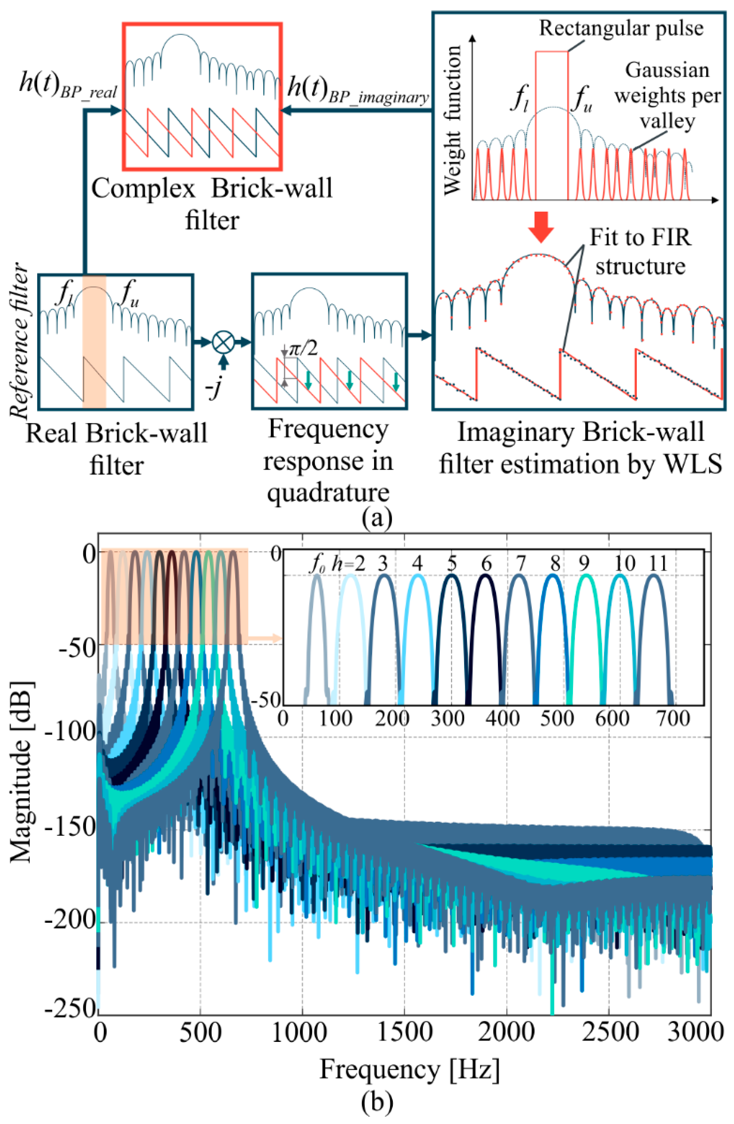
The proposed methodology for phasor estimation is depicted in Figure 1. The first stage consists of the estimation of both the fundamental component phasor and its frequency, where the amplitude and phase are computed by means of the analytic signal (x(t)_r + ix(t)_i [27]) obtained through the proposed complex FIR filter. This filter is designed from the frequency response of a reference band-pass filter as shown in Figure 2a. The reference filter given by Equation (6) represents the real filter, h(t)_r. Then, from the real filter frequency response, a phase shift of π/2 is introduced by multiplying the real filter frequency response by −j in order to have the frequency response in quadrature. From this response, the weighted least square (WLS) algorithm is used to obtain the coefficients of the imaginary FIR filter by means of a fitting stage for the shifted frequency response. In order to improve the fit in the passband, a weight function for the fit based on both a rectangular pulse in the passband and a set of small Gaussian functions in the valleys of the frequency response are proposed, obtaining the imaginary filter (a filter in quadrature with the real filter). As a result, two brick-wall band-pass FIR filters (real: h(t)_{BP_real} and imaginary: h(t)_{BP_imaginary}) are obtained. These proposed steps to design the filter are needed since the filter performance has to satisfy the IEEE Std. C37.118.1 requirements.

For the estimation of the fundamental phasor, a brick-wall filter with a passband of 53 Hz to 67 Hz with a filter order of 1024 (similar to the filter of 10 cycles presented at the Std.) is carefully selected to obtain an attenuation greater than 50 dB for frequencies out of the Nyquist frequency given by the reporting rate in frames per second (FPS)/2. In the same way, complex brick-wall FIR filters for harmonic components with both a passband of ±15 Hz around the nominal harmonic component and a filter order of 768 are designed. The amplitude frequency responses for the proposed filter bank are shown in Figure 2b. As can be notice, a lower order is proposed for the harmonic filters in order to reduce the latency since the next stage, i.e., the SSB modulation, also produces a latency.

From the outputs of the complex filter, x(t)_r and x(t)_i, the instantaneous amplitude can be easily estimated by:

$$A=\frac{1}{\sqrt{2}}\sqrt{x{(t)}_r^2+x{(t)}_i^2}$$

(8)

where x(t)_r and x(t)_i, are the in-phase and in-quadrature filtered signals. Additionally, a magnitude compensation is carried out when a frequency deviation occurs. This compensation is necessary due to the magnitude frequency response of the filter. In order to reduce the computational burden, a simple Gaussian function Gc is proposed for the compensation process. Hence, the compensated magnitude A(t)c is given by:

$$A{(t)}_c=\frac{A(t)}{Gc}=\frac{A(t)}{e^{-{\left(\frac{f(t)-f_0}{\delta }\right)}^2}}$$

(9)

where f is the instantaneous frequency and δ is a shape parameter of the Gaussian function, which is adjusted according to the magnitude filter attenuation response, using a curve fitting technique in the interest range, this is ±5 Hz around f₀.

On the other hand, the instantaneous phase can be obtained as:

$$\theta (t)={\tan }^{-1}\left(\frac{x{(t)}_i}{x{(t)}_r}\right)$$

(10)

However, the instantaneous phase represents the entire argument of the sinusoidal signal shown in Equation (1), this means that the instantaneous phase is in a rotatory reference frame given by the nominal frequency 2πf₀t. Therefore, a phase compensation is presented to obtain an adequate phasor representation. It is given by:

$$\theta {(t)}_{stat}=\theta (t)-2\pi f_{0}t$$

(11)

where θ(t)_stat is the phase in a stationary reference frame. This phase value contains the instantaneous frequency deviation term along with the stationary phase. The instantaneous phase is used as argument for the SSB modulation depicted in Figure 3a. A Hilbert FIR filter with a π/2 phase using an equirriple linear-phase and an order of 600 is proposed to obtain the analytic signal terms, i.e., x(t) and $\widehat{x}$(t). Then, these terms are modulated by a cosine and sine functions (see Figure 3a), respectively, using the inverted instantaneous phase and the harmonic order h; as a result, the frequency shift depicted in Figure 3b is achieved. From this point of view, it is evident that a unit of SSB modulation is required for each harmonic component (see Figure 1). Additionally, it should be pointed out that Equation (5) has to be modified in order to consider the frequency deviation as a time-variant frequency signal; therefore, the instantaneous SSB modulation is computed by:

$$x{(t)}_{SSB}=x(t)\cos (-2\pi h{\displaystyle \int \Delta fdt}-{\varphi }_h)-\widehat{x}(t)\sin (-2\pi h{\displaystyle \int \Delta fdt}-{\varphi }_h)$$

(12)

After that, the harmonic phasor estimation is computed by means of a bank of complex band-pass FIR filters, where the magnitude and phase are estimated using Equations (8) and (10). It is important to note that the magnitude compensation is not required for the harmonic components since the SSB modulation centers all the harmonics to each filter, resulting in a 0 dB gain. Nevertheless, harmonic phase estimation does requires both a compensation due to the modulation process and a change of phase reference frame, which is summarized by the following equation (see also Figure 1):

$$\theta {(t)}_{stat\_h}=\theta {(t)}_h-h\theta {(t)}_{stat}-2\pi h{f}_{0}t$$

(13)

where θ(t)_h is the instantaneous phase of h-th harmonic, the term hθ(t)_s is the phase introduced by the SSB modulation by considering the harmonic order, and 2πhf₀t is the term due to the rotatory reference frame.

For the fundamental frequency estimation (see Figure 1), a derivative process that considers the instantaneous phase component (initial phase and frequency deviation) is used as follows:

$$f(t)=f_0+\frac{1}{2\pi }\frac{d\theta {(t)}_{stat}}{dt}$$

(14)

In the same way, the instantaneous frequency for harmonic components is obtained by means of the fundamental frequency as follows:

$$f{(t)}_h=hf(t)$$

(15)

The derivative process is based on the proposed algorithm in the IEEE Std. C37.118.1-2011 which is composed by a discrete differential equation [10]. In this regard, the derivative algorithm can be structured into a FIR filter architecture, simplifying its implementation. This filter has the following coefficients b_k= {12, −6, −4, −2}/(20/Fs) and can be implemented using a well-known FIR filter structure as follows:

$$y[n]={\displaystyle \sum _{k=0}^K{b}_{k}x[n-k]}$$

(16)

where x[n] is the discrete input signal, y[n] is the output signal and K is the filter order. As can be noticed in Figure 1, additional low-pass FIR filters are proposed to smooth the instantaneous phase of the fundamental component, which allows improving the accuracy in the SSB modulation process. Likewise, harmonic frequency components are filtered by a low-pass FIR filter to smooth the derivative process and improve the frequency accuracy. These filters are proposed as triangular filters with an order of 128. This order is selected by trial and error according to its performance and by considering the general delay time. A triangular weighted FIR filter is given by:

$$W(k)=1-\frac{2}{N+2}\left|k\right|$$

(17)

where k = −N/2:N/2 (integers only) and N is the filter order [10]. Finally, a downsampling process is carried out for the magnitude, phase, and frequency components. This process represents the reporting rate or FPS of the PMU. In this work, a 60 fps is used to assess the proposed algorithm.

4. Results and Discussions

The proposed algorithm is tested using all the benchmark tests proposed by the current synchrophasor IEEE standards: C37.118.1-2011 along with C37.118.1a-2014. All the experimentation is carried out using MATLAB software (The MathWorks, Inc., Natick, MA, USA). Steady-state and dynamic tests are carried to evaluate the accuracy through error parameters such as: TVE, FE, and RFE. As mentioned above, the error limits are extended to harmonic components in the most tests except in the modulation tests where the error boundaries depend on the carrier frequency and some adjustments must be carried out. Additionally, the dynamic behavior is also evaluated using parameters such as response time and delay time along with the overshoot by means of the step response. As the PMU standard is designed for a fundamental synchrophasor, additional issues must be considered, e.g., the signal sampling frequency Fs is set to 6000 Hz which allows analyzing up to 50th harmonic. This condition is also useful for the out-of-band interference test.

For the tests, a synthetic reference signal with 11 harmonic components is proposed, including even and odd harmonics. This number has been chosen by other authors; however, other harmonic phasors can be computed in the proposal by simply adding the corresponding stages (e.g., the SSB stage for a specific harmonic). The magnitude, phase, and frequency parameters of the synthetic signal are listed in

Table 1. Harmonic parameters for synthetic signals and estimated parameters by the proposed algorithm.

h	Proposed Parameters			Estimated Parameters
	Ah [p.u.]	ϕh [rad]	hfc [Hz]	Ah [p.u.]	ϕh [rad]	hfc [Hz]
1	1.000	0.0	60.000	1.000	−6 × 10−11	60.000
2	0.493	0.0	120.000	0.493	2 × 10−4	120.000
3	0.510	0.0	180.000	0.510	5 × 10−5	180.000
4	0.188	0.0	240.000	0.188	−8 × 10−4	240.000
5	0.375	0.0	300.000	0.375	−1 × 10−4	300.000
6	0.104	0.0	360.000	0.104	−3 × 10−4	360.000
7	0.208	0.0	420.000	0.208	1 × 10−4	420.000
8	0.101	0.0	480.000	0.101	3 × 10−4	480.000
9	0.202	0.0	540.000	0.202	3 × 10−4	540.000
10	0.100	0.0	600.000	0.100	−2 × 10−4	600.000
11	0.200	0.0	660.000	0.200	4 × 10−6	660.000

. This table also shows the estimated parameters using the proposal, where very similar values are obtained, indicating a suitable performance. These parameters are obtained in both steady-state and nominal conditions.

After that, the proposal is tested under all the benchmark tests according to the Std. C37.118.1-2011 and C37.118.1a-2014 using TVE, FE, and RFE. These tests include steady-state conditions (a specific parameter changes in a moment of time and then maintains its value) and dynamic conditions (a specific parameter changes overtime).

The TVE is a value which encompasses magnitude and phase accuracy. It is defined as:

$$\mathrm{TVE}=\sqrt{\frac{{(x_r^{\prime }-x_r)}^2+{(x_i^{\prime }-x_i)}^2}{x_r{}^2+x_i{}^2}}$$

(18)

where x′_r and x′_i are the estimated values, while x_r and x_i are the theoretical values given by the synthetic signal. Likewise, frequency and ROCOF measurements are evaluated by means of FE and RFE defined by:

$$\mathrm{FE}=\left|f-f^{\prime }\right|$$

(19)

$$\mathrm{RFE}=\left|(df/dt)-(d{f}^{\prime }/dt)\right|$$

(20)

where f and df/dt are the measured values and f′ and df′/dt are the true values at the same instant of time. In this work, ROCOF is obtained as the difference between the current values and the past values by dividing the result by Fs.

4.1. Steady-State Tests

4.1.1. Magnitude and Phase Tests

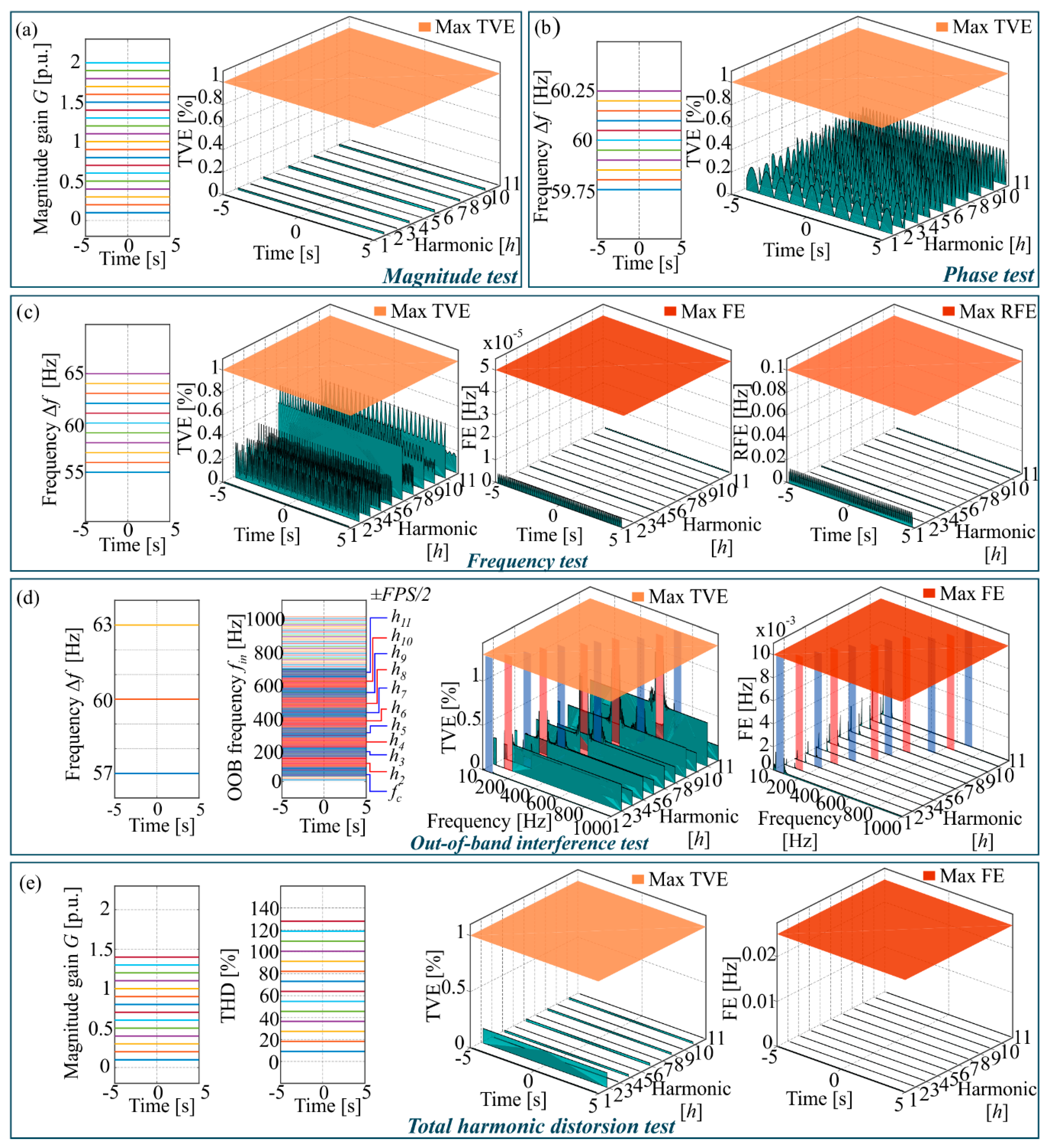
This test consists of evaluating the synchrophasor algorithm under constant changes of magnitude and phase. For the magnitude test, values between 0.1 p.u. to 2 p.u. (per unit) have to be tested [10]. Therefore, the signal under analysis with harmonic content is given by:

$$x(t)=G{\displaystyle \sum _{h=1}^H{A}_h\cos (h(2\pi f_{0}t+2\pi {\displaystyle \int \Delta fdt)}+{\varphi }_h)}$$

(21)

where G is a gain term that scales the entire signal between 0.1 and 2 as shown in Figure 4a. The TVE values for each harmonic component are also shown. A shaded plane is placed on the TVE graph, denoting the maximum allowable limit by the standard, i.e., 1%. As can be noticed, the TVE values for all harmonics remain far below the TVE boundaries.

For the phase test, the change of phase angle is carried out as described in [10] with an input frequency offset |Δf − f₀| < 0.25 Hz, which produces a slowly varying phase angle of ±π. The TVE values for the phase test are below the required limits (see Figure 4b), but an increment in the TVE values according to the harmonic order is observed. This effect is caused because the frequency deviation increases linearly according to the harmonic order.

4.1.2. Frequency Test

This test considers off-nominal frequency values, i.e., Δf = ±5 Hz. The main advantage of the proposed methodology is that the SSB modulation centers the harmonic frequencies in their respective passbands according to the fundamental frequency deviation, allowing an accurate result during the harmonic phasor estimation. TVE, FE, and RFE values are within the admissible levels of the IEEE Std. C37.118.1-2011 and C37.118.1a-2014 as shown in Figure 4c. Although allowable error levels are obtained, it can be noticed that even harmonic components have greater TVE errors than the ones obtained for the odd harmonic components, which is due to changes in the frequency response of the filters.

4.1.3. Out-of-Band (OOB) Interference Test

In this test, the inter-harmonic immunity is evaluated, where frequency deviations of Δf = ±0.1(FPS/2) = ±3 Hz are considered. The OOB interference is constructed by adding to the reference signal a set of sinusoidal components with 10% of fundamental magnitude from 10 Hz to 1000 Hz, which represents a greater range (a more realistic condition for harmonics) than the one required by the standard. Hence, the reference signal for this test is:

$$x(t)={\displaystyle \sum _{h=1}^H{A}_h\cos (2\pi h(f_{0}t+{\displaystyle \int \Delta fdt)}+{\varphi }_h)}+0.1\sin (2\pi f_{in}t)$$

(22)

where f_in is the OOB interference frequency. The reported TVE and FE values exclude the Nyquist frequency of the synchrophasor reporting rate, i.e., ±FPS/2 around each component as shown in Figure 4d (blue and red zones). The TVE and FE values are below the limits required by the synchrophasor standard. For the TVE values, high values or peaks close to the Nyquist frequency can be observed but they remain within the required accuracy. It is important to mention that although a frequency deviation along with the OOB interference are evaluated, the SSB modulation and the high rejection of the proposed filters (below 50 dB beyond the Nyquist frequency) allow keeping the required accuracy, knowing that this test is one of the most demanding tests.

4.1.4. Total Harmonic Distortion (THD) Test

For this test, the standard requirements set a 10% of THD. In order to have a wider range of evaluation and by considering the presence of even and odd harmonics, higher values of THD are considered. In the proposed evaluation, the THD variation is proposed by scaling all the harmonic components of the reference signal as follows:

$$x(t)=A_1\cos (2\pi f_{0}t+2\pi {\displaystyle \int \Delta fdt}+{\varphi }_1)+G{\displaystyle \sum _{h=2}^H{A}_h\cos (h(2\pi f_{0}t+2\pi {\displaystyle \int \Delta fdt)}+{\varphi }_h)}$$

(23)

where G is a constant gain that changes from 0.1 to 1.4, producing THD values from 10% to 130% approximately as shown in Figure 4e; as can be noticed, the accuracy of the synchrophasor and frequency is not affected by high levels of THD. Although the limits are not exceeded, even harmonic components have greater error values than the ones obtained for the odd harmonic components, which is similar to the frequency test (Figure 4c).

4.2. Dynamic Tests

4.2.1. Magnitude and Phase Modulation Tests

In this test, bandwidth requirements for synchrophasors are evaluated by means of magnitude or phase modulated signals. These signals are obtained as follows:

$$x(t)={\displaystyle \sum _{h=1}^H\left(A_h(1+k_x\cos (2\pi f_m))\cos (2\pi h{f}_{0}t+k_{a}h\cos (2\pi f_m-\pi )\right)}$$

(24)

where k_x is the amplitude modulation factor, k_a is the phase modulation factor, and f_m is the modulation frequency. The magnitude modulation test is performed using k_x = 0.1 and k_a = 0, and the phase modulation test is performed with k_x = 0 and k_a = 0.1 as described in the standard. In both cases, the modulation frequency varies from 0.1 Hz to 5 Hz in steps of 0.2 Hz.

Regarding the magnitude modulation test (see Figure 5a), TVE values below 3% are obtained, staying within the allowable ranges. The results for the fundamental component have levels of accuracy close to the maximum TVE limit; however, the FE and RFE values have good performance.

For the phase modulation test, the TVE performance is similar to the one obtained in the magnitude modulation, which is below the maximum allowable TVE value, i.e., 3%. Regarding the frequency and ROCOF results for the phase test, some issues must be considered since the maxima allowable FE and RFE values depend on the modulation frequency values which increase according to the harmonic order. In this regard, as described in the C37.118.1a-2014, the maxima allowable FE and RFE values for harmonic components are set by:

$$\mathrm{Max}\mathrm{FE}=0.06h{f}_m$$

(25)

$$\mathrm{Max}\mathrm{RFE}=0.18\pi h{f}_m{}^2$$

(26)

As shown in Figure 5b, the FE and RFE maxima values are indicated by means of shaded inclined planes where the measurements show values below the boundaries.

4.2.2. Frequency Ramp Test

Dynamic performance during a frequency change is tested with a linear frequency ramp which is constructed using the following equation:

$$x(t)={\displaystyle \sum _{h=2}^H{A}_h\cos (2\pi h{f}_{0}t+\pi h{R}_f{t}^2})$$

(27)

where R_f is the frequency ramp rate in Hz/s and the frequency range is given by the test duration. The most demanding condition for this test ranges between ±5 Hz. Then, positive and negative frequency ramps are constructed. As shown in Figure 5c, a positive ramp test is carried out from 55 Hz to 65 Hz where TVE, FE, and RFE values are evaluated according to the class M performance. As can be observed, the magnitude, phase, frequency, and ROCOF measurements have the enough accuracy for synchrophasor applications. Likewise, a negative slope ramp is also tested as shown in Figure 5d. In this test, similar error values are obtained, complying with the accuracy requirements for phasor, frequency, and ROCOF.

4.2.3. Magnitude and Phase Step Tests

Step tests are carried out to assess the time performance of synchrophasor, frequency, and ROCOF measurements using parameters such as response time, delay time, and overshoot, whose limits depend on the FPS value. The main idea is to produce a step of 10% in the magnitude test and a step of π/18 in the phase for the phase step. For the measurements of time and overshoot, a set of shifted steps in a constant fraction of the reported interval are used to interleave them, obtaining higher resolutions [10]. The delay time is obtained by measuring the time interval between the zero time of the step input and the 50% of the final value, while the response time is measured by means of the TVE as the time interval that begins when the TVE exceeds the allowable limit and ends when it returns and remains below the limit [10]. Similar to the TVE value, the frequency and ROCOF time responses are measured using the FE and RFE values. Regarding the overshoot, it is measured as a percentage between the maximum value and the final value. A more detailed description of the aforementioned parameters can be found in [10].

The results for the magnitude and phase tests are summarized in

Table 2. Magnitude and phase tests results for each harmonic component.

	Magnitude Step Test					Phase Step Test
h	Response Time (Max. 7/FPS)	Delay Time (Max. 1/(4FPS))	Overshoot (Max. 10%)	Frequency Response Time (Max. 14/f0)	ROCOF Response Time (Max. 14/f0)	Response Time (Max. 7/FPS)	Delay Time (Max. 1/(4FPS))	Overshoot (Max. 10%)	Frequency Response Time (Max. 14/f0)	ROCOF Response Time (Max. 14/f0)
1	0.0594 s	0.00018 s	0.022%	0.0874 s	0.0190 s	0.06960 s	0.0001000 s	0.00%	0.1292 s	0.1456 s
2	0.0342 s	0.00018 s	0.550%	0.1189 s	0.1035 s	0.06940 s	0.0000520 s	6.26%	0.1383 s	0.1546 s
3	0.0340 s	0.00022 s	0.290%	0.1212 s	0.1328 s	0.09420 s	0.0000590 s	4.55%	0.1396 s	0.1563 s
4	0.0385 s	0.00027 s	0.950%	0.1219 s	0.1374 s	0.10000 s	0.0000120 s	* 11.25%	0.1401 s	0.1572 s
5	0.0342 s	0.00033 s	0.260%	0.1225 s	0.1382 s	0.09920 s	0.0000560 s	4.39%	0.1411 s	0.158 s
6	0.0448 s	0.00044 s	1.140%	0.1265 s	0.1386 s	0.10140 s	0.0000006 s	* 14.21%	0.1416 s	0.1584 s
7	0.0350 s	0.00051 s	0.270%	0.1347 s	0.1390 s	0.10090 s	0.0000270 s	5.41%	0.1535 s	0.1586 s
8	0.0362 s	0.00062 s	0.680%	0.1408 s	0.1430 s	0.10220 s	0.0000007 s	* 11.82%	0.1688 s	0.1589 s
9	0.0348 s	0.00068 s	0.250%	0.1408 s	0.1517 s	0.10240 s	0.0000550 s	4.43%	0.1714 s	0.1591 s
10	0.0359 s	0.00074 s	0.630%	0.1412 s	0.1561 s	0.10370 s	0.0000021 s	8.59%	0.1734 s	0.1592 s
11	0.0351 s	0.00077 s	0.260%	0.1416 s	0.1574 s	0.10400 s	0.0000650 s	4.16%	0.1746 s	0.1594 s

* Values that exceed the allowable limits.

, where the step test is applied to each harmonic by considering a 10% of magnitude and π/18 rad of phase step. In the magnitude step tests, the maximum response time is 0.0594 s for the fundamental component which is below the allowed value for 60 FPS (0.116 s). The maximum delay time is 0.00077 s measured for the 11th harmonic component, it is also below the allowable limit (0.004166 s); besides that, overshoot values below 1.140% are obtained for the magnitude step tests. In the cases of frequency and ROCOF response times, the maxima times are measured in the 11th harmonic component, 0.1416 s and 0.1574 s, respectively. For the phase tests, the maximum response time is achieved by the 11th harmonic component (0.10400 s) which is close to the maximum allowable limit. Delay time in the phase step test shows a behavior within the limits with a maximum delay time of 0.0001 s, which is obtained for the fundamental component. In the overshoot measurements for the phase step tests, some drawbacks can be observed since the 4th, 6th, and 8th harmonic components exceed the overshoot percentage with values of 11.25%, 14.21%, and 11.82%, respectively. Nevertheless, these drawbacks are present only for even components while odd components have values below 5.41%. Requirements for frequency and ROCOF time responses are completely accomplished with maxima values of 0.1746 s and 0.1594 s, respectively, obtained for the 11th harmonic component. Finally, although an increment in the response time for frequency and ROCOF values can be noticed for the magnitude and phase step tests according to the harmonic order, the limits are not exceeded; in fact, they are far below the allowed limits, hence, the number of harmonics to be measured can be extended.

4.3. Comparison with Previous Works

As aforementioned some strategies have been reported for phasor harmonic estimation with PMU capabilities, which are summarized in

Table 3. Comparative summary between the proposed method and other related works.

Work	Methodology	Additional Frequency Tracking	Static Test Validation	Dynamic Test Validation	Harmonics under Test	PMU Reporting Frequency (FPS)	Reported Error Values
[2]	1. Signal decimation. 2. Apply window to signal. 3. Apply FFT for synchrophasor estimation. 4. Compensation for off-nominal frequencies	Yes	Yes	No	3, 5, 7, and 9	10	1. TVE2. Standard deviation
[9]	1. Adaptive filter bank (FIR, Kalman and SFFT) for each harmonic component. 2. Phasor estimation.	Yes	Yes	Yes	2, 3, 4, 5, 6, 7, 8, 9, 10, 11	60	1. Magnitude Error. 2. Frequency error. 3. THD error
[12]	1. Apply window to signal.2. Apply FFT for synchrophasor estimation.	Yes	Yes	No	3, 5, 7, 9	10	-
[19]	1. Vector state model estimation. 2. Frequency tracking for compensation. 3. Harmonic phasor estimation	Yes	Yes	Yes	3, 5	-	1. TVE
This work	1. Fundamental phasor and frequency estimation through a complex filter. 2. Instantaneous SSB modulation to center the harmonic component. 3. Harmonic phasor estimation.	No	Yes	Yes	2, 3, 4, 5, 6, 7, 8, 9, 10, 11	60	1. TVE 2. FE 3. RFE 4. Response time 5. Delay time 6. Overshoot

- Not reported values.

. These strategies are based on FFT [2,12], adaptive filters [9], and model-based estimation [19]. It is important to mention that the current methods require additional frequency tracking algorithms for an accurate estimation when off-nominal frequencies are present, unlike the proposed work where the frequency is estimated by means of the proposed algorithm. On the other hand, different tests must be carried out to evaluate the robustness under different static and dynamic conditions that can occur in real scenarios; however, not all works consider the different possible conditions, such as in [2,12]. Regarding the harmonic estimation, different harmonic orders and reporting rates are analyzed; nevertheless, odd and even harmonics are only considered in [9] and the proposed work. Although the proposal only analyzes up to the 11th harmonic, the computation of a higher number of harmonics requires simply to add the stages related to the harmonic components as shown in Figure 1. In fact, the proposal can be configured to compute specific harmonic phasors according to the user application, e.g., protection and control schemes for some odd harmonics. Finally, although there is no guidelines for harmonic phasor estimation oriented to PMU applications, different error criteria are used to assess the performance of the proposed methodologies, where the proposed work uses all the benchmark tests and accuracy requirements indicated in the current synchrophasor standard.

5. Conclusions

A new algorithm for phasor and frequency estimation of fundamental and harmonic components is assessed through the current synchrophasor standards, i.e., the Std. C37.118.1-2011 along with Std. C37.118.1a-2014. The proposed algorithm is based on complex brick-wall FIR filters which are designed at the nominal frequencies for fundamental and harmonic components, while the instantaneous SSB modulation technique is used to shift the harmonic frequency component according to the instantaneous frequency deviation, shifting the signal to the center of each complex FIR filter.

The proposed filters show that are reliable enough to accomplish with the PMU standards due to their high rejection in the stop band, linear phase behavior, and fast response time. Additionally, the main advantage of the proposal is that additional algorithms for frequency tracking are not required as the case of the most harmonic phasor estimation algorithms reported in the literature, which implies a complexity reduction. It is worth noting that even and odd harmonic components are considered in the analysis, which is not always studied in the works proposed for the harmonic phasor estimation.

The fulfillment of all the dynamic and steady-state tests stated in the PMU standard is achieved, taking as a reference the limits for the fundamental phasor; yet, some issues must be considered. Firstly, in the phase modulation test, the maxima allowable limits are modified according to the harmonic order since the phase modulation affects the frequency components related to the allowed maximum error. Secondly, although some overshoot values are out of range in the phase step tests for some even harmonic components, the time performance still has admissible results and they do not affect the estimation accuracy. Finally, the proposed algorithm is tested for eleven components but it could be extended for more harmonic components easily.

In a future work, the proposal will be implemented using the FPGA technology, exploiting its parallelism. This implementation will allow providing a system-on-a-chip (SoC) solution for PMU applications in power systems.