Fast Imaging of Short Perfectly Conducting Cracks in Limited-Aperture Inverse Scattering Problem


Department of Information Security, Cryptography, and Mathematics, Kookmin University, Seoul 02707, Korea
Electronics 2019, 8(9), 1050; https://doi.org/10.3390/electronics8091050
Submission received: 4 September 2019
/
Revised: 11 September 2019
/
Accepted: 15 September 2019
/
Published: 18 September 2019
(This article belongs to the Special Issue Microwave Imaging and Its Application)
Abstract
:In this paper, we consider the application and analysis of subspace migration technique for a fast imaging of a set of perfectly conducting cracks with small length in two-dimensional limited-aperture inverse scattering problem. In particular, an imaging function of subspace migration with asymmetric multistatic response matrix is designed, and its new mathematical structure is constructed in terms of an infinite series of Bessel functions and the range of incident and observation directions. This is based on the structure of left and right singular vectors linked to the nonzero singular values of MSR matrix and asymptotic expansion formula due to the existence of cracks. Investigated structure of imaging function indicates that imaging performance of subspace migration is highly related to the range of incident and observation directions. The simulation results with synthetic data polluted by random noise are exhibited to support investigated structure.
1. Introduction
This paper concerns the application of so-called subspace migration to determine the location of a set of small cracks from measured far-field data in limited-aperture problem. The general framework of subspace migration for determining perfectly conducting cracks was presented in the work by the authors of [1]. This framework was based on the asymptotic expansion formula in the presence of the crack and the structure of singular vectors of multistatic response (MSR) matrix under the assumption of coincident transmitter and receiver arrays. Throughout several extensions [2,3,4,5], it turned out that subspace migration is fast, stable, and effective noniterative technique for identifying arbitrary shaped inhomogeneities in both full- and limited-view inverse scattering problems.
Unfortunately, throughout several real-world applications, such as biomedical imaging [6], synthetic aperture radar (SAR) [7], ground-penetrating radar (GPR) [8], photoacoustic tomography [9], the detection of inhomogeneities buried in the ground [10], physical optics [11], and crack detection of concrete void [12], the assumption of coincident transmitter and receiver arrays is not valid. This means that the MSR matrix is no longer symmetric so that it is impossible to apply traditional subspace migration. This gives a stimulus for this study to design subspace migration in limited-aperture inverse scattering problem.
The main purposes of this contribution are designing an imaging function for imaging of a set of perfectly conducting cracks with small length in two-dimensional limited-aperture inverse scattering problem and exploring the mathematical structure of imaging function by constructing a relationship with an infinite series of Bessel functions of integer order and the range of incident and observation directions. This is based on the structures of the left and right singular vectors of the asymmetric MSR matrix and the asymptotic expansion formula due to the presence of such cracks. From the explored structure, we can examine that the imaging performance is significantly dependent on the range of incident and observation directions.
This contribution is organized as follows. In Section 2, we briefly introduce the two-dimensional direct scattering problem and far-field pattern in the presence of a set of perfectly conducting cracks with small length. Section 3 contains an introduction on the subspace migration and analysis on the structure of imaging function in the limited-aperture inverse scattering problem. In Section 4, we present several numerical experiments with synthetic data polluted by the random noise to support analyzed structure, and Section 5 presents a short conclusion.
2. Direct Scattering Problem and Far-Field Pattern
We introduce the two-dimensional direct scattering problem due to presence of S different well-separated perfectly conducting cracks, denoted by , with length , . For a more detailed description, see the works by the authors of [13,14,15]. Throughout this paper, we assume that is represented as follows,
for . Here, denotes the rotation by and we denote be the center of . We let be the collection of all and k be the fixed positive wavenumber, which is of the form . Here, is given wavelength satisfies for all s.
In this paper, we consider the plane-wave illumination: we let be the given incident field with propagation direction , where denotes the two-dimensional unit circle centered at the origin. Let us denote be the time-harmonic total field which satisfies the Helmholtz equation: for ,
with the Dirichlet boundary condition
Let be the scattered field which satisfies the Sommerfeld radiation condition
uniformly in all the directions . The far-field pattern of scattered field is given by the following relation,
uniformly in all the directions . Based on [15], can be represented as the single-layer potential with unknown density function :
3. Single-Frequency Subspace Migration in Limited-Aperture Problem: Introduction, Analysis, and Numerical Simulations
3.1. Introduction to Imaging Function of Subspace Migration
In this section, the imaging function of the subspace migration for identifying locations of from a set of measured far-field patterns, such that
where and are set of observation and incident directions, respectively, refer to Figure 1, and and are given by
respectively. Throughout this paper, we assume that and are connected, proper subsets of and total number of observation and incident directions satisfy .
Note that as the exact formulation of of (3) is still unknown, we need an alternative expression of for introducing imaging function. Based on the work by the authors of [13], the far-field pattern can be represented as the following asymptotic expansion formula, which plays a key role in the introduction and analysis of the imaging function of the subspace migration.
Lemma 1
Now, let us introduce the imaging function of subspace migration. From the collection of far-field pattern data , let us generate the following multistatic response (MSR) matrix :
Then, the singular value decomposition (SVD) of can be written by
where the superscript ∗ represents the Hermitian operator, , , and . and are the left- and right-singular vectors of , respectively, and denotes singular value of , such that
From the (4), the elements of can be approximated as
This representation yields us to introduce unit test vectors: for ,
where, denotes the region of interest. Then, on the basis of the work by the authors of [1], we can observe the following relationships,
where . Based on above relations, we can introduce the following imaging function adopted by the subspace migration,
Then, we can easily check that the map of will contain peak of magnitude 1 at and small one at . Therefore, it will be possible to identify locations of all small cracks. The complete procedure used for imaging via subspace migration is summarized in Algorithm 1.
| Algorithm 1 Procedure of imaging via subspace migration at given wavenumber k. | |
| 1: procedure Subspace migration(k) | |
| 2: Initialize | |
| 3: for to M do | |
| 4: for to N do | |
| 5: collect far-field data | ▹ see (3) |
| 6: end for | |
| 7: end for | |
| 8: perform SVD of | ▹ see (5) |
| 9: select and | ▹ see (6) |
| 10: for do | |
| 11: evaluate and | ▹ see (7) |
| 12: initialize | |
| 13: for to S do | |
| 14: | |
| 15: end for | |
| 16: | |
| 17: end for | |
| 18: plot | |
| 19: end procedure | |
3.2. Analysis of Imaging Function
Although subspace migration is a promising noniterative technique for imaging unknown targets in limited-aperture inverse scattering problem, further mathematical theory to explain feasibilities, the effect on the range of incident and observation directions, and fundamental limitations. Here, we investigate mathematical expression of with an infinite series of Bessel functions of integer order and the range of incident and observation directions. The result follows.
Theorem 1
(Mathematical structure of imaging function). Let , , and . Then, for sufficiently large M and N, can be represented as follows
where denotes the Bessel function of integer order ν,
Proof.
As M and N are sufficiently large, the following relations hold uniformly (see [4,16] for instance); for and ,
where denotes the Bessel function of integer order . With this, by denoting , we can derive
where
Analogously, we can obtain
where
Finally, applying (8) again, we can obtain
This leads us to (10) and completes the proof. □
Remark 1
(Some properties of imaging function). On the basis of the result in Theorem (1), some properties of can be summarized as follows.
- 1.
- As and for all , we can examine that when for all s. This means that the terms and does not contribute to the imaging of cracks. Furthermore, due to the oscillating properties of Bessel functions, some artifacts will be appear in the map of .
- 2.
- The imaging performance of is significantly depending on the range of incident and observation directions. For a detail, if the range of incident or observations is narrow, i.e., if the value of either or is small, it will be very hard to recognize the location of because the term , which contributes to the imaging of cracks, is dominate by either or . Otherwise, if the range of both incident and observation directions is wide, it will be possible to obtain good results.
- 3.
- Based on the above observation, eliminating the terms and will be a method of improvement of imaging performance. Notice that since the secrackhing point is arbitrary, it is impossible to make . This means that one must find a condition to satisfyandOne possible selection is , i.e., full-aperture configuration. Another possible option is and . Unfortunately, this selection is ideal because we have no a priori information of the location of cracks. Nevertheless, this selection indicates us that if the range of both incident and observation directions is wider than π, it will be possible to obtain good result via the map of .
- 4.
- As the following asymptotic property holds for sufficiently large kit is possible to eliminate and by applying . However, this is an ideal condition.
- 5.
- In the limited-view problem, i.e., if for with then since , can be expressed asThis is the same result derived in the work by the authors of [17].
- 6.
- In the full-aperture problem, i.e., if then since , can be expressed asThis is the same result derived in [4].
4. Simulation Results
4.1. Imaging of Well-Separated Small Cracks
Some results of numerical simulation are exhibited here to support the theoretical result. For this, a set of three different cracks with the small length are chosen:
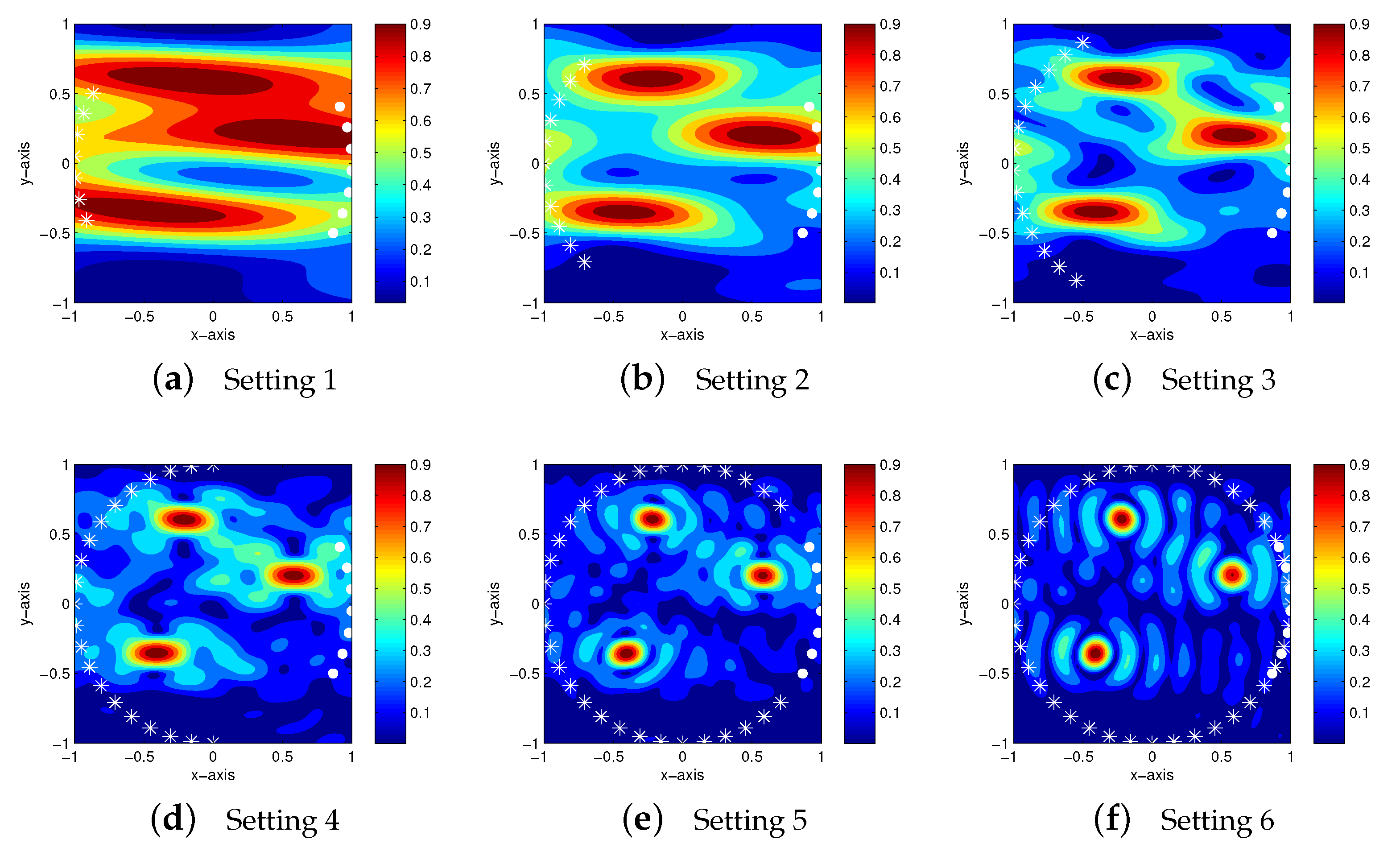
Thus, , , and . The ROI is set to , and the step size of is set to . The far-field elements of are obtained for by solving a Fredholm integral equation of the second kind along the cracks introduced in the work by the authors of [18]. The values of and M with are shown in Table 1. After the calculation of far-field pattern data, a 20 dB white Gaussian random noise is added to the unperturbed data.
Figure 2 shows maps of with , and . As we mentioned in (2) of Remark 1, the location of the cracks cannot be identified with Setting 1 (narrow range). Through the maps of with Setting 2 and 3, it is possible to recognize the existence of cracks but identification of their location is somehow difficult due to the appearance of blurring effect at the center of all , . In contrast, it is possible to identify the location of cracks with Settings 4, 5, and 6 and this supports the (3) of Remark 1.
4.2. Imaging of Closely Located Small Cracks: Resolution Limit
The purpose of numerical experiments in this section is to consider the resolution of the image. For this, a set of three different cracks with the small length are chosen:
Thus, , , and . Simulation configuration is same as the imaging of well-separated small cracks.
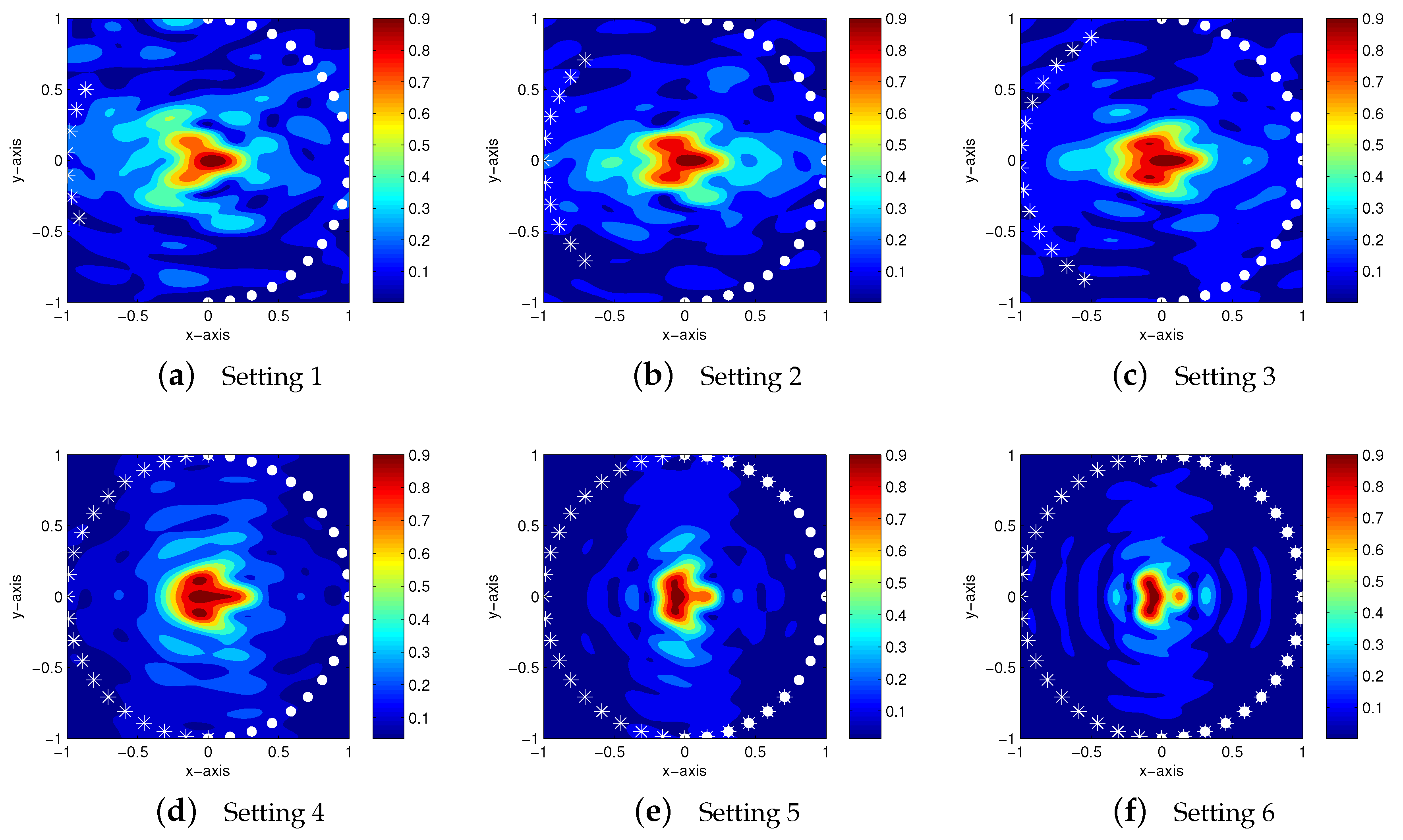
Figure 4 shows maps of with , and . This result clearly explains that throughout the imaging result with applied wavelength , it is impossible to distinguish three cracks. This result supports the Rayleigh resolution limit, refer to [19]. Figure 5 shows maps of with , and . Similarly, it is impossible to identify locations of three cracks even in the wide range of incident and observation directions.
4.3. Further Results: Imaging of Cracks with Neumann Boundary Condition
Here, we just exhibit imaging results of cracks with Neumann boundary condition. Same as the previous, we let be the given incident field with propagation direction and be the time-harmonic total field, which satisfies the Helmholtz equation
with the Neumann boundary condition
Here, denotes the unit outward normal vector at . In this case, the far-field pattern can be represented as the double-layer potential with unknown density function
Throughout several researches [4,20,21,22,23,24], estimation of at is essential to obtain good result. Unfortunately, we have no a priori information of crack, therefore an additional procedure for estimating is needed, but this requires large computational costs. Due to this, similarly to the imaging of crack with Dirichlet condition, we adopt the same imaging function (9),
Here, test vectors and are given in (7).
It is worth to mentioning that there is no asymptotic expansion formula for the far-field pattern because the density function of (12) is still unknown. Instead, on the basis of physical factorization of MSR matrix [20,25], we can derive the following outline mathematical expression of : Let , , , and . Then, for sufficiently large M and N,
where
A rigorous derivation of asymptotic expansion formula for the far-field pattern and mathematical structure of imaging function in the existence of perfectly conducting cracks with Neumann boundary condition will be an interesting and forthcoming research topic.
5. Conclusions
Based on the structure of the singular vectors of the MSR matrix, we designed an imaging function of subspace migration in limited-aperture inverse scattering problem. Throughout careful derivation, we investigated that the imaging function can be expressed by an infinite series of Bessel function of integer order and the range of incident and observation directions. On the basis of the theoretical result, various properties of imaging technique and least condition of incident and observation directions to guarantee a good result. The Simulation results with noisy data are exhibited to support the theoretical results and demonstrate the discovered properties. In this paper, the imaging of crack(s) with Dirichlet boundary condition was considered. Extension to the imaging of cracks with Neumann boundary condition will be considered in future work. Following several contributions [14,26,27,28,29], we found that the MUltiple SIgnal Classification (MUSIC) algorithm is an effective and stable noniterative imaging technique in inverse scattering problem. Investigation of mathematical structure of MUSIC-type imaging function in limited-aperture inverse scattering problem will be also an interesting research topic.
Funding
This research was supported by the Basic Science research Program through the National Research Foundation of Korea (NRF) funded by the Ministry of Education (No. NRF-2017R1D1A1A09000547).
Conflicts of Interest
The author declares no conflict of interest.
References
- Ammari, H.; Garnier, J.; Kang, H.; Park, W.K.; Sølna, K. Imaging schemes for perfectly conducting cracks. SIAM J. Appl. Math. 2011, 71, 68–91. [Google Scholar] [CrossRef]
- Ammari, H.; Garnier, J.; Kang, H.; Lim, M.; Sølna, K. Multistatic imaging of extended targets. SIAM J. Imag. Sci. 2012, 5, 564–600. [Google Scholar] [CrossRef]
- Borcea, L.; Papanicolaou, G.; Vasquez, F.G. Edge illumination and imaging of extended reflectors. SIAM J. Imag. Sci. 2008, 1, 75–114. [Google Scholar] [CrossRef]
- Park, W.K. Multi-frequency subspace migration for imaging of perfectly conducting, arc-like cracks in full- and limited-view inverse scattering problems. J. Comput. Phys. 2015, 283, 52–80. [Google Scholar] [CrossRef] [Green Version]
- Park, W.K. Real-time microwave imaging of unknown anomalies via scattering matrix. Mech. Syst. Signal Proc. 2019, 118, 658–674. [Google Scholar] [CrossRef]
- Acharya, R.; Wasserman, R.; Stevens, J.; Hinojosa, C. Biomedical imaging modalities: A tutorial. Comput. Med. Imaging Graph. 1995, 19, 3–25. [Google Scholar] [CrossRef]
- Kim, C.K.; Lee, J.S.; Chae, J.S.; Park, S.O. A modified stripmap SAR processing for vector velocity compensation using the cross-correlation estimation method. J. Electromagn. Eng. Sci. 2019, 19, 159–165. [Google Scholar] [CrossRef]
- Soldovieri, F.; Solimene, R. Ground penetrating radar subsurface imaging of buried objects. In Radar Technology; Kouemou, G., Ed.; IntechOpen: London, UK, 2010; Chapter 6; pp. 105–126. [Google Scholar]
- Cox, B.T.; Arridge, S.; Beard, P.C. Photoacoustic tomography with a limited-aperture planar sensor and a reverberant cavity. Inverse Probl. 2007, 23, S95–S112. [Google Scholar] [CrossRef]
- Delbary, F.; Erhard, K.; Kress, R.; Potthast, R.; Schulz, J. Inverse electromagnetic scattering in a two-layered medium with an application to mine detection. Inverse Probl. 2008, 24, 015002. [Google Scholar] [CrossRef]
- Mager, R.; Bleistein, N. An examination of the limited aperture problem of physical optics inverse scattering. IEEE Trans. Antennas Propag. 1978, 26, 695–699. [Google Scholar] [CrossRef]
- Taillet, E.; Lataste, J.F.; Rivard, P.; Denis, A. Non-destructive evaluation of cracks in massive concrete using normal dc resistivity logging. NDT E Int. 2014, 63, 11–20. [Google Scholar] [CrossRef]
- Ammari, H.; Kang, H.; Lee, H.; Park, W.K. Asymptotic imaging of perfectly conducting cracks. SIAM J. Sci. Comput. 2010, 32, 894–922. [Google Scholar] [CrossRef]
- Chen, X. Computational Methods for Electromagnetic Inverse Scattering; Wiley-IEEE: Hoboken, NJ, USA, 2018. [Google Scholar]
- Kress, R. Inverse scattering from an open arc. Math. Meth. Appl. Sci. 1995, 18, 267–293. [Google Scholar] [CrossRef]
- Ahn, C.Y.; Jeon, K.; Park, W.K. Analysis of MUSIC-type imaging functional for single, thin electromagnetic inhomogeneity in limited-view inverse scattering problem. J. Comput. Phys. 2015, 291, 198–217. [Google Scholar] [CrossRef]
- Kwon, Y.M.; Park, W.K. Analysis of subspace migration in limited-view inverse scattering problems. Appl. Math. Lett. 2013, 26, 1107–1113. [Google Scholar] [CrossRef]
- Nazarchuk, Z.T. Singular Integral Equations in Diffraction Theory; Mathematics and Applications Series; Karpenko Physicomechanical Institute, Ukrainian Academy of Sciences: Lviv, Ukraine, 1994. [Google Scholar]
- Ammari, H. An Introduction to Mathematics of Emerging Biomedical Imaging; Mathematics and Applications Series; Springer: Berlin, Germany, 2008; Volume 62. [Google Scholar]
- Hou, S.; Sølna, K.; Zhao, H. A direct imaging algorithm for extended targets. Inverse Problems 2006, 22, 1151–1178. [Google Scholar] [CrossRef]
- Park, W.K. Asymptotic properties of MUSIC-type imaging in two-dimensional inverse scattering from thin electromagnetic inclusions. SIAM J. Appl. Math. 2015, 75, 209–228. [Google Scholar] [CrossRef]
- Park, W.K. A novel study on subspace migration for imaging of a sound-hard arc. Comput. Math. Appl. 2017, 74, 3000–3007. [Google Scholar] [CrossRef]
- Park, W.K.; Lesselier, D. Electromagnetic MUSIC-type imaging of perfectly conducting, arc-like cracks at single frequency. J. Comput. Phys. 2009, 228, 8093–8111. [Google Scholar] [CrossRef]
- Park, W.K.; Lesselier, D. MUSIC-type imaging of a thin penetrable inclusion from its far-field multistatic response matrix. Inverse Probl. 2009, 25, 075002. [Google Scholar] [CrossRef]
- Hou, S.; Sølna, K.; Zhao, H. A direct imaging method using far-field data. Inverse Probl. 2007, 23, 1533–1546. [Google Scholar] [CrossRef] [Green Version]
- Ammari, H.; Iakovleva, E.; Lesselier, D. A MUSIC algorithm for locating small inclusions buried in a half-space from the scattering amplitude at a fixed frequency. Multiscale Model. Sim. 2005, 3, 597–628. [Google Scholar] [CrossRef]
- Ammari, H.; Kang, H. Reconstruction of Small Inhomogeneities from Boundary Measurements; Lecture Notes in Mathematics; Springer-Verlag: Berlin, Germany, 2004; Volume 1846. [Google Scholar]
- Marengo, E.A.; Gruber, F.K.; Simonetti, F. Time-reversal MUSIC imaging of extended targets. IEEE Trans. Image Process. 2007, 16, 1967–1984. [Google Scholar] [CrossRef] [PubMed]
- Zhong, Y.; Chen, X. MUSIC imaging and electromagnetic inverse scattering of multiple-scattering small anisotropic spheres. IEEE Trans. Antennas Propag. 2007, 55, 3542–3549. [Google Scholar] [CrossRef]
Figure 1.
Illustration of the set of incident directions , observation directions , and perfectly conducting crack .
Figure 1.
Illustration of the set of incident directions , observation directions , and perfectly conducting crack .
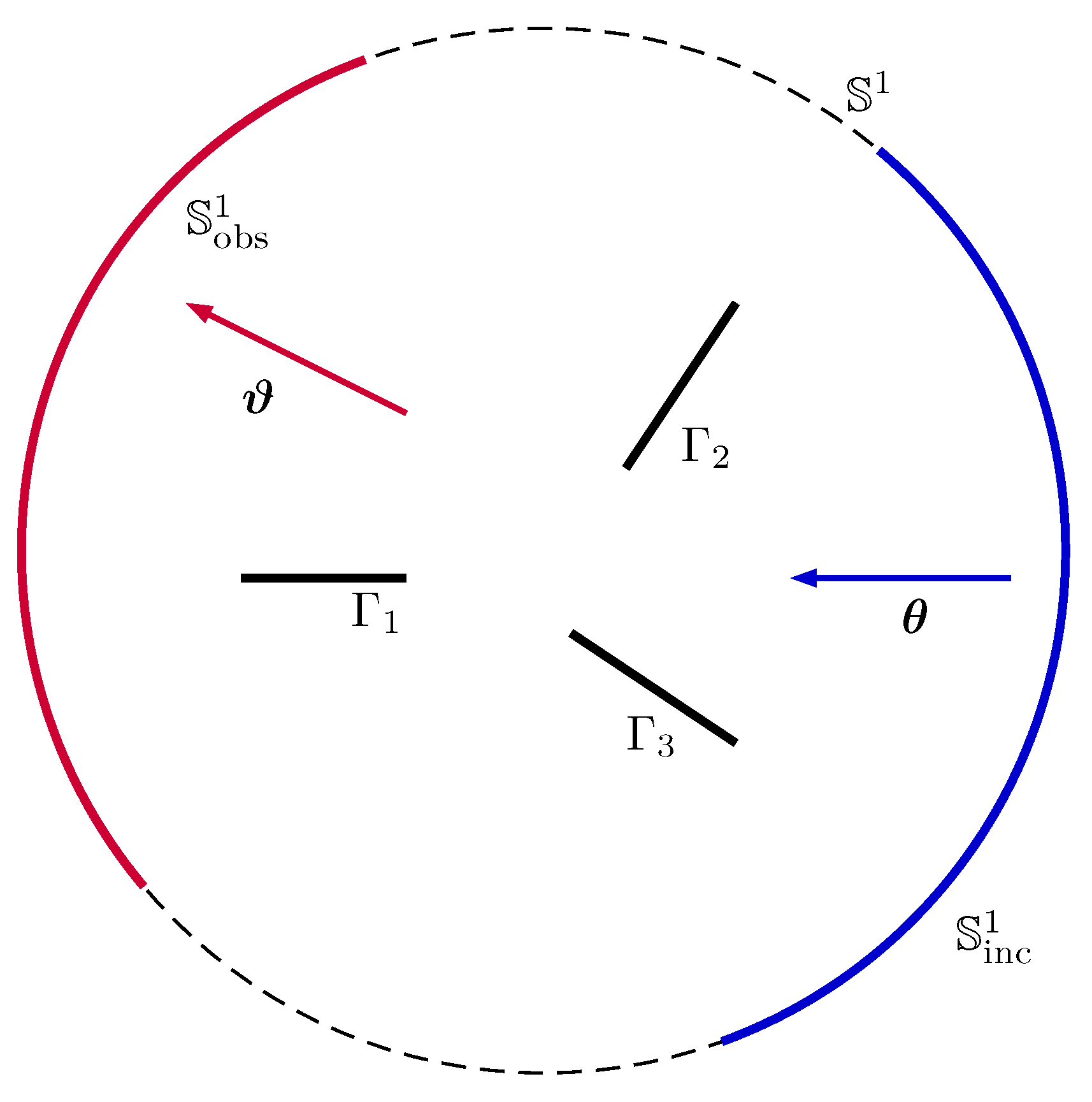
Figure 2.
Maps of . White colored marks o and 🟉 denote the incident and observation directions, respectively.
Figure 2.
Maps of . White colored marks o and 🟉 denote the incident and observation directions, respectively.

Figure 3.
Maps of . White colored marks o and 🟉 denote the incident and observation directions, respectively.
Figure 3.
Maps of . White colored marks o and 🟉 denote the incident and observation directions, respectively.
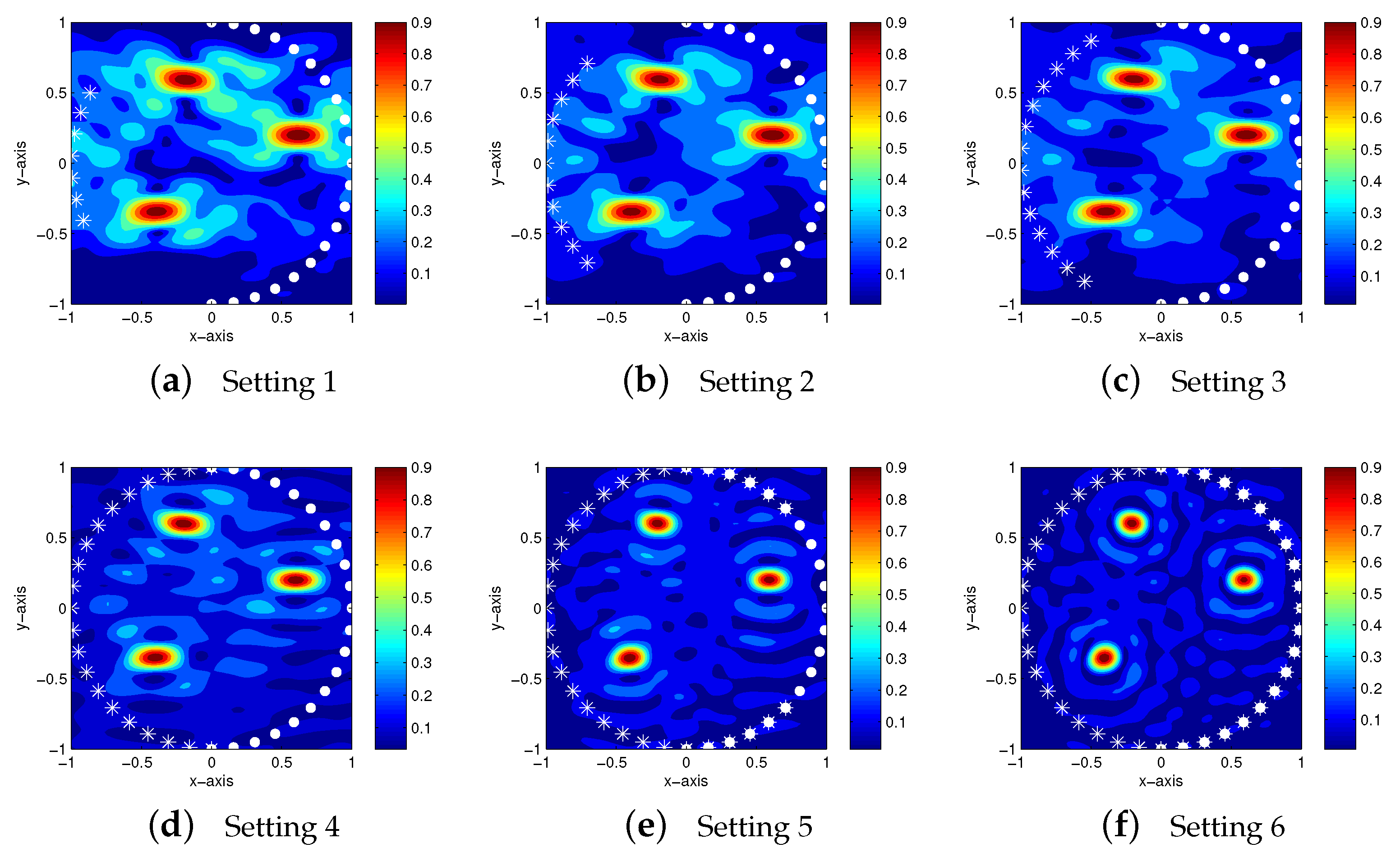
Figure 4.
Maps of . White colored marks o and 🟉 denote the incident and observation directions, respectively.
Figure 4.
Maps of . White colored marks o and 🟉 denote the incident and observation directions, respectively.
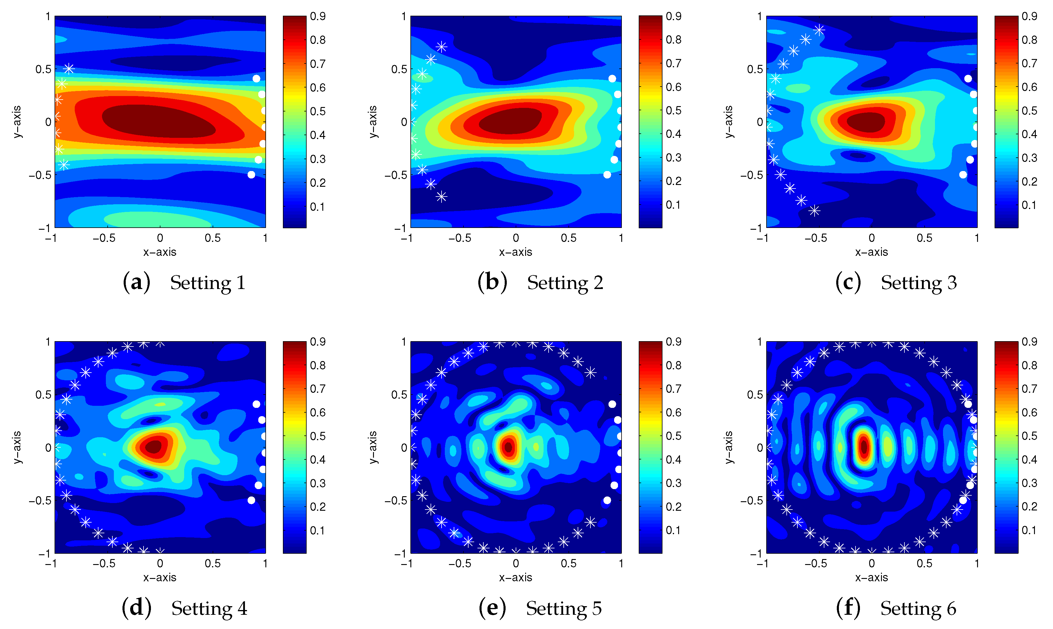
Figure 5.
Maps of . White colored marks o and 🟉 denote the incident and observation directions, respectively.
Figure 5.
Maps of . White colored marks o and 🟉 denote the incident and observation directions, respectively.

Table 1.
Test configuration for observation directions.
| Setting 1 | Setting 2 | Setting 3 | Setting 4 | Setting 5 | Setting 6 | |
|---|---|---|---|---|---|---|
| 0 | ||||||
| M | 7 | 11 | 14 | 21 | 31 | 41 |
© 2019 by the author. Licensee MDPI, Basel, Switzerland. This article is an open access article distributed under the terms and conditions of the Creative Commons Attribution (CC BY) license (http://creativecommons.org/licenses/by/4.0/).
Share and Cite
MDPI and ACS Style
Park, W.-K. Fast Imaging of Short Perfectly Conducting Cracks in Limited-Aperture Inverse Scattering Problem. Electronics 2019, 8, 1050. https://doi.org/10.3390/electronics8091050
AMA Style
Park W-K. Fast Imaging of Short Perfectly Conducting Cracks in Limited-Aperture Inverse Scattering Problem. Electronics. 2019; 8(9):1050. https://doi.org/10.3390/electronics8091050
Chicago/Turabian StylePark, Won-Kwang. 2019. "Fast Imaging of Short Perfectly Conducting Cracks in Limited-Aperture Inverse Scattering Problem" Electronics 8, no. 9: 1050. https://doi.org/10.3390/electronics8091050
Note that from the first issue of 2016, this journal uses article numbers instead of page numbers. See further details here.