Microwave Imaging by Means of Lebesgue-Space Inversion: An Overview


1
Department of Mathematics, University of Genoa, Via Dodecaneso, 35, 16146 Genoa, Italy
2
Department of Electrical, Electronic, Telecommunications Engineering, and Naval Architecture, University of Genoa, Via all’Opera Pia, 11A, 16145 Genoa, Italy
*
Author to whom correspondence should be addressed.
Electronics 2019, 8(9), 945; https://doi.org/10.3390/electronics8090945
Submission received: 30 July 2019
/
Revised: 22 August 2019
/
Accepted: 26 August 2019
/
Published: 27 August 2019
(This article belongs to the Special Issue Microwave Imaging and Its Application)
Abstract
:An overview of the recent advancements in the development of microwave imaging procedures based on the exploitation of the regularization theory in Lebesgue spaces is reported in this paper. Such inversion schemes have been found to provide accurate results in several microwave imaging scenarios, thanks to the different geometrical properties that Lebesgue spaces can exhibit with respect to the more classical Hilbert ones. Moreover, the recent extension to the more general case of variable-exponent Lebesgue spaces is also addressed. Experimental results involving reference data are shown for supporting the theoretical description of the approaches.
1. Introduction
Microwave imaging is attracting an ever-growing interest in several applicative areas, ranging from non-destructive evaluation of civil and geophysical structures to biomedical diagnostics [1,2,3,4,5,6,7,8,9,10,11]. Such an interest is due mainly to the attracting features of microwave techniques. Actually, they are in principle able to provide a reconstruction of the physical and geometrical properties of the targets under test, e.g., the distributions of the dielectric properties, which cannot be directly obtained by other more consolidated systems. Moreover, microwaves are non-ionizing radiations and, consequently, since the power required for the inspection is usually quite low, they are safe for the operators and the inspected bodies. Finally, from a technological point of view, the imaging systems share many components with other apparatuses, such as the ones used in telecommunications, making it possible to use relatively cheap and off-the-shelf components.
Taking a mathematical point of view, it is required to “invert” the relationship that maps the dielectric properties of the inspected region with the measured electric field. Such a relationship is, in general, nonlinear and strongly ill-posed. Consequently, proper inversion procedures need to be devised, to consider both these theoretical problems. To this end, several approaches have been proposed in the last years [12,13,14,15,16,17,18,19,20,21,22,23,24,25,26]. They have been investigated in the context of Hilbert spaces, in most cases. Furthermore, in this case it is possible to use the spectral theory to analyze the convergence and regularization properties of the solving method. However, despite this potential advantage that highly simplifies the mathematical study, regularization methods in Hilbert spaces in several cases lead to smoothed solutions, due to the filtering effects produced by regularization. This kind of behavior may be problematic in numerous imaging applications, especially when small targets needs to be retrieved. Compressive sensing strategies, which allow to retrieve sparse solutions, have been proposed recently to mitigate this drawback. More recently, regularization methods developed in the framework of the regularization theory in the more general Banach spaces also have been introduced in the mathematical literature [27,28,29] and investigated for microwave imaging applications [30,31,32,33]. Due to the geometrical properties of specific Banach spaces, these regularization methods allow one to obtain solutions endowed with lower over-smoothness and ringing effects, which results in a better localization of targets and restoration of the discontinuities between different media. However, the choice of the norm parameter is still an open issue, since no theoretical rules exist. To overcome such a problem, the use of variable-exponent Lebesgue spaces has also been recently explored for microwave imaging applications [34], leading to the development of an adaptive procedure that requires less a-priori information.
An overview of the recent advancements in the development of Lebesgue-space inversion procedures for microwave imaging is reported in this article. Particularly, the theoretical aspects are described and discussed in a unified framework, together with some examples showing the effectiveness of the different Lebesgue-space inversion schemes. The paper is organized as follows. Section 2 provides a brief outline of the considered inverse-scattering problem. Section 3 describes, with both mathematical theory and inversion examples, the developed Lebesgue-space Newton-type inversion procedure with fixed exponent. Section 4 presents the extension to multi-frequency data processing. The enhancements introduced by the novel approach in variable-exponent Lebesgue spaces are detailed in Section 5. Finally, conclusions follow in Section 6.
2. Overview of the Inverse-Scattering Problem Formulation
Let us consider the imaging configuration sketched in Figure 1. An unknown target, characterized by a complex relative dielectric permittivity , being the position vector, the real part of the relative dielectric permittivity, and the (equivalent) electric conductivity, is located in a known investigation domain . Briefly, the single-view case is described in the following, being the extension to multi-view multi-illumination configurations straightforward. The target is illuminated by an incident electric field , and the total electric field resulting from the interactions between the objects and the interrogating radiation is collected in a set of points , , located in a predefined observation domain . A time-harmonic dependence is assumed and the term is omitted in the following.
As it is well known, the relationship between the scattered electric field and the dielectric properties of the inspected region can be written in terms of the following integral equation:
where , , is the contrast function, is the relative dielectric permittivity of the background medium, which is assumed to be constant, is the squared wavenumber in the background medium, and is the corresponding dyadic Green’s function. It is worth remarking that (1) is nonlinear with respect to the contrast function , since the total electric field inside itself depends on the dielectric properties of the inspected region and it is given by a relationship similar to (1) [7]. For sake of simplicity, a tomographic configuration is considered from now on. Particularly, it is assumed that the targets have cylindrical symmetry, i.e., , being the position vector in the transverse plane, and the incident electromagnetic field is transverse magnetic, i.e., . Under such hypotheses, only the z-component of the total electric field is different from zero and the scattering problem reduces to a two-dimensional and scalar one, i.e.,
where is the two-dimensional Green’s function for the background configuration. It is worth noting that is still unknown inside the two-dimensional cross-section and, thus, a second equation is needed, i.e.:
Combining the data Equation (2) and the state Equation (3), the following nonlinear functional equation is obtained [7]:
where denotes the identity operator. Equation (4) can be formally written in compact form as:
where is the unknown function to be retrieved (the contrast function inside the investigation domain ), represents the data of the problem (the scattered electric field in the observation domain ), and is the nonlinear operator defined by (4).
3. Newton-Type Methods in Banach Spaces
The nonlinear functional Equation (5) is often solved by performing an iterative minimization of a residual (or cost) functional , such as:
where is a (Fréchet) differentiable operator between the two functional spaces and . The basic minimization approach is the one-step gradient method, which is based on iterated linearizations of the nonlinear functional .
3.1. Classical Mathematical Foundations in Hilbert Spaces
Taking the simplest case, that is, in the Hilbertian (i.e., Euclidean) spaces of the square integrable functions and , starting from a (suitable) initial guess , the gradient method provides a sequence that approximates a solution of (5) and is computed by the following one-step iterative scheme:
where is a suitable step size and is the gradient of the residual functional at , that is:
Recalling that is the direction of steepest increase of the residual functional in a neighborhood of , the iterative step (7) gives rise to a reduction of , provided that a suitable step size is used. Moreover, since in any Hilbert space , by using the chain rule for derivatives of composite functions, can be computed as follows:
where denotes the adjoint operator of the Fréchet derivative at point , indicated as . The method (7) consequently reads as follows:
where the step size has to be chosen to induce a decrease of the residual functional , that is, to allow that [29]. When is linear, the Fréchet derivative coincides with itself, that is, , and hence (10) reduces to the Landweber method when a constant step-size is fixed, or to the Steepest Descent method when the Cauchy optimal step size is used [35]. We remark that, by different choices of the ascent direction , we obtain other iterative minimization schemes, such us the conjugate gradient method [35], which is generally more powerful than the basic and simplest ones we briefly review here.
The one-step method (10) for the nonlinear Equation (5) is intrinsically related to the local first order linearization of the nonlinear operator , and it can be viewed as the simplest application of an (inexact) Newton scheme for non-linear equations. Indeed, let us consider the Taylor expansion of center and increment , that is . Using the first order approximation, rather than solving the nonlinear functional Equation (5), we can consider the associated linear equation w.r.t. the unknown as follows:
Using the Newton method, the least squares solution of the linear equation (11) gives rise to a new element:
which, in general, is a better approximation of the solution of the nonlinear Equation (5), and the procedure is then iterated according to a certain stopping rule. It is interesting to notice that, in real applications, the linear Equation (11) of the -th Newton method is solved by means of iterative minimization methods. This way, the full solution algorithm is made of two nested iterative schemes, that is, the whole algorithm involves an outer–inner iterative procedure, since each outer Newton step is solved by means of a sequence of inner minimization steps. As a basic example, in the following we explicitly consider a Newton method with inner Landweber iterations, described in Algorithm 1.
| Algorithm1. Two level (outer–inner iterations) inexact Newton method for the nonlinear Equation (5) |
|
The outer-inner inexact Newton scheme (13)–(14) for the nonlinear functional equation (5) in the classical Hilbert space setting is a regularization algorithm that has been widely applied to nonlinear inverse scattering problems [37,38]. We recall that the Newton scheme is called “inexact” because each linear system is not solved exactly, but its solution is just iteratively approximated. It is interesting to notice that the outer–inner inexact Newton scheme (13)–(14) is an extension of the (single-step) Landweber iterative method (10). Indeed, if the inner iterations of (13) are always stopped at the very first iteration, that is, if the number of inner iteration is always fixed to (which means that the linearized equation (11) is solved with a first, and very low, level of accuracy), then the two-steps scheme (13)–(14) coincides with the one-step scheme (10). Hence, it is quite evident that the method (13)–(14) overcomes (10) in both speed and quality, because at each Newton iteration (11), the associated linear equation is solved with a higher level of accuracy.
3.2. Extension to Banach Spaces
The extension of the Newton method to Banach spaces is not straightforward. Generally, given a linear operator between two Banach spaces and , its adjoint operator acts between the associated dual spaces and , that is, . Generally speaking, we recall that the dual space of a Banach space is the space of all the linear functionals from to the real values, that is, . When the Banach space is a Hilbert space, by virtue of the Riesz representation theorem [27], given a linear functional , we can identify uniquely with the unique vector such that , , being the scalar product of the Hilbert space . Hence, in this case, the dual space is isometrically isomorph to the space . This is the reason why the adjoint operator in Hilbert spaces is always represented as (rather than the formal correct definition ), since both the isometric isomorphisms and are implicitly applied.
Let us come back to the Landweber iterations (10) or (13), which are therein defined onto Hilbert spaces and , so that can be identified with . Regarding this, (10) is well defined, since the operator acts rightly on the residual . The same holds true for (13), since . Moreover, the subtraction in (10) is performed between the two operands and , both belonging to . The same applies for (13), where and belong to . However, to extend the iterations (10) and (13) to Banach space setting, their forms need to be modified, since the terms of (10) as well as of (13) are no longer correct, because now the adjoint operator cannot be applied to or to .
The key tools for the generalization to Banach spaces are the so-called duality mappings [27]. Usually, a duality map is a special function that associates an element of a Banach space with an element of its dual , and it is useful when is not isomorph to . The duality map has an illustrative meaning in the context of minimization of convex functionals, as explained by the Asplund Theorem [27]. To this aim, given a convex functional , we recall that the subdifferential of is the multi-valued operator such that:
where, for any and , we have used the so-called pairing notation . The subdifferential extends the concept of gradient to general Banach spaces. Indeed, if the convex functional is differentiable, then is is unique and can be identified as its gradient, since it holds that . The Asplund theorem states that the subdifferential of the convex functional defined as is a duality map of , which is then defined as follows:
We recall that, if the Banach space is a Hilbert space, then is simply identified with the identity operator, since . Generally, this is not true in Banach spaces. However, thanks to the Asplund Theorem, from (16) and by using again the chain rule for the derivatives of composite functions as in (9), the subgradient of the residual functional at point in Banach spaces can be computed explicitly as:
We can notice that, differing from the well-known least square term of (9) in Hilbert space, we have now the term , which is well defined in Banach spaces since and . Anyway, to obtain a well-defined generalization of the iterative step (10) in Banach spaces, we have to consider also that the addendum now belongs to , that is, the dual space of . Hence, the sum has to be computed into the space as follows:
where now . Subsequently, it is necessary to return to the original space , i.e.:
During this iteration, it is required that the space is reflexive, that is, is isomorph to , so that . Additionally, we point out that, in general, any duality map is a multi-valued map, and an arbitrary choice of a single element is implicitly assumed in both and . Anyway, in our application, the Banach spaces are always with , and any duality map is always single-valued in these functional spaces [27].
The same arguments of (18) and (19) apply to the inexact Newton approach too, leading to a new version of the inner iterations (13) in Banach spaces, involving the duality maps and . Specifically, Step III of Algorithm 1 now reads:
- (III)
- INNER STEP: Find a (regularized) solution of the linear Equation (11) by means of an iterative minimization, with respect to, of the-th residual. Specifically, letbe the inner initial guess. Then, for, compute:until a certain stopping rule is satisfied (e.g., a maximum number of inner iterationsis reached or the norm of the functionalfalls below a specified threshold). The obtained regularized solution of the-th linear system (11) is denoted as.
3.3. The Role of the Exponent Parameter in the Lebesgue Spaces Solution
The Landweber inner method (20) for the linearized outer system (11) is conceived in the framework of the regularization theory in Banach spaces. Considering our applicative case, and are the Banach spaces of the Lebesgue -summable functions, , with . Any space with is reflexive, smooth and strictly convex [27], so that:
- (i)
- since , the “cost” functional is convex, consequently no other local minima arise in the context of regularization, and differentiable;
- (ii)
- the duality maps and are always single-valued.
Based on this, recalling that the -norm is defined as:
the duality map , which is the differential of , for , can be explicitly computed as [28]:
where the sign function is defined as when and zero otherwise. If then , which is isometrically isomorph to , and the function on the right-hand side of (22) effectively belongs to [28], being the Hölder conjugate of , that is, . Moreover, if the Banach space is the Hilbert space , then reduces to the identity operator, that is, , , as expected due to the isometric isomorphism between and .
Differing from the power parameter , which acts merely as a scaling factor, the parameter of the chosen space has a crucial meaning. Indeed in (22), the value of gives rise to different amplifications of the small and large components of its argument . As an example, let us consider a value : Then for small , and for large , which means that the duality map of (22) emphasizes the small components and reduces the large ones (and obviously the behavior is the opposite for ). As a general comment, solving the functional Equation (5) in the framework of a space gives rise, just heuristically, to a Tikhonov-like regularization algorithm by considering , where is the regularization parameter. This means that we obtain low regularization (i.e., low filtering and low smoothness), for small close to 1, corresponding to a regularization parameter close to 0, and high regularization (i.e., high filtering and high smoothness), for large , corresponding to a regularization parameter . Indeed, the numerical examples in the next Subsection briefly will show that, for , some oversmoothing effects appear and discontinuities between different scattering media are not well reconstructed, as generally happens with too large Tikhonov regularization parameters . Quite the opposite, with smaller , the restoration of the discontinuities is more accurate, although some instability and noise amplification may arise, as usually encountered with a too small choice of the Tikhonov regularization parameter .
3.4. A Reconstruction Example
An example of reconstruction obtained by applying the fixed-exponent Lebesgue space inversion procedure presented above is reported here. In particular, the FoamDielExtTM target from the reference measured data provided by the Institut Fresnel is considered [39]. Such a target is composed by two adjacent cylinders: The first one has center in (0, 0) cm, radius 4 cm, and relative dielectric permittivity 1.45, whereas the second one is centered in (−5.55, 0) cm, has radius 1.55 cm, and relative dielectric permittivity 3 (in both cases, the electric conductivity is negligible). The object is illuminated by horn antennas located in positions uniformly spaced on a circumference of radius 1.67 m, and, for each view, the scattered field is collected in 241 points uniformly spaced on an arc of 270° on the same circumference. Data acquired at different frequencies are also available in the range [2–10] GHz, with 1 GHz step. The details of the measurement setup can be found in [40]. During the inversion procedure, the assumed investigation region is a square domain of side 20 cm, which has been discretized into 63 × 63 square subdomains. The maximum number of outer and inner iterations have been fixed to and , respectively. Moreover, to test the approach in optimal conditions, the loops are stopped when the variations of the normalized root mean square error , being the actual value of the contrast function, fall below 0.5%.
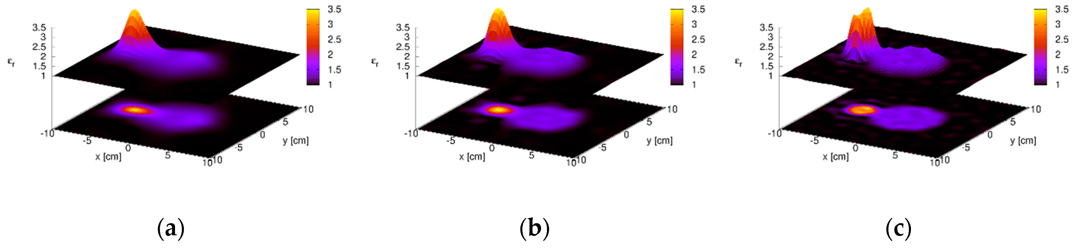
The reconstructed distribution of the relative dielectric permittivity for some of the available working frequencies are shown in Figure 2. The results obtained with the optimal value of the norm parameter are reported in the first row, whereas the corresponding Hilbert-space reconstructions are provided for comparison in the second row. As can be seen, the Lebesgue-space method is able to reconstruct correctly the inspected scenario in all cases, providing a quite accurate reconstruction of the cylinders’ cross section, both in terms of dimensions and dielectric permittivity. Using the Hilbert-space procedure it still is possible to identify both targets, but a significant over-smoothing effect is present (which prevents a good reconstruction of the small cylinder) and the ringing in the background is higher. This basic numerical example confirms the behavior of the inversion procedure in Lebesgue spaces, with respect to different choices of the exponent parameter, as briefly discussed at the end of the previous Subsection. Indeed, in Figure 2d–f, where , oversmooting effects are quite evident, whilst in Figure 2a–c, where and 1.3, the reconstructions are less oversmoothed (but some numerical instabilities may occur, especially for smaller , not shown here). These two kinds of results usually are associated with too high and too low regularization in classical Tikhonov Hilbertian approaches, respectively.
Such considerations are also supported by the values of the mean relative errors reported in Table 1, defined as:
where denotes the reconstructed dielectric permittivity, and , are the subdomains occupied by the target and by the background, respectively.
Table 1 also reports the computational data for the considered cases (on a computer equipped with an Intel i5-8265u CPU and 16 GB of RAM). Specifically, the numbers of performed outer iterations, , and the corresponding average computational time per iteration, , are provided. As expected, the time needed for performing a single outer iteration is similar between the optimal norm and the Hilbert-space approaches. However, in all cases, less iterations are needed when considering the optimal Lebesgue-space procedure, allowing a faster reconstruction.
It is worth remarking that the over-smoothing effect in the Hilbert-space solution can be reduced by varying the regularization parameter, which in the present approach is represented by the number of iterations. Table 2 reports the reconstruction errors obtained with different values of the parameters in the case (the threshold on the is not set). As can be seen, the object error decreases when higher values of are used (i.e., a lower regularization is performed), becoming comparable with the ones provided by the optimal value of the norm parameter (in particular, the peak value of the dielectric permittivity is closer). However, the background error increases significantly, producing a greater overall reconstruction error.
As an example, Figure 3 shows the mean relative reconstruction errors versus the norm parameter for the case of the lowest frequency (i.e., ). The overall reconstruction error presents a minimum value corresponding to the optimal norm parameter . Following that, the error increases monotonically with . Moreover, as expected, the background error is always increasing, since low values of produce sparser solutions. Concerning the object error, in this case a minimum is present at , and after an initial increase it becomes almost constant. Similar trends can be observed for the other frequencies. To summarize, Figure 4 shows the behavior of the residual functional (Figure 4a) and of the normalized root mean square error (Figure 4b) versus the outer iteration number for the case . As can be seen, for all values of the algorithm converges after few iterations (between 5 and 8).
4. Multifrequency Lebesgue-Space Inversion
To increase the available information, multi-frequency data can be exploited. It is assumed to have at our disposal the scattered-field data collected for a set of values of the angular frequencies , . Subsequently, a subscript is added to the frequency-dependent functions and operators to specify at which frequency they refer. However, since the contrast function depends upon the frequency, it is necessary to modify the problem formulation [31,41]. To explain, let us assume that the dielectric permittivity and the electric conductivity do not depend on the frequency (i.e., dispersion is neglected). The contrast function in this case can be rewritten as:
where is a reference frequency and the new unknown, which does not depend on the frequency, is given by . The inverse scattering problem at a single frequency can be then described by the following equation:
where is given by (4).
It is worth noting that now is a real-valued function, whereas the electric fields are complex-valued. To work with all real-valued functions, the data are split into their real () and imaginary () parts. Applying (25) to all the available frequencies and stacking all the resulting functional equations, the multi-frequency operator equation to be inverted can be then formally written as:
Concerning the Fréchet derivative of the new operator, needed in the outer linearization step, it can be written in terms of the derivative of the complex single-frequency operator as:
with
It is worth remarking that the multifrequency inversion technique is based on the use of the Lebesgue-space theory discussed in Section 3. Consequently, the same value of the norm parameter is used for all the elements of the data vector (i.e., the scattered fields at the different frequencies). A possible future extension of the approach would be to use different values of for the different frequencies (i.e., for different parts of the data vector) by exploiting the variable-exponent Lebesgue space theory discussed in Section 5.
A Reconstruction Example
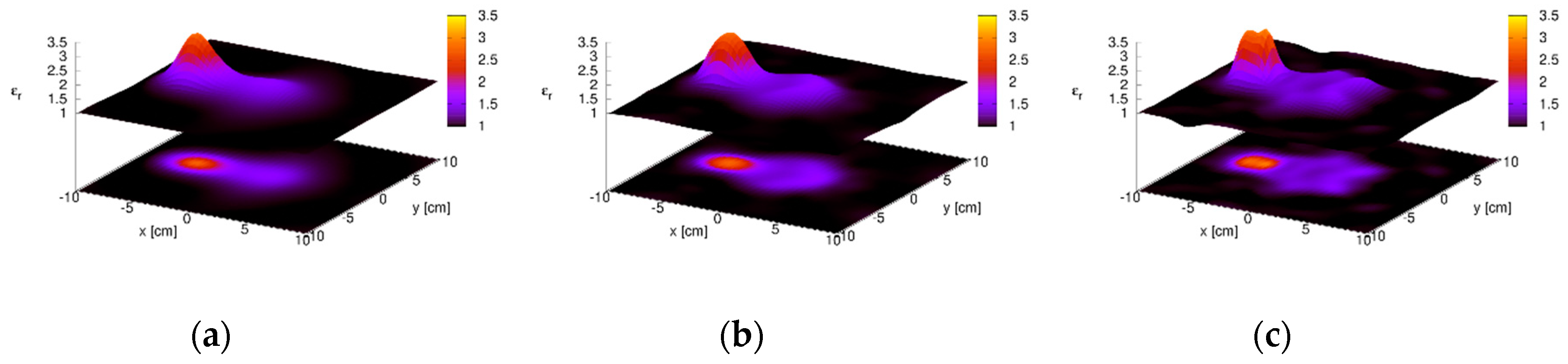
To show the effectiveness of the multi-frequency approach combined with the Lebesgue-space inversion procedure, the FoamDielExtTM target considered in Section 3.4 has been used again as a reference target. As previously described, the Fresnel data are available in the range 2–10 GHz. Consequently, the frequencies considered in the inversion are , . Figure 5 shows the results obtained by considering , , and . As can be seen, increasing the number of processed data allows one to improve the reconstruction quality with respect to the single-frequency inversion procedure, especially concerning the edges of the two cylinders. This improvement is also confirmed by the reconstruction errors reported in Table 3. As expected, all the reconstruction errors decrease when increases, although for higher than about 5 a slower improvement can be observed. Even in this case, the use of a norm with an exponent lower than 2 always produces better reconstructions than the corresponding standard Hilbert-space approach. However, when a high number of frequencies are used, the advantages of using lower exponent parameters become less significant (although always present). It is worth remarking that, in this case, the Hilbert-space approach could provide results comparable to the optimal Lebesgue-space procedure by considering a higher number of frequencies. As an example, the reconstruction errors obtained with the Hilbert-space approach with 7 frequencies are comparable to the ones of the optimal Lebesgue-space procedure with 4 frequencies. However, the computational cost is significantly higher (the needed time per iteration is doubled and the number of iterations is three times higher). Concerning the computational times, it should also be noted that in the multifrequency case they are higher than the single-frequency case and increase with the number of processed frequencies. Such an increase is due to the higher dimensions of the involved matrices. Moreover, in the current implementation, several sub-matrix and sub-vector extractions are performed for building the Fréchet derivative in (27)–(28), leading to an additional computational burden.
5. The Novel Variable-Exponent Approach
To summarize, the inverse scattering results obtained by using the inexact Newton method as a regularization algorithm for the nonlinear Equation (5) in some Lebesgue spaces show less presence of over-smoothing in the reconstructed properties of the targets. Naturally, this is an interesting property for all the applications in which an accurate dielectric reconstruction is required. Despite these advantages, a critical issue should be tackled, related to the selection of the value of that gives rise to the best results. This parameter is essential, since it allows the definition of the space in which the algorithm operates and, thus, the corresponding norm. Confirmed by heuristic analyses, it turns out that the background of a dielectric reconstruction obtained by an -space inversion with low values of the exponent is cleaner from ringing effects. Additionally, discontinuities in the dielectric properties of the targets are retrieved with a higher level of accuracy. Conversely, values of are more suitable for reconstructing the internal part of scatterers with homogeneous dielectric characteristics. Taking the point of view of applications, a sort of compromise between these trends has to be found. Some indications have been derived from numerical and experimental analyses, in which this parameter has been studied with regard to different target typologies, their dielectric properties, size, and the amount of data signal-to-noise ratio [30,41]. Despite this, with the tools described so far, only an a-posteriori selection of the optimal has been done. Clearly, such an optimal choice is feasible only in controlled conditions, when the actual solution is known.
To overcome such a limitation, an innovative approach working in Lebesgue spaces (i.e., where the exponent is a non-constant function) has been recently devised in [42]. The key point of this method is the possibility to have a variable parameter in the investigation domain, which is not limited anymore to be a unique constant value. The considered functional spaces are different from the Lebesgue spaces of -integrable functions (in which is constant) and the power turns out to be a function of the position, in other words. The result is the freedom of defining a different value of for each point inside the region under inspection: This way, the sparsity of the background can be enforced with low values of , whereas values of closer to 2 can be used to achieve a more accurate reconstruction of the properties inside the scatterers.
The price to pay is a more complex mathematical structure of the Lebesgue spaces with variable exponents compared to the Lebesgue spaces (i.e., with constant exponent). An example is the computation of the -space norm. First, to calculate the norm, the evaluation of the modulus is necessary, i.e.:
which generalizes the argument of the (constant-value) -root of (21) to an exponent function , [42]. The -root is required in the definition (21) for guaranteeing that the homogeneity property of any norm holds, that is for any real value . Moreover, the -root of the constant case cannot be directly extended to the non-constant case, because there is not a unique value to use. The -norm, which extends the -space definition (21) and also is known as a Luxemburg norm [42], is found, thus, by solving a one-dimensional minimization problem, that is:
When the exponent is a constant value (denoted as ), it clearly results that:
where the identity holds only in this constant case (otherwise it cannot be formally written).
Considering the above concepts, the extension of the Landweber-type iterations in (20) to the variable-exponent Lebesgue space relies on the calculation of the -space duality maps and has the following form:
where and are the duality maps of and , and the function represents the Hölder conjugate of , defined as . This iterative algorithm, although formally similar to (20), has relevant differences inside the expression of the duality map , which is now defined as:
This expression has been found by exploiting the Fréchet derivative of the norm in spaces [43] and needs to evaluate the Luxemburg norm (30) of . Taking a purely theoretical point of view, it is important to note that, differing from the conventional constant exponent case, the duality map is only an approximation of the respective duality map of the dual space of which is used in the iterative scheme.
5.1. Strategies for Choosing the Variable Exponent Function
The possibility of arbitrarily selecting the exponent , which is a function with values , can be exploited to apply different exponent parameters to different regions of the investigation domain. However, the choice of such a function has not been discussed yet in this survey. The basic idea behind our proposal has been explained in the previous subsection: Exponents close to 1 are useful in the background (to improve the sparsity and reduce the ringing phenomena), while exponents close to 2 are useful inside the scattering objects (to estimate the true values of their dielectric distribution). Although background and location of the objects are not known as prior information, but rather their retrieval is the aim of the proposed algorithms, an estimate can be obtained by the first iterations of any classical methodology. This way, we can consider the first reconstruction (even if really poor) as basic information for constructing the exponent function for the space of unknown . Concerning the data space , the norm parameter is kept constant and equal to the average value of , .
Based on this paradigm, we have developed an adaptive and automatic iterative procedure for defining the nonconstant exponent . An improved accuracy, as well as a greater stability compared to reconstruction algorithms in constant-exponent spaces, characterize the novel procedure. To detail more, a map of the values of , for , is updated at each Newton iteration on the basis of the retrieved values of the contrast function inside the investigation domain . The exponent function is chosen such that (with and ), where and are two values fixed before starting the inversion process, which identify the range of variation. The update equation of the exponent is given by:
in which denotes the current inexact-Newton iteration. The mapping function has values from to and presents a monotonic increase. The application of (34) results in a non-linear scaling of the values of the contrast function magnitude (divided by its maximum value) in the given interval range for the exponents, . Since the background region (i.e., the set of points of where no targets are present) is characterized by low values of , the corresponding values of given by (34) will approach the minimum of the range . In this way, the region outside targets would present a reduction of background ringing and artifacts. Conversely, in the regions internal to the scattering targets (where is close to its maximum) will approach , providing a good retrieval of the properties of large regions without overestimation peaks.
Equation (34) defines by exploiting the reconstructed contrast function, which is typically available after the first outer step of the inexact-Newton loop. To start the inexact-Newton iterations, different strategies can be followed based on the availability of a-priori information. When an initial guess is available before executing the inversion (that is, we know a starting approximate solution ), (34) can still be applied considering such an estimated value of the unknown. Alternatively, when this kind of information is not available, a constant function can be considered, obtaining the same initial iteration as the fixed-exponent approach (20).
5.2. A Reconstruction Example
To give an example, the FoamDielExtTM target considered in Section 3.4 has been reconstructed by using the variable-exponent approach. The parameters of the outer and inner loops are the same as in the constant exponent case. The power function has been defined with and . Five different typologies of mapping functions are experimented:
- Linear →
- Square →
- Square root →
- Arcsin →
- Sine →
The reconstruction results are summarized in Table 4, which reports the reconstruction errors obtained with the variable-exponent procedure when considering the data at 2, 3 and 4 GHz. Regarding this configuration, the different mapping functions provide comparable errors. Moreover, the obtained results are similar to the ones provided by the optimal norm parameter in the fixed-exponent algorithm. The corresponding computational times are reported in Table 5. As can be seen, the time needed for performing a single outer iteration is only slightly higher than the corresponding time for the fixed exponent case (see Table 1). Such a small increase is due to the increased complexity in the computation of the Luxemburg norm. However, the number of needed iterations is still comparable to the fixed-exponent case, thus the overall computational burden is only slightly greater. It is worth remarking that, although the reconstruction quality (both in terms of computational cost and errors) is comparable, the main advantages of the proposed variable approach are related to the fact that it does not require an a-priori selection of the norm parameter , whose optimal value can be selected only a-posteriori and with some knowledge of the expected results. Actually, the user is only required to select a range of values for this parameter, whose choice is far less critical. Figure 6 shows the reconstructed distribution of the relative dielectric permittivity for a linear mapping function. Observing the results, we notice a correct retrieval of the properties of both targets. Additionally, the -space reconstructions look very similar to the ones obtained when considering the fixed-exponent method with an optimal choice of the exponent . This is further confirmed by the cuts of the relative dielectric permittivity along the x axis reported in Figure 7.
6. Conclusions
An overview of the recent advancements in the development of microwave imaging methods based on inversion procedures in Lebesgue spaces has been reported. First, an introductory description of the inverse-scattering problem formulation has been provided. Subsequently, the application of Newton-based techniques combined with regularization strategies in Hilbert and fixed-exponent Lebesgue spaces has been reviewed, including multi-frequency approaches. Next, the more recent variable-exponent space methods have been detailed. The adaptive procedure used to define, iteration by iteration, the power function of the variable-exponent spaces removes the need for choosing a fixed space exponent value. Previously, the choice of the “best” fixed exponent was possible only with an a-posteriori error analysis, based on known configurations. Therefore, the applicability of this kind of inversion methods in real environments is now significantly increased, in particular when no a-priori information about the target is available. The considered inversion techniques have been analyzed and compared by considering experimental data, confirming their effectiveness also under realistic operating conditions.
Author Contributions
Conceptualization, C.E., A.F., M.P., and A.R.; methodology, C.E., A.F., M.P., and A.R.; formal analysis, C.E., A.F., M.P., and A.R.; investigation, C.E., A.F., M.P., and A.R.; validation, C.E., A.F., M.P., and A.R.
Funding
This research was partly supported by the Italian Ministry for Education, University, and Research under the project PRIN2015 U-VIEW, grant number 20152HWRSL. The work of C. Estatico was partly supported by GNCS-INdAM, Italy.
Conflicts of Interest
The authors declare no conflict of interest.
References
- Nikolova, N.K. Introduction to Microwave Imaging; Cambridge University Press: Cambridge, UK, 2017; ISBN 978-1-316-08426-7. [Google Scholar]
- Chen, X. Computational Methods for Electromagnetic Inverse Scattering; John Wiley & Sons: South Tower, Singapore, 2018. [Google Scholar]
- Vacca, M.; Tobon, J.A.; Pulimeno, A.; Sarwar, I.; Vipiana, F.; Casu, M.R.; Solimene, R. A COTS-Based Microwave Imaging System for Breast-Cancer Detection. IEEE Trans. Biomed. Circuits Syst. 2017, 11, 804–814. [Google Scholar] [Green Version]
- Brancaccio, A.; Leone, G.; Solimene, R. Single-frequency subsurface remote sensing via a non-cooperative source. J. Electromagn. Waves Appl. 2016, 30, 1147–1161. [Google Scholar] [CrossRef]
- Coli, V.L.; Tournier, P.; Dolean-Maini, V.; Kanfoud, I.E.; Pichot, C.; Migliaccio, C.; Blanc-Féraud, L. Detection of Simulated Brain Strokes Using Microwave Tomography. IEEE J. Electromagn. RF Microwaves Med. Biol. 2019, 1. [Google Scholar] [CrossRef]
- Solimene, R.; Soldovieri, F.; Prisco, G.; Pierri, R. Three-Dimensional Through-Wall Imaging Under Ambiguous Wall Parameters. IEEE Trans. Geosci. Remote. Sens. 2009, 47, 1310–1317. [Google Scholar] [CrossRef]
- Pastorino, M.; Randazzo, A. Microwave Imaging Methods and Applications; Artech House: Norwood, MA, USA, 2018; ISBN 978-1-63081-348-2. [Google Scholar]
- Burfeindt, M.J.; Shea, J.D.; Van Veen, B.D.; Hagness, S.C. Beamforming-Enhanced Inverse Scattering for Microwave Breast Imaging. IEEE Trans. Antennas Propag. 2014, 62, 5126–5132. [Google Scholar] [CrossRef] [PubMed]
- Zoughi, R. Microwave Non-Destructive Testing and Evaluation; Kluwer Academic Publishers: Dordrecht, The Newtherlands, 2000; ISBN 0-412-62500-8. [Google Scholar]
- Bevacqua, M.; Crocco, L.; Di Donato, L.; Isernia, T.; Palmeri, R. Exploiting sparsity and field conditioning in subsurface microwave imaging of nonweak buried targets. Radio Sci. 2016, 51, 301–310. [Google Scholar] [CrossRef] [Green Version]
- Frezza, F.; Pajewski, L.; Ponti, C.; Schettini, G. Through-wall electromagnetic scattering by N conducting cylinders. J. Opt. Soc. Am. A 2013, 30, 1632–1639. [Google Scholar] [CrossRef] [PubMed]
- Palmeri, R.; Bevacqua, M.T.; Crocco, L.; Isernia, T.; Di Donato, L. Microwave Imaging via Distorted Iterated Virtual Experiments. IEEE Trans. Antennas Propag. 2017, 65, 829–838. [Google Scholar] [CrossRef]
- Solimene, R.; Leone, G. MUSIC Algorithms for Grid Diagnostics. IEEE Geosci. Remote. Sens. Lett. 2013, 10, 226–230. [Google Scholar] [CrossRef]
- Solimene, R.; Soldovieri, F.; Prisco, G. A Multiarray Tomographic Approach for Through-Wall Imaging. IEEE Trans. Geosci. Remote. Sens. 2008, 46, 1192–1199. [Google Scholar] [CrossRef]
- Zhong, Y.; Lambert, M.; Lesselier, D.; Chen, X. A new integral equation method to solve highly nonlinear inverse scattering problems. IEEE Trans. Antennas Propag. 2016, 64, 1788–1799. [Google Scholar] [CrossRef]
- Shumakov, D.S.; Nikolova, N.K. Fast Quantitative Microwave Imaging With Scattered-Power Maps. IEEE Trans. Microwave. Theory Tech. 2018, 66, 439–449. [Google Scholar] [CrossRef]
- Shah, P.; Khankhoje, U.K.; Moghaddam, M. Inverse scattering using a joint L1–L2 norm-based regularization. IEEE Trans. Antennas Propag. 2016, 64, 1373–1384. [Google Scholar] [CrossRef]
- Taskin, U.; Ozdemir, O. Sparsity Regularized Nonlinear Inversion for Microwave Imaging. IEEE Geosci. Remote. Sens. Lett. 2017, 14, 2220–2224. [Google Scholar] [CrossRef]
- Salucci, M.; Oliveri, G.; Anselmi, N.; Viani, F.; Fedeli, A.; Pastorino, M.; Randazzo, A. Three-dimensional electromagnetic imaging of dielectric targets by means of the multiscaling inexact-Newton method. J. Opt. Soc. Am. A 2017, 34, 1119–1131. [Google Scholar] [CrossRef] [PubMed]
- Azghani, M.; Marvasti, F. L2-regularized Iterative Weighted Algorithm for Inverse Scattering. IEEE Trans. Antennas Propag. 2016, 64, 2293–2300. [Google Scholar] [CrossRef]
- Rabbani, M.; Tavakoli, A.; Dehmollaian, M. A Hybrid Quantitative Method for Inverse Scattering of Multiple Dielectric Objects. IEEE Trans. Antennas Propag. 2016, 64, 977–987. [Google Scholar] [CrossRef]
- Gilmore, C.; Abubakar, A.; Hu, W.; Habashy, T.M.; van den Berg, P.M. Microwave biomedical data inversion using the finite-difference contrast source inversion method. IEEE Trans. Antennas Propag. 2009, 57, 1528–1538. [Google Scholar] [CrossRef]
- De Zaeytijd, Jü.; Franchois, A.; Eyraud, C.; Geffrin, J.-M. Full-wave three-dimensional microwave imaging with a regularized Gauss–Newton method–Theory and experiment. IEEE Trans. Antennas Propag. 2007, 55, 3279–3292. [Google Scholar] [CrossRef]
- Bisio, I.; Fedeli, A.; Lavagetto, F.; Pastorino, M.; Randazzo, A.; Sciarrone, A.; Tavanti, E. A numerical study concerning brain stroke detection by microwave imaging systems. Multimedia Tools Appl. 2018, 77, 9341–9363. [Google Scholar] [CrossRef]
- Abubakar, A.; Habashy, T.M.; Pan, G.; Li, M.-K. Application of the Multiplicative Regularized Gauss–Newton Algorithm for Three-Dimensional Microwave Imaging. IEEE Trans. Antennas Propag. 2012, 60, 2431–2441. [Google Scholar] [CrossRef]
- Pastorino, M. Stochastic Optimization Methods Applied to Microwave Imaging: A Review. IEEE Trans. Antennas Propag. 2007, 55, 538–548. [Google Scholar] [CrossRef]
- Schuster, T.; Kaltenbacher, B.; Hofmann, B.; Kazimierski, K.S. Regularization Methods in Banach Spaces; De Gruyter: Berlin, Germany, 2012; ISBN 978-3-11-025524-9. [Google Scholar]
- Schopfer, F.; Louis, A.K.; Schuster, T. Nonlinear iterative methods for linear ill-posed problems in Banach spaces. Inverse Prob. 2006, 22, 311–329. [Google Scholar] [CrossRef] [Green Version]
- Hein, T.; Kazimierski, K.S. Accelerated Landweber iteration in Banach spaces. Inverse Prob. 2010, 26. [Google Scholar] [CrossRef]
- Estatico, C.; Pastorino, M.; Randazzo, A. A Novel Microwave Imaging Approach Based on Regularization in Lp Banach Spaces. IEEE Trans. Antennas Propag. 2012, 60, 3373–3381. [Google Scholar] [CrossRef]
- Estatico, C.; Fedeli, A.; Pastorino, M.; Randazzo, A. A Multi-Frequency Inexact-Newton Method in Lp Banach Spaces for Buried Objects Detection. IEEE Trans. Antennas Propag. 2015, 63, 4198–4204. [Google Scholar] [CrossRef]
- Estatico, C.; Pastorino, M.; Randazzo, A.; Tavanti, E. Three-Dimensional Microwave Imaging in Lp Banach Spaces: Numerical and Experimental Results. IEEE Trans. Comput. Imaging 2018, 4, 609–623. [Google Scholar] [CrossRef]
- Estatico, C.; Fedeli, A.; Pastorino, M.; Randazzo, A. Buried object detection by means of a Lp Banach-space inversion procedure. Radio Sci. 2015, 50, 41–51. [Google Scholar] [CrossRef]
- Estatico, C.; Fedeli, A.; Pastorino, M.; Randazzo, A. Quantitative Microwave Imaging Method in Lebesgue Spaces With Nonconstant Exponents. IEEE Trans. Antennas Propag. 2018, 66, 7282–7294. [Google Scholar] [CrossRef]
- Quarteroni, A.; Sacco, R.; Saleri, F. Numerical Mathematics, 2nd ed.; Springer: Berlin, Germany, 2006; ISBN 978-3-540-34658-6. [Google Scholar]
- Boccacci, P.; Bertero, M. Introduction to Inverse Problems in Imaging; CRC Press: Boca Raton, FL, USA, 1998. [Google Scholar]
- Bozza, G.; Pastorino, M. An Inexact Newton-Based Approach to Microwave Imaging Within the Contrast Source Formulation. IEEE Trans. Antennas Propag. 2009, 57, 1122–1132. [Google Scholar] [CrossRef]
- Randazzo, A.; Oliveri, G.; Massa, A.; Pastorino, M. Electromagnetic inversion with the multiscaling inexact Newton method–experimental validation. Microwave. Opt. Technol. Lett. 2011, 53, 2834–2838. [Google Scholar] [CrossRef]
- Belkebir, K.; Saillard, M. Testing inversion algorithms against experimental data: inhomogeneous targets. Inverse Prob. 2005, 21, S1–S3. [Google Scholar] [CrossRef]
- Geffrin, J.-M.; Sabouroux, P.; Eyraud, C. Free space experimental scattering database continuation: experimental set-up and measurement precision. Inverse Probl. 2005, 21, S117–S130. [Google Scholar] [CrossRef]
- Estatico, C.; Fedeli, A.; Pastorino, M.; Randazzo, A. A Banach Space Regularization Approach for Multifrequency Microwave Imaging. Int. J. Antennas Propag. 2016, 2016, 1–8. [Google Scholar] [CrossRef] [Green Version]
- Diening, L.; Harjulehto, P.; Hästö, P.; Ruzicka, M. Lebesgue and Sobolev Spaces with Variable Exponents; Springe: Berlin, Germany, 2011. [Google Scholar]
- Dinca, G.; Matei, P. Geometry of Sobolev spaces with variable exponent: smoothness and uniform convexity. C. R. Math. 2009, 347, 885–889. [Google Scholar] [CrossRef]
Figure 1.
Schematic representation of a generic microwave imaging configuration.

Figure 2.
Reconstructed distribution of the relative dielectric permittivity. FoamDielExtTM target. Upper row: Lebesgue-space inversion for (a) (), (b) (), and (c) (). Lower row: Hilbert-space inversion (i.e., ) for (d) , (e) , and (f) .
Figure 2.
Reconstructed distribution of the relative dielectric permittivity. FoamDielExtTM target. Upper row: Lebesgue-space inversion for (a) (), (b) (), and (c) (). Lower row: Hilbert-space inversion (i.e., ) for (d) , (e) , and (f) .

Figure 3.
Mean relative reconstruction errors (overall, target and background only) versus the norm parameter . . Lebesgue-space inversion.
Figure 3.
Mean relative reconstruction errors (overall, target and background only) versus the norm parameter . . Lebesgue-space inversion.

Figure 4.
Residual (a) and normalized root mean square error (b) versus the outer (Newton) iteration number and for several values of the norm parameter . . Lebesgue-space inversion.
Figure 4.
Residual (a) and normalized root mean square error (b) versus the outer (Newton) iteration number and for several values of the norm parameter . . Lebesgue-space inversion.

Figure 5.
Reconstructed distribution of the relative dielectric permittivity: (a) frequencies (2–3 GHz); (b) frequencies (2–5 GHz); (c) frequencies (2–7 GHz). FoamDielExtTM target. Multi-frequency Lebesgue-space approach.
Figure 5.
Reconstructed distribution of the relative dielectric permittivity: (a) frequencies (2–3 GHz); (b) frequencies (2–5 GHz); (c) frequencies (2–7 GHz). FoamDielExtTM target. Multi-frequency Lebesgue-space approach.

Figure 6.
Reconstructed distribution of the relative dielectric permittivity for (a) , (b) , and (c) . Variable-exponent Lebesgue-space approach.
Figure 6.
Reconstructed distribution of the relative dielectric permittivity for (a) , (b) , and (c) . Variable-exponent Lebesgue-space approach.

Figure 7.
Cuts along the line of the reconstructed distributions of the relative dielectric permittivity for (a) , (b) , and (c) . Variable-exponent Lebesgue-space approach.
Figure 7.
Cuts along the line of the reconstructed distributions of the relative dielectric permittivity for (a) , (b) , and (c) . Variable-exponent Lebesgue-space approach.


Table 1.
Reconstruction errors, outer iteration numbers, and computational times. Lebesgue-space inversion.
Table 1.
Reconstruction errors, outer iteration numbers, and computational times. Lebesgue-space inversion.
| Frequency [GHz] | Lebesgue (Optimal Norm) | Hilbert | |||||||||
|---|---|---|---|---|---|---|---|---|---|---|---|
| popt | einv | eobj | ebg | tm [s] | einv | eobj | ebg | tm [s] | |||
| 2 | 1.2 | 0.060 | 0.14 | 0.047 | 5 | 11.78 | 0.11 | 0.16 | 0.098 | 6 | 12.54 |
| 3 | 1.3 | 0.082 | 0.13 | 0.074 | 10 | 17.26 | 0.12 | 0.13 | 0.12 | 12 | 16.93 |
| 4 | 1.3 | 0.096 | 0.13 | 0.091 | 8 | 18.62 | 0.16 | 0.15 | 0.17 | 21 | 21.50 |
Table 2.
Reconstruction errors for different values of the number of inner iterations KLW. . Lebesgue-space inversion.
Table 2.
Reconstruction errors for different values of the number of inner iterations KLW. . Lebesgue-space inversion.
| KLW | einv | eobj | ebg |
|---|---|---|---|
| 25 | 0.13 | 0.16 | 0.13 |
| 50 | 0.14 | 0.15 | 0.14 |
| 75 | 0.14 | 0.15 | 0.14 |
| 100 | 0.14 | 0.14 | 0.14 |
Table 3.
Reconstruction errors, outer iteration numbers, and computational times. Multi-frequency Lebesgue-space approach.
Table 3.
Reconstruction errors, outer iteration numbers, and computational times. Multi-frequency Lebesgue-space approach.
| Number of Frequencies | Lebesgue (Optimal Norm) | Hilbert | |||||||||
|---|---|---|---|---|---|---|---|---|---|---|---|
| popt | einv | eobj | ebg | tm [s] | einv | eobj | ebg | tm [s] | |||
| 2 | 1.3 | 0.057 | 0.12 | 0.047 | 4 | 117.87 | 0.083 | 0.13 | 0.076 | 13 | 133.57 |
| 3 | 1.3 | 0.049 | 0.088 | 0.043 | 6 | 205.97 | 0.066 | 0.098 | 0.061 | 16 | 221.65 |
| 4 | 1.4 | 0.045 | 0.075 | 0.040 | 10 | 313.20 | 0.059 | 0.081 | 0.055 | 21 | 330.66 |
| 5 | 1.4 | 0.041 | 0.066 | 0.036 | 19 | 454.80 | 0.052 | 0.074 | 0.048 | 24 | 451.44 |
| 6 | 1.4 | 0.039 | 0.062 | 0.036 | 17 | 611.34 | 0.049 | 0.071 | 0.045 | 27 | 592.21 |
| 7 | 1.5 | 0.038 | 0.060 | 0.034 | 19 | 772.71 | 0.046 | 0.068 | 0.042 | 28 | 744.73 |
Table 4.
Reconstruction errors. Variable-exponent Lebesgue-space approach.
| Map Type | 2 GHz | 3 GHz | 4 GHz | ||||||
|---|---|---|---|---|---|---|---|---|---|
| einv | eobj | ebg | einv | eobj | ebg | einv | eobj | ebg | |
| Linear | 0.076 | 0.15 | 0.064 | 0.073 | 0.12 | 0.065 | 0.085 | 0.10 | 0.082 |
| Sine | 0.076 | 0.15 | 0.064 | 0.071 | 0.12 | 0.062 | 0.11 | 0.12 | 0.10 |
| Quadratic | 0.079 | 0. 16 | 0.066 | 0.070 | 0.11 | 0.063 | 0.098 | 0.11 | 0.095 |
| Square root | 0.077 | 0.14 | 0.065 | 0.077 | 0.13 | 0.069 | 0.088 | 0.11 | 0.084 |
| Arcsin | 0.077 | 0.15 | 0.066 | 0.078 | 0.12 | 0.070 | 0.092 | 0.11 | 0.090 |
Table 5.
Outer iteration numbers and computational times. Variable-exponent Lebesgue-space approach.
Table 5.
Outer iteration numbers and computational times. Variable-exponent Lebesgue-space approach.
| Map Type | 2 GHz | 3 GHz | 4 GHz | |||
|---|---|---|---|---|---|---|
| tm [s] | tm [s] | tm [s] | ||||
| Linear | 11 | 12.61 | 8 | 17.41 | 6 | 19.05 |
| Sine | 9 | 12.98 | 4 | 16.19 | 8 | 21.80 |
| Quadratic | 7 | 12.74 | 7 | 16.71 | 6 | 18.98 |
| Square root | 11 | 13.06 | 8 | 17.75 | 7 | 19.83 |
| Arcsin | 10 | 12.72 | 8 | 17.59 | 7 | 19.60 |
© 2019 by the authors. Licensee MDPI, Basel, Switzerland. This article is an open access article distributed under the terms and conditions of the Creative Commons Attribution (CC BY) license (http://creativecommons.org/licenses/by/4.0/).
Share and Cite
MDPI and ACS Style
Estatico, C.; Fedeli, A.; Pastorino, M.; Randazzo, A. Microwave Imaging by Means of Lebesgue-Space Inversion: An Overview. Electronics 2019, 8, 945. https://doi.org/10.3390/electronics8090945
AMA Style
Estatico C, Fedeli A, Pastorino M, Randazzo A. Microwave Imaging by Means of Lebesgue-Space Inversion: An Overview. Electronics. 2019; 8(9):945. https://doi.org/10.3390/electronics8090945
Chicago/Turabian StyleEstatico, Claudio, Alessandro Fedeli, Matteo Pastorino, and Andrea Randazzo. 2019. "Microwave Imaging by Means of Lebesgue-Space Inversion: An Overview" Electronics 8, no. 9: 945. https://doi.org/10.3390/electronics8090945
Note that from the first issue of 2016, this journal uses article numbers instead of page numbers. See further details here.