Brick Assembly Networks: An Effective Network for Incremental Learning Problems

Abstract

Deep neural networks have achieved high performance in image classification, image generation, voice recognition, natural language processing, etc.; however, they still have confronted several open challenges that need to be solved such as incremental learning problem, overfitting in neural networks, hyperparameter optimization, lack of flexibility and multitasking, etc. In this paper, we focus on the incremental learning problem which is related with machine learning methodologies that continuously train an existing model with additional knowledge. To the best of our knowledge, a simple and direct solution to solve this challenge is to retrain the entire neural network after adding the new labels in the output layer. Besides that, transfer learning can be applied only if the domain of the new labels is related to the domain of the labels that have already been trained in the neural network. In this paper, we propose a novel network architecture, namely Brick Assembly Network (BAN), which allows a trained network to assemble (or dismantle) a new label to (or from) a trained neural network without retraining the entire network. In BAN, we train labels with a sub-network (i.e., a simple neural network) individually and then we assemble the converged sub-networks that have trained for a single label together to form a full neural network. For each label to be trained in a sub-network of BAN, we introduce a new loss function that minimizes the loss of the network with only one class data. Applying one loss function for each class label is unique and different from standard neural network architectures (e.g., AlexNet, ResNet, InceptionV3, etc.) which use the values of a loss function from multiple labels to minimize the error of the network. The difference of between the loss functions of previous approaches and the one we have introduced is that we compute a loss values from node values of penultimate layer (we named it as a characteristic layer) instead of the output layer where the computation of the loss values occurs between true labels and predicted labels. From the experiment results on several benchmark datasets, we evaluate that BAN shows a strong capability of adding (and removing) a new label to a trained network compared with a standard neural network and other previous work.

1. Introduction

Deep neural networks [1] have played an important role in many areas of artificial intelligence field, such as image classification and object detection [2,3,4,5], image generation [6,7,8,9], speech recognition [10,11,12], text generation [13,14], etc. Although deep neural networks produce remarkable results compared with other machine learning algorithms, there still remain some open challenges for researchers to further investigate. These challenges include incremental learning issue, overfitting, hyperparameter optimization, lack of flexibility and multitasking [15], etc. In this paper, we focus on the issue that a neural network is lacking of flexibility in terms of adding an extra label to its output layer after the neural network has been converged. This is basically one of the incremental learning problems that is related to machine learning methodologies that continuously train an existing model with additional knowledge. The incremental learning problem is worth exploration because most neural network systems have a poor capability in adding new labels to their output layer after the neural network systems have been converged. To the best of our knowledge, there are two common solutions to solve this issue which are ‘retraining’ and ‘transfer learning’ [16]. In the first solution, we add a new data into the training dataset, and we repeat the training procedure on a newly initialized neural network. However, this naïve solution has a drawback, which is that it is very time consuming because we have to retrain the entire neural network every time we add a new label into it. In order to apply a transfer learning on the image classification problem, we remain the convolutional layers of the neural network and retrain only the fully connected layers of the neural network. Although this solution is more effective than the first solution, it has a restriction that the new label must be from a similar domain of the other labels that have already been trained in the neural network.

To address these problems (i.e., time-consuming characteristics of the retraining method and domain restriction limitation of the transfer learning method), we propose a novel network architecture, namely brick assembly network (BAN). From a given dataset regardless its domain, we train each label with a neural network. From now on, we limit our discussion to a widely used convolution neural network (CNN) which consists of an input layer, a convolutional layer, and a fully connected layer to train a label for clear and concise description of our proposed method. We denote this neural network as sub-network for the remaining paragraphs in the paper. After the sub-networks are converged, they are merged together into one full neural network which is called BAN. In short, BAN provides capabilities for labels to be trained in its sub-networks, respectively, to assemble the converged sub-networks to the BAN, or dismantle the sub-networks from the BAN at any time. We explain the capability of BAN more detail in Section 3.2.

In this study, we summarize our research contributions as follows:

• BAN is the first network architecture that provides a capability of a trained neural network to assemble (add) and dismantle (remove) labels without retraining the neural network.
• We introduce a truth labels-less loss function to train a network.
• We propose a way to train a network with only one label data. In other words, we can train BAN with a single label at a time.
• BAN does not include old labels’ datasets during the training phase when we add or remove a label from the network.

To promote reproducible research, we release the implementation of our network architecture (Our scripts are available at https://github.com/canboy123/ban).

2. Related Work

Roy et al. [17] have proposed a hierarchical deep convolutional neural network (TreeCNN) for solving the incremental learning problem by growing a trained network structure if new labels are added to the network. In their experiment results, TreeCNN has shown that it performs lesser training effort than the standard neural network, and it has maintained a competitive accuracy as the standard neural network. However, when new labels are added to a trained TreeCNN, it still requires old data to retrain the network. Besides that, TreeCNN consumes more time to train the network than our BAN as shown in Section 5.

Castro et al. [18] have proposed end-to-end incremental learning model which is composed of a feature extractor and a classification layer. From their experiment results, their model has shown the capability of performing incremental learning by increasing the number of the model’s classification layer when a new label is added into the model. Unlike BAN, they include both new data and old data to train their model during the incremental learning while we just use only the new data to train the sub-network of BAN. Besides that, they do not include the capability of removing a trained label from their model; meanwhile, we show that our BAN can dismantle a label from a trained network.

Rosenblatt [19] is the founder of the perceptron algorithm which is used for supervised learning of binary classifiers. He has introduced an impressive back-propagation procedure for updating the weights of a neural network. Thoroughly, the weights are updated based on the gradient of the loss function in terms of weights. The loss function computes the difference between a true label and a predicted label from a trained network. In this paper, however, we propose a new loss function that updates the weights without using any label which is discussed in Equation (1) of Section 3.2.

Oza and Patel [20] have proposed a novel one-class convolutional neural network. The network has a feature extractor and a classifier. The feature extractor integrates with pseudo-negative class data which are generated from a zero centered Gaussian distribution, and it is used to embed an input image into a feature space. The classifier, however, is used to produce a confidence score (i.e., 1 or 0) for a given input image. Although the authors have shown that their network outperforms other statistical and deep learning-based one class classification methods, it is limited to only one-class case that is either abnormal (1) or normal (0). In BAN, on the other hand, even though our training method of a sub-network is similar to the training method of their model (i.e., train a label in a network), our BAN produces multiple outputs (discussed in Equation (3) of Section 3.2) instead of binary output.

Generally, researchers have proposed a network architecture (e.g., AlexNet [21], GoogLeNet [22], VGGNet [23], etc.) that performs a training which accommodates all procedures from initial random weight assignment to full convergence. In consequence, it is difficult for the network to add a new label to or remove a trained label from the network. Unlike those network architectures, our BAN allows the network to assemble a new trained sub-network or dismantle a trained sub-network from the network without retraining the entire network.

3. Proposed Method

3.1. Preliminaries

Let X be an input image for training neural networks. If the size of the image is $w\times h\times c$, then $\left\{x_i\right|x_i\in X\}$, where $x_i$= $x_1,x_2,\cdots ,x_{w\times h\times c}$ is the pixel of the image. Note that w, h and c refers to width, height and channel, respectively. A classifier $F(·)$ is a function to produce a predicted label $\widehat{Y}$ for X. Let Y be the true label of image X. To optimize a neural network, we minimize a loss function $L(·)$ that computes the difference between a true label Y and a predicted label $\widehat{Y}$ for X. The derivative of the loss function is commonly used for updating the parameters of the neural network such as weights W, biases B, etc.

3.2. Brick Assembly Network

BAN is the novel network architecture that has innovative “retrain-less” features of assembling and dismantling trained sub-networks. In other words, we can add trained sub-networks to a BAN, and also remove trained sub-networks from a BAN without retraining the BAN. Note that the sub-network refers to a network that is trained by feeding only one label data as its training dataset. To compare the performance of BAN with other cutting-edge algorithms, we optimize them by computing the derivatives of their loss functions from several labeled datasets. The training using one label data in BAN is inspired from the observation that the classification step of each label has activated different neural nodes on a penultimate layer (i.e., a fully connected layer before an output layer) of a standard neural network through an activation function. In other words, our observation is that an image with a particular class label produces a unique pattern on the penultimate layer so that the neural network can generate a distinguishable output. To avoid a confusion of addressing the penultimate layer, we called it a characteristic layer that is composed of j nodes, $C\in {\mathbb{R}}^j$, where $j>1$, in the remainder of this paper. Then, $\left\{c_i\right|c_i\in C\}$, where $c_i$ = $c_1$, $c_2$, ⋯, $c_j$ refers to the node value of the characteristic layer. From the characteristic layer, we discover that each label can be trained separately by minimizing a loss function $L_C^l\left(X^l\right)$ defined in Equation (1):

$$\underset{L}{arg\; min}{L}_C^l\left(X^l\right)=\frac{1}{2}{(\widehat{C}-C)}^2$$

(1)

where $L_C(·)$ is a loss function, C is a user-defined characteristic layer composed of j nodes, $\widehat{C}$ is a predicted characteristic layer composed of j nodes, l is a label index, and $X^l$ is an image with a specific label. Note that C is a vector which consists of j values and is initialized with some random values which are $-ϵ\le C_j\le ϵ$, where $ϵ$ is a user-specified threshold. We set $ϵ=5$ in our experiments. We define a simple predicted characteristic layer which is composed of j nodes as shown in Equation (2):

$$\widehat{C}=a(WX+B)$$

(2)

where $a(·)$ is an activation function, W is a weight matrix, X is images, and B is a bias vector.

We illustrate the procedure of training and testing phases of BAN for MNIST (Modified National Institute of Standards and Technology) [24] examples in Figure 1. During the training phase, we train two sub-networks with labeled data (see the blue box in Figure 1), “0” images and “7” images, respectively, by computing the loss function defined in Equation (1). After the sub-networks have converged, we assemble them together to form a BAN as depicted with a red box in the testing phase. To test a new image, we calculate the distances between user-defined values of characteristic layers, C, and predicted values of characteristic layers $\widehat{C}$ in BAN. Then, we classify the image into a specific label which corresponds to the lowest distance as defined in Equation (3):

$$F\left(X\right)=\underset{D}{min}{D}^l({\widehat{C}}^l,C^l)$$

(3)

where $D(·)$ is an Euclidean distance [25], $C^l$ is a user-defined characteristic layer values for a specific label l, ${\widehat{C}}^l$ is a predicted characteristic layer values for a specific label l, l is a label index, and X is an image.

In summary, in order to train a network with only one label data, we optimize the weights of the network by minimizing a loss function from the difference between the values of user-defined characteristic layer C and the values of predicted characteristic layer $\widehat{C}$ which has been shown in Equation (1). This is different from common loss functions which minimize the mean of squared error (MSE) between truth labels and predicted labels with multiple labels data. Hence, we emphasize that our BAN uses a label-less loss function to train a network. Although BAN needs more parameters (i.e., weights) than standard neural networks, it improves the neural network’s capability of adding and classifying new class labels which are either from the same or different domains without retraining the entire network.

3.3. Pseudo-Code of the Brick Assembly Network

We provide Algorithm 1 to explain BAN in terms of pseudo-codes. First, we initialize all weights of convolutional layers and all nodes of characteristic layers to random numbers in the range $[-0.5,0.5]$ and $[-5,5]$, respectively. For each sub-network, we calculate the nodes value of predicted characteristic layer and its loss functions during the feed-forward procedure (in lines 6 to 9 of Algorithm 1). After that, we update the weights W (and biases B) by computing the gradient of the loss function in terms of the weights (in lines 11 to 14 of Algorithm 1). We repeat the feed-forward and back-propagation procedures until the sub-network has converged. Finally, we assemble them to form a BAN.

Algorithm 1. The pseudo-code of the Brick Assembly Network

Input: Image dataset D, distributed into l sub-datasets, where each sub-dataset consists of only one label data, $X^l\subset D$ Output: A converged BAN. 1: Initialization: 2: Initialize the learning rate $\alpha$. 3: Set initial weights $w_1,w_2,\dots ,w_n\in W$ to random numbers in the range [−0.5, 0.5]. 4: Set initial nodes value of characteristic layer $c_1,c_2,\dots ,c_j\in C$ to random numbers $-5\le c_i\le 5$. 5: Feed-forward Procedure: 6: for each neural network do 7:  Compute predicted node values of the characteristic layer of a neural network: $\widehat{C}=h\left(X\right)=a(WX+B)$           ▹$h\left(x\right)$ can be a nested function. 8:  Compute a loss function: $L_C\left(X\right)=\frac{1}{2}{(\widehat{C}-C)}^2$ 9: end for 10: Back-propagation Procedure: 11: for each neural network do 12:  Compute the gradient in terms of weights W: $\frac{\delta L_C\left(X\right)}{\delta W}=(\widehat{C}-C)·\frac{\delta \widehat{C}}{\delta W}$ 13:  Updating weights W: $W=W-\alpha ·\frac{\delta L_C\left(X\right)}{\delta W}$ 14: end for

3.4. Parametric Characteristic Layer

In this paper, we also introduce the parametric characteristic layer. The parametric characteristic layer refers to the node values of a defined characteristic layer C which change dynamically. In other words, the final node values of a defined characteristic layer are different from their initialized values. The purpose of using parametric characteristic layer is to obtain a proper node value of the characteristic layer instead of a fixed node values by using gradient descent with a given parameter vector $\beta$. To produce a parametric characteristic layer, we multiply the characteristic layer C with a parameter vector $\beta$ as defined in Equation (4):

$$C_p={\beta }^{T}C$$

(4)

where $\beta$ is a vector which consists of j parametric variables that control the latency of C. Note that we use the parametric characteristic layer $C_p$ instead of a fixed characteristic layer C in the experiments. Therefore, we modify Equation (1) into Equation (5) and Equation (3) into Equation (6):

$$\underset{L}{arg\; min}{L}_C^l\left(X^l\right)=\frac{1}{2}{(\widehat{C}-{\beta }^{T}C)}^2$$

(5)

$$F\left(X\right)=\underset{D}{min}{D}^l({\widehat{C}}^l,{\beta }^T{C}^l)$$

(6)

We also provide Algorithm 2 to explain the pseudo-code of updating the parametric vector $\beta$.

Algorithm 2. The pseudo-code of the parametric characteristic layer

Input: Image dataset D, distributes into l sub-datasets, each sub-dataset consists of only one label data, $X^l\subset D$ Output: A converged parametric characteristic layer. 1: Initialization: 2: Initialize the learning rate $\alpha$. 3: Set the initial nodes of characteristic layer $c_1,c_2,\dots ,c_j\in C$ with random numbers $-5\le c_i\le 5$. 4: Set the initial trainable weights ${\beta }_1,{\beta }_2,\dots ,{\beta }_j\in \beta$ with random numbers in the range [−0.5, 0.5]. 5: Feed-forward Procedure: 6: Compute predicted node values of the characteristic layer of a neural network: $\widehat{C}=h\left(X\right)=a(WX+B)$ 7: Compute a loss function between a predicted characteristic layer $\widehat{C}$ and parametric characteristic layer $\beta C$: $L_C\left(X\right)=\frac{1}{2}{(\widehat{C}-{\beta }^{T}C)}^2$ 8: Back-propagation Procedure: 9: Compute the gradient of trainable weights, ${\beta }_i$: $\frac{\delta L_C\left(X\right)}{\delta {\beta }_i}=(\widehat{C}-{\beta }^{T}C)·{\nabla }_{{\beta }_i}(\widehat{C}-{\beta }^{T}C)$ 10: Updating trainable weights, ${\beta }_i$: ${\beta }_i={\beta }_{i-1}-\alpha ·\frac{\delta L_C\left(X\right)}{\delta {\beta }_i}$

4. Experiment Settings

Dataset

For experiment analysis of our propose methods, we use three public benchmark datasets in this study. The datasets include MNIST [24], Fashion MNIST [26], and Kuzushiji-MNIST [27]. MNIST, Fashion MNIST, and Kuzushiji-MNIST have 60,000 training images and 10,000 test images associated with labels from ten classes. The size of each image is 28 × 28 grayscale. Note that, in these experiments, we represent the pixel value of the images in a normalized value (i.e., (0, 1)) instead of its original value (i.e., (0, 255)).

We use a basic convolutional neural network (CNN) [21] as the sub-network architecture for each label in three datasets. The sub-network’s architecture is shown in Figure 1. We use one convolutional layer and one fully connected layer (i.e., characteristic layer). The convolutional layers are followed by a Leaky Rectifier Linear Unit (LeakyReLU) [28] activation function.

5. Experiment Results and Discussion

In this study, we perform several experiments to test our proposed network architecture, BAN. In the experiments, we denote $N_{mnist}$, $N_{fmnist}$, and $N_{kmnist}$ as the number of label for MNIST, Fashion MNIST and Kuzushiji-MNIST datasets, respectively. Note that we perform only 50 epochs during the training phase to prevent the network from being over-fitted to the training dataset.

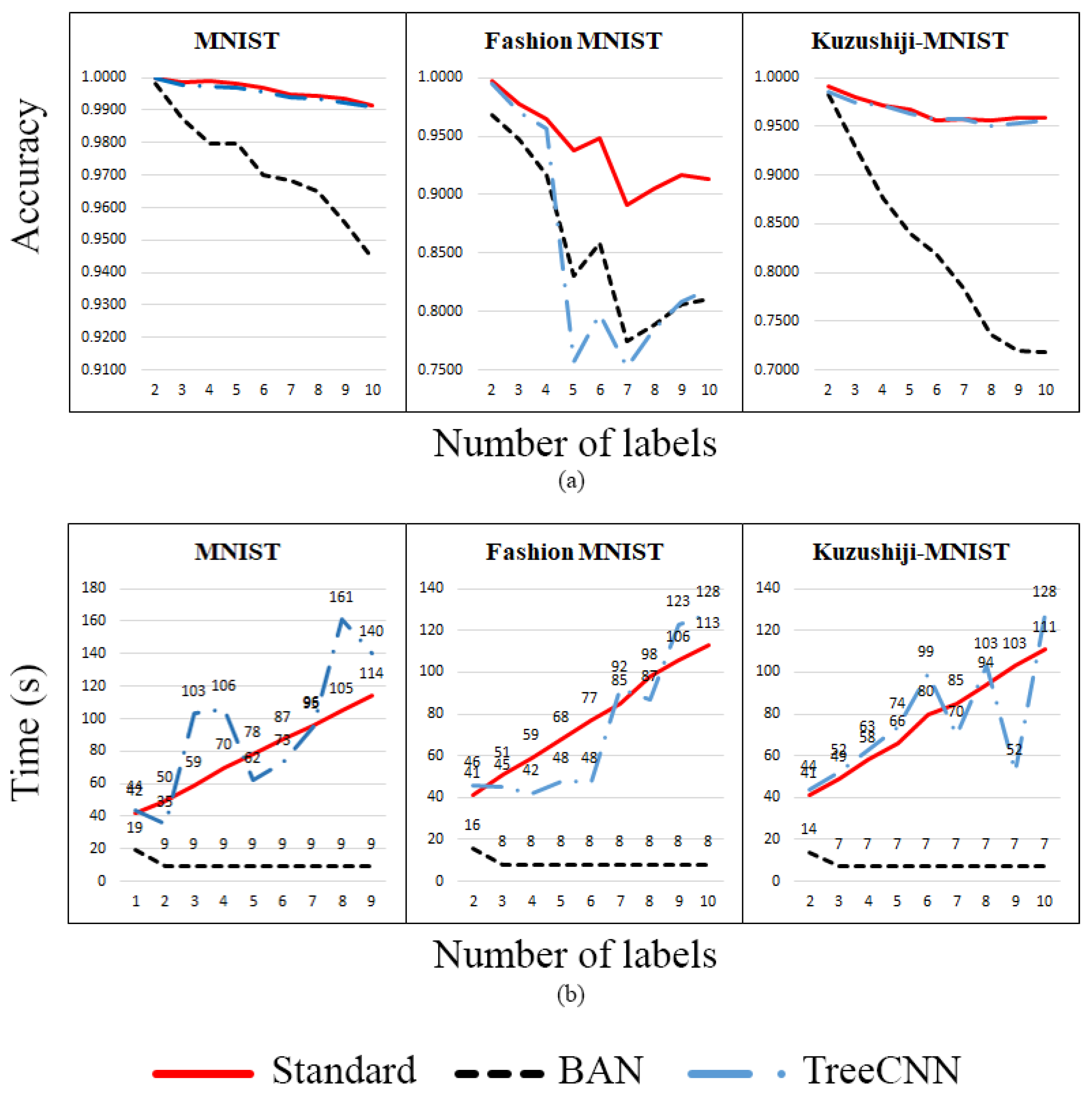
5.1. The Capability of Incrementally Adding New Label(s) on a Trained Network

5.1.1. Single Dataset

The objective of this experiment is to demonstrate the classification performance of the classifiers (i.e., standard neural network, BAN, and TreeCNN [17]) by incrementally adding one new label to each classifier from a given dataset. Each classifier is trained with two labels at the beginning of the experiment. After that, a new label is incrementally added to each classifier until the classifier has trained with ten labels. We illustrate the experiment results in Figure 2. Figure 2a shows the accuracy results of the standard neural network, BAN, and TreeCNN which have trained with different numbers of labels at the 50th epoch. Meanwhile, Figure 2b displays the total time used to train classifiers by incrementally adding one new label to each classifier in 50 epochs. Although BAN produces lower performance than the standard neural network and TreeCNN in terms of accuracy, it has a strong capability of adding (or removing) new labels into a trained network from the observation that the total time used of BAN on training a new label is significantly lesser than the other two networks as shown in Figure 2b. BAN has used less than ten seconds to train each label in MNIST, Fashion MNIST, and Kuzushiji-MNIST, respectively. It is because, unlike the standard neural network and TreeCNN, BAN only has to train a sub-network with the new data without retraining the entire network. Therefore, BAN uses less time to achieve a converged stage.

In the standard image prediction, we apply a softmax function in the output layer of a neural network in order to produce the probability for each neural node. The highest probability of the neural node will be chosen as the final class. In BAN, instead, we compute the distances between user-defined values of parametric characteristic layers, $\beta C$ and predicted values of characteristic layers $\widehat{C}$ as discussed in Equation (6). The lowest distance produced from the particular sub-network will be chosen as the final class. We perform this experiment to evaluate if the distance from Equation (6) can be used for the prediction result. We show the average distance for MNIST, Fashion MNIST, and Kuzushiji-MNIST datasets in

Table 1. The average distance between $\beta C$ and $\widehat{C}$ on each class image of MNIST dataset. Note that the lowest average distance is in bold.

True Label	Predicted Label
	0	1	2	3	4	5	6	7	8	9
0	0.000186	0.007645	0.000471	0.000762	0.000796	0.000489	0.000520	0.001993	0.000610	0.000903
1	0.001541	0.000065	0.000215	0.000376	0.000252	0.000256	0.000426	0.001012	0.000179	0.000555
2	0.000988	0.001925	0.000213	0.000612	0.000867	0.000743	0.000732	0.005793	0.000721	0.001876
3	0.000853	0.001601	0.000367	0.000210	0.001054	0.000345	0.001081	0.001764	0.000463	0.001134
4	0.001074	0.002564	0.000505	0.000553	0.000155	0.000490	0.000866	0.000816	0.000438	0.000615
5	0.000825	0.001596	0.000607	0.000694	0.000759	0.000179	0.000875	0.002095	0.000373	0.001011
6	0.000905	0.003593	0.000469	0.000959	0.000768	0.000756	0.000151	0.009304	0.000868	0.002458
7	0.001447	0.001962	0.001191	0.000452	0.000477	0.000541	0.002470	0.000161	0.000638	0.000412
8	0.000796	0.001359	0.000435	0.000522	0.000540	0.000393	0.000765	0.001318	0.000212	0.000645
9	0.001167	0.001794	0.000797	0.000397	0.000265	0.000379	0.001572	0.000331	0.000371	0.000163

,

Table 2. The average distance between $\beta C$ and $\widehat{C}$ on each class image of Fashion MNIST dataset. Note that the lowest average distance is in bold.

True Label	Predicted Label
	0	1	2	3	4	5	6	7	8	9
0	0.000135	0.001707	0.000247	0.000494	0.000479	0.003169	0.000168	0.101183	0.000382	0.003559
1	0.000329	0.000125	0.000450	0.000336	0.000495	0.001480	0.000391	0.020732	0.000565	0.001418
2	0.000272	0.001305	0.000125	0.000618	0.000231	0.002530	0.000161	0.083569	0.000411	0.003803
3	0.000246	0.000573	0.000298	0.000159	0.000342	0.001338	0.000255	0.024446	0.000432	0.001430
4	0.000272	0.000949	0.000144	0.000449	0.000142	0.001996	0.000151	0.054401	0.000356	0.003784
5	0.001058	0.007484	0.000895	0.002885	0.001812	0.000184	0.000840	0.001232	0.000667	0.000889
6	0.000250	0.001342	0.000203	0.000526	0.000395	0.002419	0.000160	0.059214	0.000387	0.003245
7	0.000718	0.006877	0.000664	0.001859	0.001288	0.000131	0.000617	0.000093	0.000367	0.000430
8	0.000666	0.005456	0.000606	0.001954	0.002104	0.001598	0.000527	0.023552	0.000221	0.003303
9	0.000940	0.006535	0.000878	0.001860	0.002020	0.000275	0.000698	0.000972	0.000468	0.000144

and

Table 3. The average distance between $\beta C$ and $\widehat{C}$ on each class image of Kuzushiji-MNIST dataset. Note that the lowest average distance is in bold.

True Label	Predicted Label
	0	1	2	3	4	5	6	7	8	9
0	0.000278	0.000918	0.000849	0.000477	0.000442	0.000424	0.000719	0.000605	0.000579	0.000553
1	0.000723	0.000238	0.000418	0.000501	0.000403	0.000431	0.000344	0.000590	0.000318	0.000388
2	0.000596	0.000444	0.000297	0.000447	0.000386	0.000399	0.000366	0.000570	0.000384	0.000395
3	0.000555	0.001015	0.000971	0.000265	0.000469	0.000487	0.000527	0.000766	0.000675	0.000626
4	0.000465	0.000527	0.000551	0.000448	0.000293	0.000445	0.000411	0.000598	0.000455	0.000460
5	0.000504	0.000413	0.000469	0.000350	0.000326	0.000168	0.000323	0.000412	0.000314	0.000370
6	0.000672	0.000384	0.000399	0.000446	0.000370	0.000389	0.000227	0.000537	0.000333	0.000433
7	0.000551	0.000734	0.000700	0.000571	0.000484	0.000555	0.000550	0.000488	0.000659	0.000521
8	0.000646	0.000454	0.000527	0.000496	0.000452	0.000469	0.000431	0.000705	0.000253	0.000464
9	0.000572	0.000532	0.000524	0.000527	0.000454	0.000508	0.000532	0.000614	0.000601	0.000299

, respectively. In each table, the first column shows the true label for test images and the remaining columns are the average distance for predicted labels which are generated from sub-networks in BAN. The shortest average distance is in bold. The overall experiment results indicate that BAN has predicted most images correctly except one case in Table 3 with Kuzushiji-MNIST datasets. The exceptional case shows that BAN has predicted most images which are from label 7 to label 4. We believe that the issue can be solved easily by training the sub-network with different loss functions, adding regularizations in the loss function, or applying different activation functions in the layers. We will pursue the study in our future research direction.

5.1.2. Multiple Datasets

The aim of this experiment is to demonstrate the classification performance of three classifiers (i.e., standard neural network, BAN, and TreeCNN) by incrementally adding one new label each from MNIST, Fashion MNIST, and Kuzushiji-MNIST datasets. Initially, the classifier is trained with three labels where each label corresponds to each dataset mentioned above. Following that process, three new labels are incrementally added to the classifier until it becomes trained with total of 30 labels. In other words, we increment the label number of each dataset from one to ten where $N_{mnist},N_{fmnist},N_{kmnist}=\{1,2,3,\dots ,10\}$. We depict the experiment results in Figure 3.

Figure 3a presents the accuracy results of the standard neural network, BAN, and TreeCNN which have been trained with different number of labels at the 50th epoch, whereas Figure 3b shows the total time used to train classifiers by incrementally adding one new label each from the three datasets to each classifier in 50 epochs. Since BAN has trained ten labels from each dataset in Section 5.1.1, then we can use the trained sub-networks directly without any training procedure in this sub-section. Therefore, the total time used to train BAN is 0 for all cases in Figure 3b. Although the accuracy of BAN is lower than the standard neural network and TreeCNN in Figure 3a, we conjecture that it can be increased by using different settings on the sub-network such as the activation function, the number of neural nodes on the characteristic layers C, the user-specified threshold $ϵ$, etc. We will discuss the fine-tuning for the sub-network as our future research directions.

In summary, we evaluate that BAN costs less time to train a new label that is added to the trained network (Section 5.1.1). We also can reuse the trained sub-networks which are trained with different datasets to form one different network structure without any training procedure (Section 5.1.2).

5.2. The Capability of Changing Different Labels on a Network with a Mixture Dataset

The intention of this experiment is to examine the capability of the classifiers (i.e., standard neural network, BAN, and TreeCNN) from the changes of labels while maintaining a fixed number of the labels in the classifier. We perform the experiment with three cases by using two different datasets per case (i.e., MNIST & Fashion MNIST, MNIST & Kujushiji-MNIST, and Fashion MNIST & Kujushiji-MNIST). In each case, we make sure the total number of label chosen from both datasets are equaled to ten (e.g., $N_{mnist}+N_{fmnist}=10$). For example, we select $N_{mnist}=\{1,2,\dots ,9\}$ and $N_{fmnist}=\{9,8,\dots ,1\}$, respectively, in

Table 4. The accuracy of the standard neural network, BAN, and TreeCNN on a mixture dataset of MNIST and Fashion MNIST datasets at the 50th epoch.

# of Label		Accuracy			Retrain			Training Time (s)
${\mathit{N}}_{\mathbf{mnist}}$	${\mathit{N}}_{\mathbf{fmnist}}$	Standard	BAN	TreeCNN	Standard	BAN	TreeCNN	Standard	BAN	TreeCNN
1	9	0.9433	0.8460	0.9165	Yes	No	Yes	121	-	176
2	8	0.9440	0.8550	0.9188	Yes	No	Yes	120	-	178
3	7	0.9652	0.9021	0.9454	Yes	No	Yes	120	-	163
4	6	0.9776	0.9186	0.9588	Yes	No	Yes	126	-	142
5	5	0.9901	0.9551	0.9784	Yes	No	Yes	120	-	143
6	4	0.9911	0.9657	0.9825	Yes	No	Yes	119	-	143
7	3	0.9909	0.9659	0.9837	Yes	No	Yes	123	-	143
8	2	0.9947	0.9708	0.9890	Yes	No	Yes	127	-	143
9	1	0.9933	0.9599	0.9860	Yes	No	Yes	119	-	144

(or the 1st row images of Figure 4). We show the experiment results of three cases in Table 4,

Table 5. The accuracy of the standard neural network, BAN, and TreeCNN on a mixture dataset of MNIST and Kuzushiji-MNIST datasets at the 50th epoch.

# of Label		Accuracy			Retrain			Training Time (s)
${\mathit{N}}_{\mathbf{mnist}}$	${\mathit{N}}_{\mathbf{kmnist}}$	Standard	BAN	TreeCNN	Standard	BAN	TreeCNN	Standard	BAN	TreeCNN
1	9	0.9605	0.7208	0.9226	Yes	No	Yes	115	-	144
2	8	0.9696	0.7541	0.9373	Yes	No	Yes	117	-	146
3	7	0.9792	0.7689	0.9498	Yes	No	Yes	116	-	151
4	6	0.9826	0.7515	0.9560	Yes	No	Yes	111	-	146
5	5	0.9890	0.7793	0.9657	Yes	No	Yes	118	-	146
6	4	0.9921	0.8001	0.9761	Yes	No	Yes	116	-	146
7	3	0.9916	0.8529	0.9765	Yes	No	Yes	117	-	144
8	2	0.9930	0.8958	0.9855	Yes	No	Yes	116	-	152
9	1	0.9940	0.9409	0.9884	Yes	No	Yes	117	-	150

and

Table 6. The accuracy of the standard neural network, BAN, and TreeCNN on a mixture dataset of Fashion MNIST and Kuzushiji-MNIST datasets at the 50th epoch.

# of Label		Accuracy			Retrain			Training Time (s)
${\mathit{N}}_{\mathbf{fmnist}}$	${\mathit{N}}_{\mathbf{kmnist}}$	Standard	BAN	TreeCNN	Standard	BAN	TreeCNN	Standard	BAN	TreeCNN
1	9	0.9616	0.7363	0.9370	Yes	No	Yes	119	-	139
2	8	0.9654	0.7629	0.9428	Yes	No	Yes	122	-	140
3	7	0.9718	0.8025	0.9566	Yes	No	Yes	110	-	140
4	6	0.9667	0.8013	0.9514	Yes	No	Yes	123	-	139
5	5	0.9543	0.7888	0.9375	Yes	No	Yes	119	-	139
6	4	0.9632	0.8169	0.9406	Yes	No	Yes	120	-	142
7	3	0.9277	0.7694	0.8967	Yes	No	Yes	116	-	141
8	2	0.9235	0.8127	0.9023	Yes	No	Yes	117	-	138
9	1	0.9221	0.8223	0.9159	Yes	No	Yes	121	-	141

, respectively. We also illustrate the results of three tables in Figure 4 for a better observation. Although the accuracy of BAN on a mixture of two datasets has lower performance than the standard neural network and TreeCNN, BAN has shown the retrain-less capability of sub-networks since they have been trained in Section 5.1.1. This also shows that the data with only one label can be trained with a unique pattern on the characteristic layer of a neural network. In summary, we evaluate that BAN has the best capability of assembling or dismantling any label to or from BAN while maintaining a fixed number of labels at any time without retraining the network.

5.3. Summary

We provide the qualitative comparison between a standard neural network, BAN, and TreeCNN in

Table 7. The comparison of standard neural network, BAN, and TreeCNN.

	Standard	BAN	TreeCNN
# of Parameters	Low	High	High
Usage of Memory	Low	High	High
Train Individually	Not possible	Possible	Not possible
Re-usability	Not possible	Possible	Not possible
Retraining Time	High	Low/None	High
Old Dataset	Required	Not required	Required
Training Effort [17]	High	Low	Medium
Accuracy	High	Medium	High
Add New Labels	Retrain Entire Network	Train Separately and Merge	Retrain only specific nodes
Requirement in loss function	True Label	Characteristic Layer	True Label

. The ‘number of parameters’ in Table 7 refers to the parameters used in the neural network such as weights, biases, and hyper-parameters of an activation function, etc. Although using BAN requires more memory for storing a high number of parameters, BAN has more advantages than using a standard neural network and TreeCNN. For instance, BAN can train a new label with a sub-network individually and then assemble to a trained BAN. Besides that, the training time of BAN is far lesser than the training time of the standard neural network and TreeCNN because BAN does not require retraining the entire network if new data are added into the dataset. Furthermore, BAN requires no label to train a dataset.

6. Conclusions

In this paper, we propose a novel network architecture, namely BAN which solves the incremental learning problem by assembling or dismantling a trained sub-network to or from a trained BAN. Although BAN consumes more memory, it provides a capability on adding new labels without retrain the network. Moreover, nowadays, computer hardware technology is a rapidly lessening memory issue by increasing the capacity of IC chips. For the future work, we will explore more sub-network settings in order to find the optimal performance configuration for BAN.

References

1. LeCun, Y.; Bengio, Y.; Hinton, G. Deep learning. Nature 2015, 521, 436–444. [Google Scholar] [CrossRef] [PubMed]
2. Chan, T.H.; Jia, K.; Gao, S.; Lu, J.; Zeng, Z.; Ma, Y. PCANet: A simple deep learning baseline for image classification? IEEE Trans. Image Process. 2015, 24, 5017–5032. [Google Scholar] [CrossRef] [PubMed] [Green Version]
3. Li, S.; Song, W.; Fang, L.; Chen, Y.; Ghamisi, P.; Benediktsson, J.A. Deep learning for hyperspectral image classification: An overview. IEEE Trans. Geosci. Remote Sens. 2019, 57, 6690–6709. [Google Scholar] [CrossRef] [Green Version]
4. Perez, L.; Wang, J. The effectiveness of data augmentation in image classification using deep learning. arXiv 2017, arXiv:1712.04621. [Google Scholar]
5. Zhao, W.; Du, S. Spectral–spatial feature extraction for hyperspectral image classification: A dimension reduction and deep learning approach. IEEE Trans. Geosci. Remote Sens. 2016, 54, 4544–4554. [Google Scholar] [CrossRef]
6. Goodfellow, I.; Pouget-Abadie, J.; Mirza, M.; Xu, B.; Warde-Farley, D.; Ozair, S.; Courville, A.; Bengio, Y. Generative adversarial nets. In Proceedings of the Advances in Neural Information Processing Systems Conference, Montreal, QC, Canada, 8–13 November 2014; pp. 2672–2680. [Google Scholar]
7. Mirza, M.; Osindero, S. Conditional generative adversarial nets. arXiv 2014, arXiv:1411.1784. [Google Scholar]
8. Wang, H.; Wang, J.; Wang, J.; Zhao, M.; Zhang, W.; Zhang, F.; Xie, X.; Guo, M. Graphgan: Graph representation learning with generative adversarial nets. In Proceedings of the Thirty-Second AAAI Conference on Artificial Intelligence, New Orleans, LA, USA, 2–7 February 2018. [Google Scholar]
9. Yu, L.; Zhang, W.; Wang, J.; Yu, Y. Seqgan: Sequence generative adversarial nets with policy gradient. In Proceedings of the Thirty-First, AAAI Conference on Artificial Intelligence, San Francisco, CA, USA, 4–9 February 2017. [Google Scholar]
10. Amodei, D.; Ananthanarayanan, S.; Anubhai, R.; Bai, J.; Battenberg, E.; Case, C.; Casper, J.; Catanzaro, B.; Cheng, Q.; Chen, G.; et al. Deep speech 2: End-to-end speech recognition in english and mandarin. In Proceedings of the International Conference on Machine Learning, New York, NY, USA, 20–22 June 2016; pp. 173–182. [Google Scholar]
11. Hannun, A.; Case, C.; Casper, J.; Catanzaro, B.; Diamos, G.; Elsen, E.; Prenger, R.; Satheesh, S.; Sengupta, S.; Coates, A.; et al. Deep speech: Scaling up end-to-end speech recognition. arXiv 2014, arXiv:1412.5567. [Google Scholar]
12. Zhang, Z.; Geiger, J.; Pohjalainen, J.; Mousa, A.E.D.; Jin, W.; Schuller, B. Deep learning for environmentally robust speech recognition: An overview of recent developments. ACM Trans. Intell. Syst. Technol. (TIST) 2018, 9, 1–28. [Google Scholar] [CrossRef]
13. He, X.; Deng, L. Deep learning for image-to-text generation: A technical overview. IEEE Signal Process. Mag. 2017, 34, 109–116. [Google Scholar] [CrossRef]
14. Marcheggiani, D.; Perez-Beltrachini, L. Deep graph convolutional encoders for structured data to text generation. arXiv 2018, arXiv:1810.09995. [Google Scholar]
15. Shrivastava, P. Challenges in Deep Learning. Available online: https://hackernoon.com/challenges-in-deep-learning-57bbf6e73bb (accessed on 10 February 2020).
16. Pan, S.J.; Yang, Q. A survey on transfer learning. IEEE Trans. Knowl. Data Eng. 2009, 22, 1345–1359. [Google Scholar] [CrossRef]
17. Roy, D.; Panda, P.; Roy, K. Tree-CNN: A hierarchical deep convolutional neural network for incremental learning. Neural Netw. 2020, 121, 148–160. [Google Scholar] [CrossRef] [PubMed]
18. Castro, F.M.; Marín-Jiménez, M.J.; Guil, N.; Schmid, C.; Alahari, K. End-to-end incremental learning. In Proceedings of the European Conference on Computer Vision (ECCV), Munich, Germany, 8–14 September 2018; pp. 233–248. [Google Scholar]
19. Rosenblatt, F. The Perceptron, a Perceiving and Recognizing Automaton Project Para; Cornell Aeronautical Laboratory: Buffalo, NY, USA, 1957. [Google Scholar]
20. Oza, P.; Patel, V.M. One-class convolutional neural network. IEEE Signal Process. Lett. 2018, 26, 277–281. [Google Scholar] [CrossRef] [Green Version]
21. Krizhevsky, A.; Sutskever, I.; Hinton, G.E. Imagenet classification with deep convolutional neural networks. In Proceedings of the Advances in Neural Information Processing Systems, Lake Tahoe, NV, USA, 3–6 December 2012; pp. 1097–1105. [Google Scholar]
22. Szegedy, C.; Liu, W.; Jia, Y.; Sermanet, P.; Reed, S.; Anguelov, D.; Erhan, D.; Vanhoucke, V.; Rabinovich, A. Going deeper with convolutions. In Proceedings of the IEEE Conference on Computer Vision and Pattern Recognition, Boston, MA, USA, 7–12 June 2015; pp. 1–9. [Google Scholar]
23. Simonyan, K.; Zisserman, A. Very deep convolutional networks for large-scale image recognition. arXiv 2014, arXiv:1409.1556. [Google Scholar]
24. LeCun, Y.; Bottou, L.; Bengio, Y.; Haffner, P. Gradient-based learning applied to document recognition. Proc. IEEE 1998, 86, 2278–2324. [Google Scholar] [CrossRef] [Green Version]
25. Danielsson, P.E. Euclidean distance mapping. Comput. Graph. Image Process. 1980, 14, 227–248. [Google Scholar] [CrossRef] [Green Version]
26. Xiao, H.; Rasul, K.; Vollgraf, R. Fashion-mnist: A novel image dataset for benchmarking machine learning algorithms. arXiv 2017, arXiv:1708.07747. [Google Scholar]
27. Clanuwat, T.; Bober-Irizar, M.; Kitamoto, A.; Lamb, A.; Yamamoto, K.; Ha, D. Deep learning for classical japanese literature. arXiv 2018, arXiv:1812.01718. [Google Scholar]
28. Maas, A.L.; Hannun, A.Y.; Ng, A.Y. Rectifier nonlinearities improve neural network acoustic models. In Proceedings of the International Conference on Machine Learning, Atlanta, GA, USA, 17–19 June 2013; Volume 30, p. 3. [Google Scholar]
Figure 1. BAN (brick assembly network) architecture with MNIST (Modified National Institute of Standards and Technology) examples.
Electronics 09 01929 g001
Figure 2. Incrementally train a standard neural network, BAN and TreeCNN with MNIST, Fashion MNIST, and Kuzushiji-MNIST datasets at the 50th epoch, respectively. (a) the accuracy of the classifiers; (b) the total time used to train the classifiers. Note that “Standard” refers to the standard neural network.
Electronics 09 01929 g002
Figure 3. Incrementally train a standard neural network, BAN, and TreeCNN with a mixture dataset of MNIST, Fashion MNIST, and Kuzushiji-MNIST datasets at the 50th epoch. (a) the accuracy of the classifiers; (b) the total time used to train the classifiers. Note that “Standard” refers to the standard neural network.
Electronics 09 01929 g003
Figure 4. The performance of the standard neural network, BAN, and TreeCNN on a mixture dataset: (1) MNIST and Fashion MNIST (1st row), (2) MNIST and Kuzushiji-MNIST (2nd row), and (3) Fashion MNIST and Kuzushiji-MNIST (3rd row), at the 50th epoch respectively. (a) Top 3 images from the left show the accuracy of the classifiers; (b) Top 3 images from the right show the total time used to train the classifiers. Note that “Standard” refers to the standard neural network.
Electronics 09 01929 g004