Stereo Vision-Based Object Recognition and Manipulation by Regions with Convolutional Neural Network

Abstract

This paper develops a hybrid algorithm of adaptive network-based fuzzy inference system (ANFIS) and regions with convolutional neural network (R-CNN) for stereo vision-based object recognition and manipulation. The stereo camera at an eye-to-hand configuration firstly captures the image of the target object. Then, the shape, features, and centroid of the object are estimated. Similar pixels are segmented by the image segmentation method, and similar regions are merged through selective search. The eye-to-hand calibration is based on ANFIS to reduce computing burden. A six-degree-of-freedom (6-DOF) robot arm with a gripper will conduct experiments to demonstrate the effectiveness of the proposed system.

1. Introduction

Various types of vision technology, such as image measurement, stereo vision, structured light, time of flight, and laser triangulation are widely used in the field of robotics [1,2]. Due to its superior features in safety, scope, and accuracy, stereo vision is more commonly used. Stereoscopic vision is an imaging technique that compares two images of the same scene and takes object depth from the camera image [3,4,5]. It has been used in industrial automation and applications, for example, box picking and placing, three-dimension (3D) object positioning and recognition, as well as volume measurement [6,7].

Applying stereo vision to a robotic manipulation system typically requires camera calibration and coordinate frame transformation between the stereo camera and the robotic arm. Through MATLAB, the intrinsic and extrinsic parameters required for camera calibration are obtained [1]. The eye-to-hand calibration is used to calculate the relative 3D position and orientation between the camera and the robot arm [8,9]. On identifying objects, there are many techniques for object detection proposed in the literature, for example, sliding window classifiers, pictorial structures, constellation models, and implicit shape models [10]. Sliding window classifiers have been widely used in the fields of detection of faces, pedestrians, and cars because they are especially well suited for rigid objects. Subsequently, the convolutional neural network (CNN) [11,12,13] is one of the most common algorithms. It extracts the image features through the convolutional layer and marks them. The CNN is a special class of neural networks that is best suited for the intelligent processing of visual data. It is a variation of the architecture of a multilayer neural network and generally includes the convolutional layer, pooling layer, flatten layer, fully connected layer, and output layer.

Since a fixed-size frame is used to sweep the entire image one by one, and the size of the target object is unpredictable, it is necessary to use a lot of convolutional layers to perform operations, which result in a longer operation time. As a consequence, the methodology of regions with CNN (R-CNN) [14] is proposed. Regions have not been popular as features due to their sensitivity to segmentation errors. However, region features are appealing because they encode the shape and scale information of objects naturally and are only mildly affected by background clutter [15]. Similar pixels are segmented by the image segmentation method [16], and then the similar regions are merged by selective search [17]. These regions are finally merged into one. The approximate number of frames generated during the merge process is 2000. This method can reduce the amount of input data to speed up the training time. An effective region-based solution for saliency detection is first introduced. Then, the achieved saliency map is applied to better encode the image features for solving object recognition tasks [18]. Superpixels based on an adaptive mean shift algorithm as the basic elements for saliency detection are extracted to find the perceptually and semantically meaningful salient regions. In addition, the Gaussian mixture model (GMM) clustering is used to calculate spatial compactness to measure the saliency of each superpixel. A region-based object recognition (RBOR) method is proposed to identify objects from complex real-world scenes via performing color image segmentation by a simplified pulse-coupled neural network (SPCNN) for the object model image and test image. Then, a region-based matching between them is conducted [19]. Cai et al. [20] proposed a mitosis detection method for breast cancer histopathology images of TUPAC (Tumor Proliferation Assessment Challenge) 2016 and ICPR (International Conference on Pattern Recognition) 2014 datasets by applying the modified R-CNN whose backbone feature extractor is the Resnet-101 network pre-trained on the ImageNet dataset. For traffic surveillance systems, Murugan et al. [21] employed techniques of box filter-based background subtraction to identify the moving objects by smoothing the pixel variations due to the movement of vehicles and R-CNN for the classification of variant moving vehicles. Moreover, region proposals and support vector machine (SVM) classifier are used to reduce the computational complexity and the recognition of vehicles. In order to improve the efficiency of the service robot’s target capture task, Shi et al. [22] used Light-Head R-CNN to replace the mask branch into the Mask R-CNN network, increased R-CNN subnet and regions of interest (RoI) warping, and adjusted the proportion of the anchor in the region proposals network (RPN). They claimed that the detection time is reduced by more than two times. For recognizing values of pointer meters, He et al. [23] proposed the Mask R-CNN with a principal component analysis (PCA) algorithm to fit the pointer binary mask and PrRoIPooling to improve the instance segmentation accuracy.

Consequently, in this paper, we decided to use a stereo camera for R-CNN. The main reason is that the verification process is at least to recognize one target by pair cameras. On the other hand, with a stereo camera, the target detection process will be more accurate because of the triangulation among the right camera, left camera, and dataset. In practice, we use the hybrid object recognition algorithm, firstly using R-CNN to determine the triangle or square target. Secondly, the object recognition algorithm is also used to ascertain the coordinates of triangles or squares in an image frame, including the bounding box area (height and width). The stereo camera at an eye-to-hand configuration and a six-degree-of-freedom (6-DOF) robot arm with the gripper are firstly applied to capture the images of the target object in this paper. The eye-to-hand calibration is based on adaptive network-based fuzzy inference system (ANFIS). An algorithm of regions with convolutional neural network (R-CNN) is developed for image processing to extract the specific features of the target object, such as the shape, features, and centroid of the object. Therefore, we confer on a high accuracy to estimate the XYZ position using ANFIS and the ability of the system to distinguish triangles, squares, or other objects according to the environment settings using R-CNN. Finally, the experiments demonstrate the effectiveness of the proposed system.

In this paper, the stereo vision-based object manipulation is introduced in Section 2. In Section 3, the method of regions with convolutional neural network is described. Experimental results are shown in Section 4. Finally, conclusions are given in Section 5.

2. Stereo Vision-Based Object Manipulation

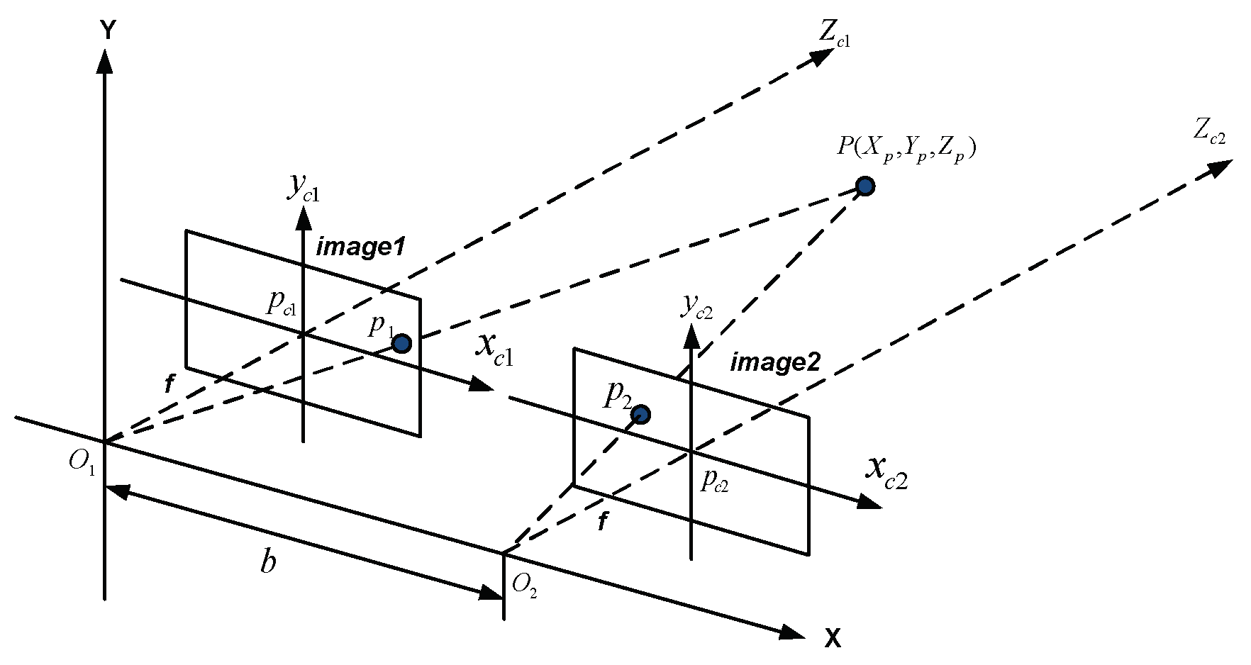
The stereo vision-based object manipulation system includes four tasks, stereo camera calibration, object feature extraction, pose estimation, and eye-to-hand calibration using adaptive network-based fuzzy inference system (ANFIS). The configuration scheme of the stereo vision is shown in Figure 1 [24]. This consists of two cameras with the same parameters to be obtained by stereo camera calibration in MATLAB [1]. Given a reference point $P(X_p,Y_p,Z_p)$, the projections in image plan 1 is $p_1(x_1,y_1)$ and in image plan 2 is $p_2(x_2,y_2)$, where f is the focal length; $d=x_1+x_2$ is the parallax; and b is the distance of two camera’s optical centers [25]. Referring to Figure 2 and the principle of similar triangles, we can get the depth Z and the X and Y coordinates of point P from Equations (1) to (3), respectively:

$$Z=b*f/d$$

(1)

$$X=Z*x_1/f$$

(2)

$$Y=Z*y_1/f$$

(3)

Before estimating the actual object distances, camera calibration is essential for determining the intrinsic and extrinsic camera parameters in computer vision tasks. (α, β, γ, u₀, v₀) stand for the intrinsic parameters, where an image plane includes u and v axes; (u₀, v₀) are the coordinates of the principal point; α and β are the axial scale factors; and γ is the parameter describing the skewness. (R, t) represent the extrinsic parameters, meaning the rotation and translation of the right camera with respect to (w.r.t.) the left camera, respectively [26].

The coordinate frame systems of the stereo vision-based object manipulation system and their relationships (${}^B\xi _E$: end-effector coordinate frame w.r.t. robot base frame, ${}^E\xi _G$: gripper to end-effector, ${}^C\xi _T$: targeted object to camera, and ${}^B\xi _T$: targeted object to robot base) are depicted in Figure 3 [24]. ${}^B\xi _C$ is the camera coordinate w.r.t. robot base that will be obtained using ANFIS so that the targeted object to robot base ${}^B\xi _T$ can be found based on the information of ${}^C\xi _T$, as shown in Figure 4.

The ANFIS architecture consists of a fuzzy layer, product layer, normalized layer, de-fuzzy layer, and summation layer. Figure 5 [24] shows the structure of a two-input type-3 ANFIS with Takagi-Sugeno if-then rule [3] as follows, in which the circle and square respectively indicate a fixed node and an adjustable node,

$$\mathrm{IF}\mathrm{x}\mathrm{is}{A}_i\mathrm{and}\mathrm{y}\mathrm{is}{B}_i\mathrm{and}\mathrm{z}\mathrm{is}{C}_i\mathrm{THEN}{Z}_i=Z_i+p_{i}x+q_{i}y+r_{i}z+s_i$$

(4)

where x and y stand for input variables; $A_i$ and $B_i$ (I = 1,2) are linguistic variables that cover the input variable universe of discourse; $z_i(x,y)(i=1:4)$ mean output variables; and $p_i,q_i$ and $r_i$ (I = 1:4) are linear consequent parameters. The layers and their functions can be described as follows:

Layer 1: Fuzzification Layer

The fuzzification is realized by the corresponding membership function, denoted by the node. The membership functions generally include adjustable parameters to provide adaptation. The Gaussian membership functions (MFs) of fuzzy sets $A_i$ and $B_i$, (i = 1, 2), ${\mu }_{Ai\left(x\right)}$, ${\mu }_{Bi\left(y\right)}$, and ${\mu }_{Ci\left(z\right)}$, are considered here and shown in Equation (5),

$$gaussmf(x,c_i,s_i)=e^{-\frac{{(x-c_i)}^2}{2s_i{}^2}}$$

(5)

where x is the input, and $c_i$ and $s_i$ are the center and standard deviation that change the shape of the MF.

Layer 2: Product Layer

The T-norm operation is used to calculate the firing strength of a rule via multiplication:

$${\omega }_i={\mu }_{Ai\left(x\right)}{\mu }_{Bi\left(y\right)}{\mu }_{Ci\left(z\right)}.$$

(6)

Layer 3: Normalization Layer

The ratio of a rule’s firing strength to the total of all firing strengths is calculated via:

$$\overline{{\omega }_i}=\frac{{\omega }_i}{{{\displaystyle \sum }}_{i=1}^6{\omega }_i}=\frac{{\omega }_i}{{\omega }_1+{\omega }_2+{\omega }_3+{\omega }_4+{\omega }_5+{\omega }_6}.$$

(7)

Layer 4: Defuzzification Layer

The linear compound is obtained from the inputs of the system as THEN part of fuzzy rules as:

$$\overline{{\omega }_i}{Z}_i\left(x,y,z\right)=\overline{{\omega }_i}\left(p_{i}x+q_{i}y+r_{i}z+s_i\right)$$

(8)

where ${\varpi }_i$ is the output of layer 3 and $\left\{p_{i}x+q_{i}y+r_{i}z+s_i\right\}$ is the consequent parameter set.

Layer 5: Summation Layer

A fixed node calculates the overall output as the summation of all incoming inputs:

$$Z= {\displaystyle \sum }_{i=1}^6\overline{{\omega }_i}{Z}_i\left(x,y,z\right)=\frac{{\omega }_1{Z}_1+{\omega }_2{Z}_2+{\omega }_3{Z}_3+{\omega }_4{Z}_4+{\omega }_5\omega Z_5+{\omega }_6{Z}_6}{{\omega }_1+{\omega }_2+{\omega }_3+{\omega }_4+{\omega }_5+{\omega }_6}.$$

(9)

The ANFIS block shown in Figure 4 consists of the inputs of ${}^C\xi _T$ or $(X_c,Y_c,Z_c,O_c)$ which are the orientation and coordinates of the targeted object base w.r.t. the camera coordinate frame, which is found by the stereo vision system for computing the solution of camera to robot arm calibration, and the outputs of ${}^B\xi _T$ or $(X_r,Y_r,Z_r,O_r)$, which are the orientation and coordinates of the targeted object w.r.t. the robot base, which is acquired by positioning the end-effector to the desired object position using the teaching box of the robot arm controller. In addition, ${}^B\xi _C$ is the camera coordinate w.r.t. the robot base that will be obtained by training the ANFIS.

3. Regions with Convolutional Neural Network (R-CNN)

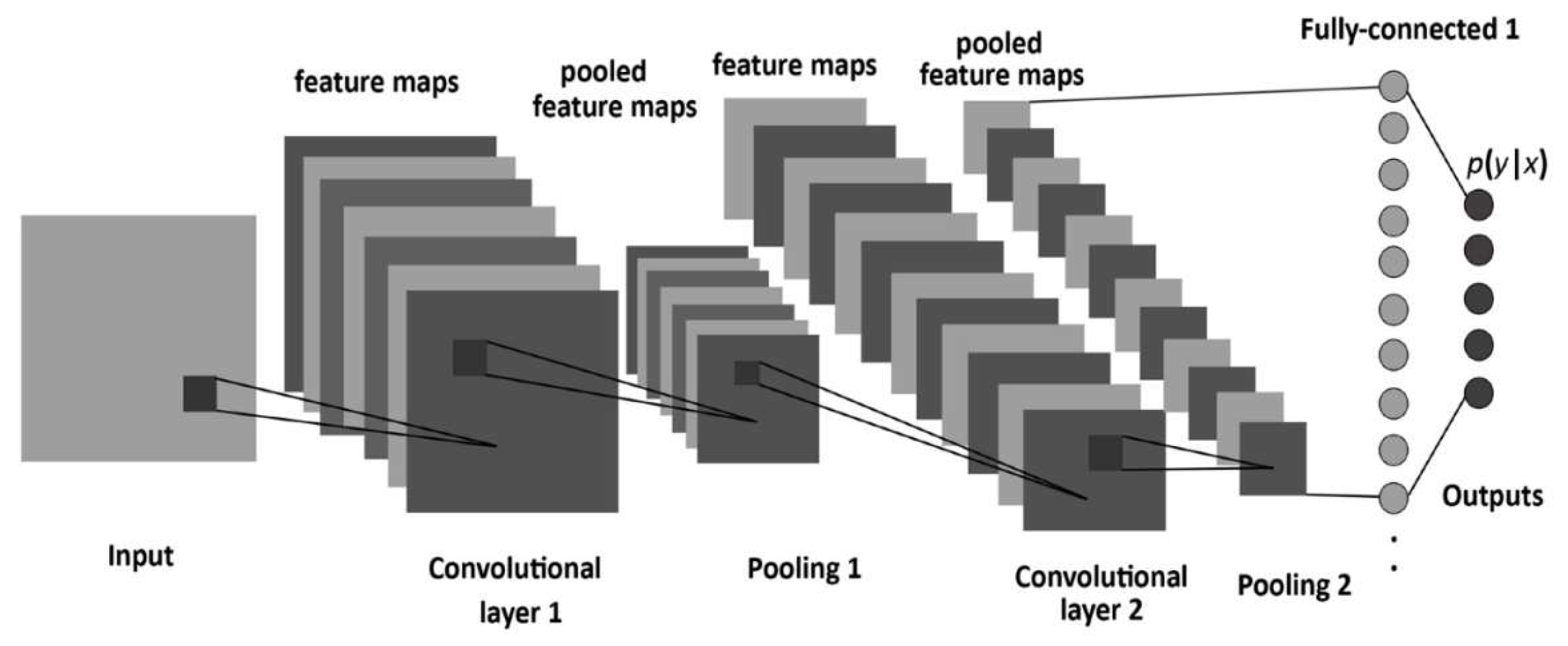
The CNN is a special class of neural networks that is best suited for the intelligent processing of visual data. It is a variation of the architecture of a multilayer neural network and is generally composed of many neural layers, including a convolutional layer, pooling layer, fully connected layer, and output layer, as shown in Figure 6 [27]. On identifying the object from a picture and marking the location, the easiest way is to use the concept of sliding a window, which is a fixed-size frame, sweeping the entire picture one by one. The output is dropped into the CNN each time to determine the classes. However, the number and size of objects to be identified are unpredictable. In order to maintain high spatial resolution, the CNN usually has two or more convolutional layers and pooling layers, which possess huge data at each layer input and result in computational complexity during processing.

A convolutional layer has a set of matrix filters that are applied to images and isolate a feature. A combination of several of these layers will build up new signs for the previous ones with signs of a lower order. In practice, this means that the network is trained to see complex features, which is a composition of simpler ones. In the process, the rectified linear unit (ReLU) is used to remove negative values for a sharper object shape. The sub-sample layer represents a layer without training, where the images are filtered with the highest value of the pixel in the window and the others ignore it. Thus, the image decreases in size and only the most significant features are left, regardless of the location. The last layer is a fully connected network, where each neuron takes in the inputs from all the outputs of the neurons of the previous layer. The obtained feature map is reduced by pooling to reduce the size of the data. The most commonly used method is max pooling. During the pooling process, there is no impact on the image, and it has a good anti-aliasing function. Before entering the fully connected layer, it is necessary to flatten it and turn the data into a straight line.

The method of region identification of regions with CNN (R-CNN) [15] is used to solve the above-mentioned problem of CNN. The image segmentation method [16] is used for selective search [17] on the input image. Then, about 2000 region proposals are selected and act as the inputs to convolutional neural networks to extract features and distinguish the regions. In this paper, in principle, we do something similar to [16] and [17], which conduct segmentation to find the centroid (XY coordinate) of an object. However, as an additional proposal in this paper, R-CNN is used to distinguish the triangle and square blocks captured from the stereo camera. Finally, the regression is used to correct the position of the frame.

An image is formed by interconnecting pixels. The pixels are also called vertices (V). The lines connecting pixels are called edges (E). Let G = (V, E) be an undirected graph with vertices $v_i\in V$, and edges $\left(v_i,v_j\right)\in \mathrm{E}$ corresponding to adjacent vertices, each having a weight $\mathrm{w}\left(v_i,v_j\right)$. There are paths at any two vertices in the graph, but those without loops are called trees. The tree with the smallest sum of the edges’ weights is called the minimum spanning tree (MST). The image segmentation method initializes each pixel as an independent vertex at the initialization time, and uses Equation (10) to calculate the similarity between each pixel,

$$pixel distance=\sqrt{{\left(r_1-r_2\right)}^2+{\left(g_1-g_2\right)}^2+{\left(b_1-b_2\right)}^2}$$

(10)

where $r_i$, $g_i$, and $b_i$ are the three color values of the pixel, respectively. To identify the similarity between two regions or a region and a pixel, a threshold is set to consider the similarity between two parts. Below the threshold, the two regions are merged into one region; thus, the threshold needs to be changed in accordance to different areas. The intra-class variation of Equation (11) is used to find the largest dissimilarity in the MST, which is also the largest luminance difference in a region,

$$Int\left(V\right)=\max w\left(v_i,v_j\right).$$

(11)

The inter-class difference method of Equation (12) will obtain the dissimilarity of the edges with the least dissimilarity between the two regions, that is, the most similar in the two regions,

$$Diff\left(V_1,V_2\right)=\min w\left(v_i,v_j\right).$$

(12)

$Int\left(V_1\right)$ and $Int\left(V_2\right)$ are the maximum differences that can be accepted by the regions $V_1$ and $V_2$, respectively, and they are larger than or equal to $Diff\left(V_1,V_2\right)$. When both regions can meet the requirements, they are merged into one region. Otherwise, they cannot be merged. Finally, using the above method, the original image can be divided into different color regions for segmentation.

The selective search first uses image segmentation to get the color regions $R=\left\{r_1,\dots ,r_n\right\}$ in the image; then, it calculates the similarity $s\left(r_i,r_j\right)$ of each adjacent region and merges the two regions with the highest degree each time. The entire image is finally merged into a few regions. The algorithm for the similarity of each region may be based on color, texture, size, and fit.

On the training data, we mark the target regions and use the labeled regions as positive samples. A selective search is used to generate the hypothetical region of the target. The region with the overlap degree between 20% and 50% of the target label region is marked as a negative sample. Then, the extracted feature is input for training. The false positive is added to the training samples to increase the number of difficult samples after each training finishes. Then, training is conducted again until convergence happens.

As for verifying, Precision (Equation (13)), Recall (Equation (14)), and Accuracy (Equation (15)) are used to describe the performance [26], where TP denotes the number of true positives, FP denotes the number of false positives, FN denotes the number of false negatives, and TN indicates the correct rejection of results (triangle or square), respectively [28],

$$Precision= \frac{TP}{TP+FP}$$

(13)

$$Recall= \frac{TP}{TP+FN}$$

(14)

$$Accuracy= \frac{TP+TN}{TP+TN+FP+FN}.$$

(15)

Hence, the disparity between our previous research [24] and the current one is that we include R-CNN to recognize objects. If the object is identified successfully, the gripper will grasp; see

Table 1. Comparison of previous with the proposed method. 6-DOF: six degrees of freedom, ANFIS: adaptive network-based fuzzy inference system, R-CNN: regions with convolutional neural network.

	Previous Method [24]	Proposed Method
Arm robotic control	inverse kinematic-6 DOF	inverse kinematic-6 DOF
Vision structure	eye to hand (stereo camera)	eye to hand (stereo camera)
Pose estimation	ANFIS	ANFIS
Centroid detection	HSV masking	image boundary
Object recognition	image segmenting	R-CNN
Object characteristic	cylindrical with some colors	triangle and square (same color)

.

4. Experimental Results

We conducted experiments to validate the proposed method. The experimental setup is shown in Figure 7, which includes a set of stereo cameras consisting of two identical Logitech C310 cameras and the targets placed anywhere in the work area. On the other hand, the robotic arm controller uses the built-in software development commands of MATLAB to drive the robotic arm through a serial communication interface and implement the proposed method through a graphical user interface (GUI). We estimated the pose of the object by using a calibrated stereo vision system and its coordinates relative to the base frame of the robot. Then, a target grabbing task is performed using a three-finger gripper and a 6-degree-of-freedom (6-DOF) robot to confirm the performance of the 3D target pose estimation in the robotic coordinate system.

According to the experimental results, the calibration of the stereo camera is successful and the internal and external parameters can be used for the triangulation process. The intrinsic and extrinsic camera parameters are first computed by stereo camera calibration, and then eye-to-eye calibration is performed. In this paper, the method proposed in [2] and the classic black-and-white checkerboard is used to calibrate a stereo camera system, which was built with two cameras with a baseline of 92 mm. The checkerboard has 63 square blocks (9 × 7 patterns) whose dimensions are 40 mm × 40 mm. For the calibration process, each camera captures 16 different positions and orientations of the 640 × 480 pixels image of the board and loads them into MATLAB. The corners of the checkerboard are detected by sub-pixel precision as input to the calibration method. The outputs include the internal matrix and the outer matrix of the two cameras and perspective transformation matrix. All of them are required to re-project the depth data to the real-world coordinates. Camera calibration is an essential part of robotic vision, but it is only a portion of this study. On the other hand, calibration is necessary to reset the camera back into its standard conditions (α, β, γ, u₀, v₀, R, t). Thus, the right and left camera are valid in estimating the position of $X_t{Y}_t{Z}_t$(target world). In the end, the pose estimation of the left camera, the pose estimation of the right camera, and the target world dataset will be compared and triangulated as $X_r{Y}_r{Z}_r$(robot world). To make sure the stereo camera is working validly, we include the stereo camera parameters in each, taking a picture. In other words, we do not use autofocus when snapping targets.

Figure 8 illustrates the difference in orientation (angle), which in this paper is known by calculating a number of the major ellipse axis to the x-axis. After calibrating the stereo camera, we take pictures from different angles to identify the target object as shown in Figure 9 and use the built-in Image Labeler of MATLAB to capture the region of interest (ROI), in which the object will be identified. As shown in Figure 10, the R-CNN is used to distinguish objects to be grasped, which are a triangle or square. After the training by R-CNN is completed, it can be tested to recognize at any position or at different angles of the object and the possibility of the targeted object (confidence). In terms of the level of confidence in our study, we set a minimum limit of 80%. If the detection results are less than that value, then the target will not be held by the gripper.

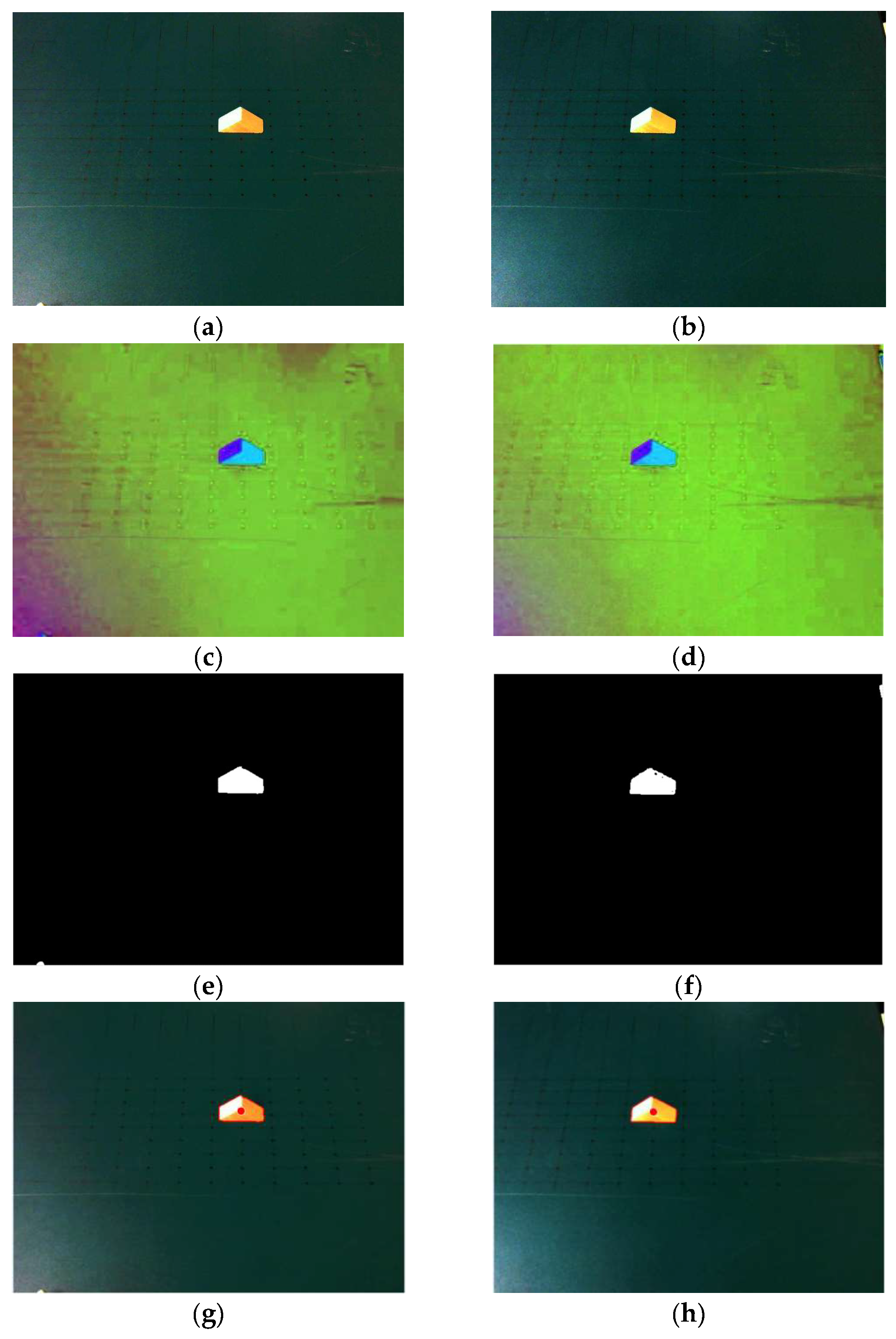
After calibrating the internal and external camera parameters of the stereo camera, the image processing system will perform the tasks of feature extraction and pose estimation. Figure 11 shows estimations of postures at each step of the target feature extraction in the two cameras. First, two cameras capture the image pair at the same time, and, based on the color, the HSV (Hue, Saturation, Value) space threshold is used to extract the target from the image and locate the boundary. Next, the boundary target and the centroid of the positioned target in the image pair are searched. Finally, the position of the target object will be determined based on the estimated centroid.

The ANFIS structure of the first-order Sugeno fuzzy system is used to perform eye-to-hand calibration training, and three, five, and seven Gaussian membership functions are respectively used to calibrate the position of the stereo camera relative to the robot arm. The centroid point of the three-dimensional object is calculated by the stereo vision system and input into ANFIS for training.

After the training process is finished, the ANFIS will learn the input and output mapping and test it with different test data.

Table 2. ANFIS training error.

No. of Input Data	No. of MFs	Training Error (mm)			Average Error (mm)
		X	Y	Z
81	3	0.086907	0.08204	0.029948	0.066298
	5	0.002016	0.002831	0.002224	0.002357
	7	0.014919	0.015392	0.013941	0.014751

shows the comparison of details and errors between different MF training results. It is found that the training error results obtained using the five membership functions were the smallest compared to the other cases. Figure 12 shows that the training error of the orientation data is 0.28923 and is reached in approximately 7000 epochs during ANFIS training. This value indicates that the target direction can be estimated with the ANFIS structure.

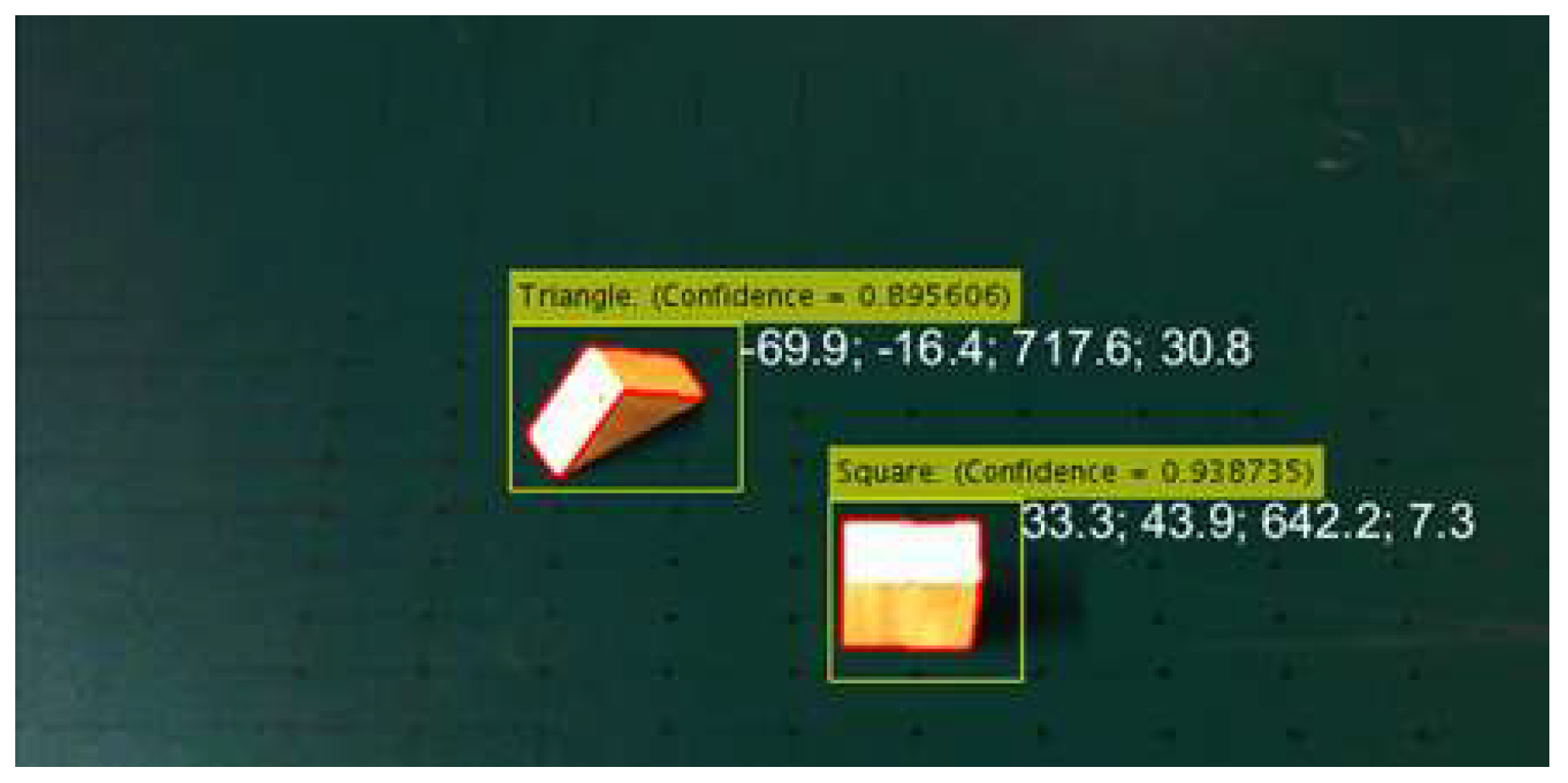
The target object identification and pose estimation experiments are conducted to validate the system performance and its orientation in the camera coordinate system, as shown in Figure 13 and Figure 14. Figure 13 shows the object name, location, and the direction estimates, that is, triangle (object name), 38.9 mm (x axis), 37.1 mm (y axis), 686.5 mm (z axis), −2.8° (orientation). Since the x, y, and z coordinates are known, then with inverse kinematics, these three points are enough to be transformed into six movements at each joint of the 6-DOF manipulators. Two different objects at any position and orientation within the workspace of the camera coordinate system have been successfully identified and detected in Figure 14. A triangular object was detected at −69.9 mm (x axis), −16.4 mm (y axis), 717.6 mm (z axis), and 30.8° (orientation), and a square object (blocks) was detected at 33.3 mm (x axis), 43.9 mm (y axis), 642.2 mm (z axis), and 7.3° (orientation). Then, the tasks of target grabbing, picking, and placing are shown in Figure 15.

Table 3. Test results of object position and orientation.

No.	Actual Coordinates and Orientation				Measured Coordinates and Orientation				Absolute Orientation Error (°)	Absolute Averaged Position Error (mm)
	X	Y	Z	Or	X	Y	Z	Or
1	267.91	327.52	289.49	−83.71	264.83	325.45	289.49	−85.85	2.14	2.575
2	106.12	345.96	294.68	−119.95	108.32	347.74	294.68	−117	2.95	1.99
3	210	360.59	287.75	−93	209.33	360.59	287.75	−93.78	0.78	0.335
4	213.52	367.92	280.85	−6	210.04	368.09	280.85	−6.23	0.23	1.655

shows the actual values and measured values for four different cases. The absolute error of the orientation and averaged absolute position error are also included. The results demonstrated that the gripper can successfully reach the target object according to the measurements of the position and orientation of the object. The manipulation system shows good performance of the 3D object pose estimation and grabbing in applications. The corresponding GUI user interface is shown in Figure 16.

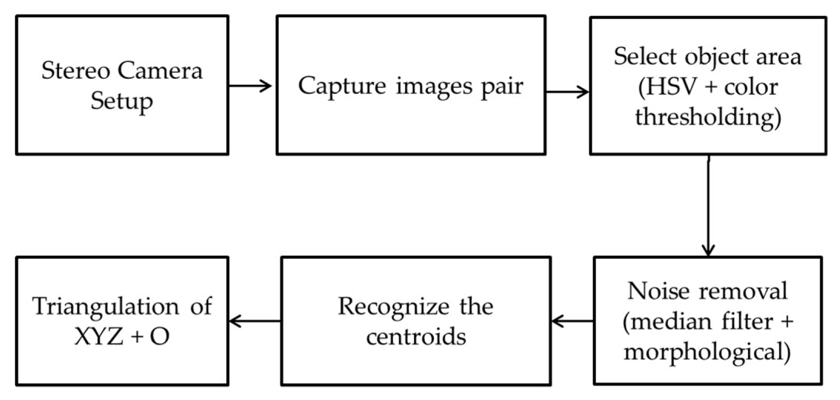
After determining the scope of the work area, image processing techniques will be used to distinguish all the objects in the range and the background. The coordinates of the camera relative to the object are obtained by triangulation. The names of all the objects in the range can be known through the use of R-CNN. ANFIS will convert the camera coordinates to the coordinates of the robotic arm. Figure 17 shows the sequence in estimating the position of XYZ + O. In the beginning, we called the stereo camera parameters from the camera calibration results. It is followed by the stereo camera taking pictures for both the right and left cameras. The second result of the image is processed to determine the object area using HSV and color thresholding. Since some color thresholding results sometimes omit the noise especially when lighting is feeble, noise removal is necessary by a median filter and a morphological filter. When the two images are completely clear from noise, using the centroid feature in MATLAB, the center of the object can be seen from two perspectives (right and left cameras). As a result, the two centroid points are triangulated with the dataset to estimate the actual position, see Figure 11g–h. Finally, the arm is driven to pick up the object and place it in a preset style and position, as shown in Figure 18, Figure 19 and Figure 20.

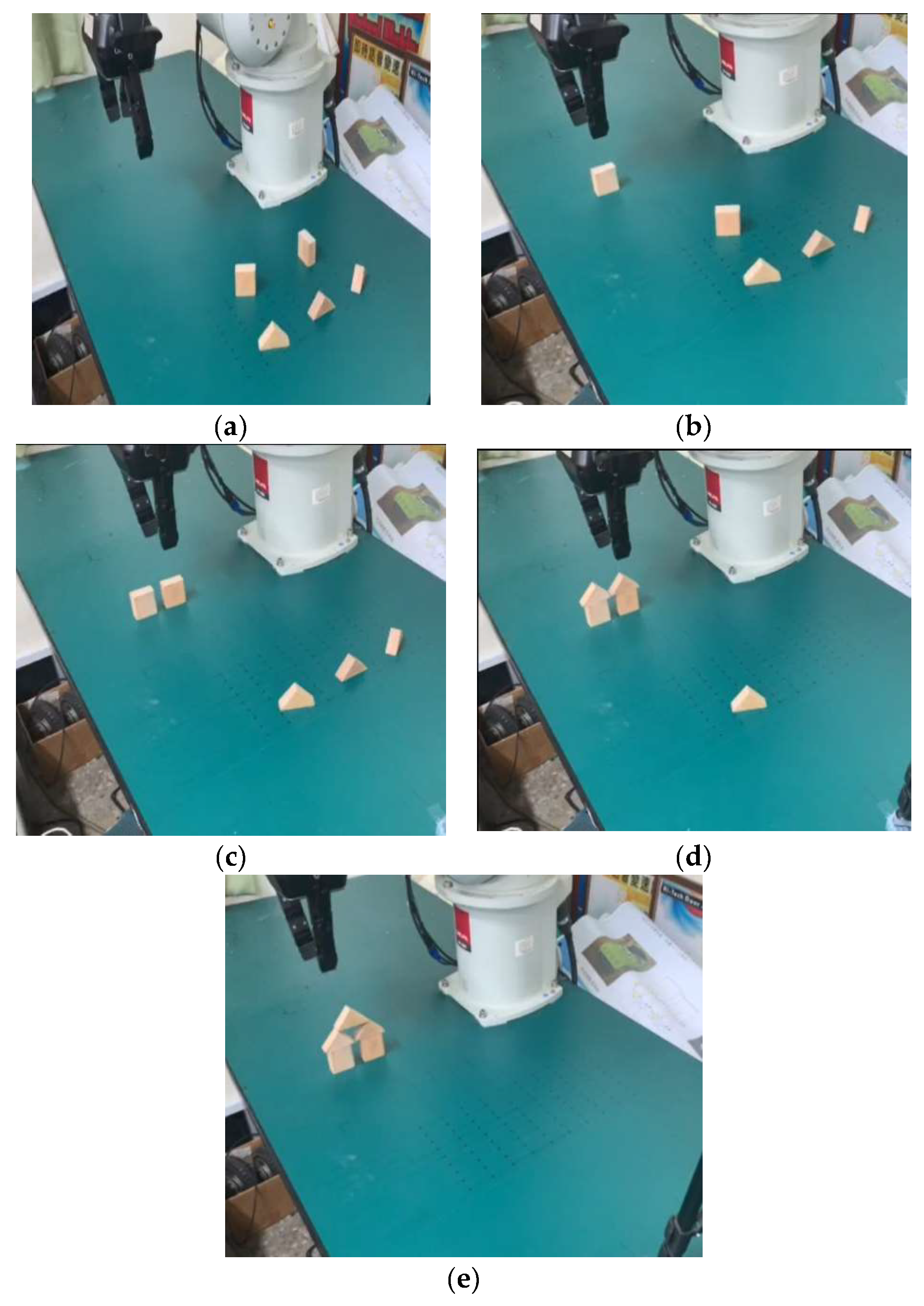
The number of datasets in the R-CNN training was 120 images and 64 images for testing. The performance of our method is very reliable that it is capable of recognizing triangles at 100% for precision, recall, and accuracy, as listed in

Table 4. Performance of R-CNN to recognize triangle and square block.

	Triangle	Square
Precision (%)	100	96.68
Recall (%)	100	100
Accuracy (%)	100	98.44

. The tendency for our method to recognize objects is only with one bounding box result. If there are many bounding boxes, then the decision to make blocks will be based on the most significant coordinate position. Examples such as Figure 18b were a square block (15.1, 61.6, 634.9, 3.0) and triangle (−99.8, −15.7, 724.2, 21.7); then, the rectangle will be grasped first by the gripper. Meanwhile, to prove the absolute errors of the estimated position and orientation, our system is tested with a scenario of setting up buildings from blocks. As shown in Figure 19, the robot arm can execute commands based on ANFIS estimation results captured from a stereo camera. In a piling position, if the error is high, it is impossible to complete the final layout such as a house.

5. Conclusions

In this paper, the coordinate frame systems of the stereo vision-based object manipulation system and their relationships are first introduced. The camera coordinate with respect to the robot base is obtained using ANFIS so that the targeted object to robot base can be easily found based on the information of the targeted object to the camera. The ANFIS architecture consists of a fuzzy layer, product layer, normalized layer, de-fuzzy layer, and summation layer, wherein the two-input type-3 first-order Sugeno fuzzy system is used to perform eye-to-hand calibration training, and three, five, and seven Gaussian membership functions are respectively used to calibrate the position of the stereo camera relative to the robot arm. From the training data, it can find that the errors are small, as shown in Table 2 and Figure 12. Based from the above results and the operation of R-CNN in the three experiments of picking and placing various numbers of blocks for specified styles and positions shown in Figure 18, Figure 19 and Figure 20, the ability of XYZ coordinate estimation with the highest error at 2575 mm can be seen. Subsequently, for orientation of 2.14 degrees, this condition is still at an acceptable level because the system is able to form a construction, as proven in Figure 19 and Figure 20. The application of R-CNN to recognize triangle blocks has precision, recall, and accuracy of 100% each. Meanwhile, percentages to identify square blocks are slightly lower, the precision is 96.88%, the recall is 100%, and the accuracy is 98.44%. Based on the testing results, we conclude the effectiveness of the proposed system.

References

- Bouguet, J.-Y. Matlab Camera Calibration Toolbox. Available online: http://www.vision.caltech.edu/bouguetj/calib_doc (accessed on 10 July 2019).
- Borangiu, T.; Dumitrache, A. Robot Arms with 3D Vision Capabilities; Intech Open Access Publisher: Rijeka, Croatia, 2010. [Google Scholar]
- Jang, J.-S.R. ANFIS: Adaptive-network-based fuzzy inference system. IEEE Trans. Syst. Man Cybern. 1993, 23, 665–685. [Google Scholar] [CrossRef]
- Tsai, R.Y.; Lenz, R.K. A new technique for fully autonomous and efficient 3D robotics hand/eye calibration. IEEE Trans. Robot. Autom. 1989, 5, 345–358. [Google Scholar] [CrossRef] [Green Version]
- Abe, S. Neural Networks and Fuzzy Systems: Theory and Applications; Springer Science & Business Media: New York, NY, USA, 2012. [Google Scholar]
- Kucuk, S.; Bingul, Z. Robot kinematics: Forward and inverse kinematics; Intech Open Access Publisher: Rijeka, Croatia, 2006. [Google Scholar]
- Mitsubishi, I.R. CRnQ/CRnD Controller Instruction Manual Detailed Explanations of Functions and Operations; The University of Tokyo: Tokyo, Japan, 2010. [Google Scholar]
- Buragohain, M.; Mahanta, C. A novel approach for ANFIS modeling based on full factorial design. Appl. Soft Comput. 2008, 8, 609–625. [Google Scholar] [CrossRef]
- Zhang, Z. A flexible new technique for camera calibration. IEEE Trans. Pattern Anal. Mach. Intell. 2000, 22, 1330–1334. [Google Scholar] [CrossRef] [Green Version]
- Maji, S.; Malik, J. Object detection using a max-margin hough transform. In Proceedings of the 2009 IEEE Conference on Computer Vision and Pattern Recognition (CVPR), Miami, FL, USA, 20–25 June 2009. [Google Scholar]
- Lecun, Y.; Bottou, L.; Bengio, Y.; Haffner, P. Gradient-based learning applied to document recognition. Proc. IEEE 1998, 86, 2278–2324. [Google Scholar] [CrossRef] [Green Version]
- LeCun, Y.; Kavukcuoglu, K.; Farabet, C. Convolutional networks and applications in vision. In Proceedings of the 2010 IEEE International Symposium on Circuits and Systems (ISCAS), Paris, France, 30 May–2 June 2010; pp. 253–256. [Google Scholar]
- Krizhevsky, A.; Sutskever, I.; Hinton, G.E. Imagenet classification with deep convolutional neural networks. Adv. Neural Inf. Process. Syst. 2012, 2012, 1097–1105. [Google Scholar] [CrossRef]
- Girshick, R.; Donahue, J.; Darrell, T.; Malik, J. Region-Based Convolutional Networks for Accurate Object Detection and Segmentation. IEEE Trans. Pattern Anal. Mach. Intell. 2016, 38, 142–158. [Google Scholar] [CrossRef] [PubMed]
- Gu, C.; Lim, J.J.; Arbel´aez, P.; Malik, J. Recognition using Regions. In Proceedings of the 2009 IEEE Conference on Computer Vision and Pattern Recognition, Miami, FL, USA, 20–25 June 2009; pp. 1030–1037. [Google Scholar]
- Felzenszwalb, P.F.; Huttenlocher, D.P. Efficient Graph-Based Image Segmentation. Int. J. Comput. Vis. 2004, 59, 167. [Google Scholar] [CrossRef]
- Sande, K.E.A.; van de Uijlings, J.R.R.; Gevers, T.; Smeulders, A.W.M. Segmentation as selective search for object recognition. In Proceedings of the 2011 International Conference on Computer Vision, Barcelona, Spain, 6–13 November 2011; pp. 1879–1886. [Google Scholar]
- Chen, Y.; Ma, Y.; Kim, D.H.; Park, S.-K. Region-Based Object Recognition by Color Segmentation Using a Simplified PCNN. IEEE Trans. Neural Netw. Learn. Syst. 2015, 26, 1682–1697. [Google Scholar] [CrossRef] [PubMed]
- Ren, Z.; Gao, S.; Chia, L.-T.; Tsang, I.W.-H. Region-Based Saliency Detection and Its Application in Object Recognition. IEEE Trans. Circuits Syst. Video Technol. 2014, 24, 769–779. [Google Scholar] [CrossRef]
- Cai, D.; Sun, X.; Zhou, N.; Han, X.; Yao, J. Efficient Mitosis Detection in Breast Cancer Histology Images by RCNN. In Proceedings of the 2019 IEEE 16th International Symposium on Biomedical Imaging (ISBI 2019), Venice, Italy, 8–11 April 2019; pp. 919–922. [Google Scholar]
- Murugan, V.; Vijaykumar, V.R.; Nidhila, A. A Deep Learning RCNN Approach for Vehicle Recognition in Traffic Surveillance System. In Proceedings of the 2019 International Conference on Communication and Signal Processing (ICCSP), India, 4–6 April 2019; pp. 157–160. [Google Scholar]
- Shi, J.; Zhou, Y.; Xia, W.; Zhang, Q. Target Detection Based on Improved Mask Rcnn in Service Robot. In Proceedings of the 2019 Chinese Control Conference (CCC), Guangzhou, China, 27–30 July 2019; pp. 8519–8524. [Google Scholar]
- He, P.; Zuo, L.; Zhang, C.; Zhang, Z. A Value Recognition Algorithm for Pointer Meter Based on Improved Mask-RCNN. In Proceedings of the 2019 9th International Conference on Information Science and Technology (ICIST), Hulunbuir, China, 2–5 August 2019; pp. 108–113. [Google Scholar]
- Taryudi; Wang, M.-S. Eye to Hand Calibration Using ANFIS for Stereo Vision-Based Object Manipulation System. Microsyst. Technol. 2018, 24, 305–317. [Google Scholar] [CrossRef]
- Liu, Z.; Chen, T. Distance Measurement System Based on Binocular Stereo Vision. In Proceedings of the 2009 International Joint Conference Artificial Intelligence (JCAI), Hainan Island, China, 25–26 April 2009; pp. 456–459. [Google Scholar]
- Zhang, Z.; Matsushita, Y.; Ma, Y. Camera calibration with lens distortion from low-rank textures. In Proceedings of the 2011 IEEE Conference on Computer Vision and Pattern Recognition (CVPR), Providence, RI, USA, 20–25 June 2011; pp. 2321–2328. [Google Scholar]
- Szegedy, C.; Liu, W.; Jia, Y. Going deeper with convolutions. In Proceedings of the IEEE Conference on Computer Vision and Pattern Recognition (CVPR ’15), Boston, Mass, USA, 7–12 June 2015; pp. 1–9. [Google Scholar]
- Zhao, W.; Ma, W.; Jiao, L.; Chen, P.; Yang, S.; Hou, B. Multi-Scale Image Block-Level F-CNN for Remote Sensing Images Object Detection. IEEE Access 2019, 7, 43607–43621. [Google Scholar] [CrossRef]
Figure 1.
Configuration scheme of stereo vision.
Figure 2.
Triangulation scheme of stereo vision.
Figure 3.
Coordinate transformation relationship.
Figure 4.
Block of the proposed adaptive network-based fuzzy inference system (ANFIS).
Figure 5.
ANFIS structure.
Figure 6.
General configuration of a convolutional neural network (CNN).
Figure 7.
Stereo camera, robot arm, gripper, and their working space.
Figure 8.
Views from various angles of the object.
Figure 9.
Marking objects.
Figure 10.
Training results.
Figure 11.
Target feature extraction and pose estimation process: (a) Color image taken by the left camera, (b) Color image taken by the right camera, (c) Image of the left camera on the HSV space, (d) Image of the right camera on the HSV space, (e) Filtered image of the left camera, (f) Filtered image of the right camera, (g) Object pose estimation on the left camera, and (h) Object pose estimation on the right camera.
Figure 12.
Minimum training error of ANFIS in the target orientation.
Figure 13.
Object name and location and their orientation estimation results.
Figure 14.
Estimation results of two object names and positions and their orientations.
Figure 15.
Estimations of the object and the gripper (a) The measured orientation of the object is 85.85°, (b) The orientation of the gripper is 83.71°, (c) The measured orientation of the object is 117°, (d) The orientation of the gripper is 119.95°, (e) The measured orientation of the object is 93.78°, (f) The orientation of the gripper is 93°, (g) The measured orientation of the object is 6.23°, (h) The orientation of the gripper is 6°.
Figure 16.
User interface.
Figure 17.
The sequence of processes in estimating the position of XYZ + O.
Figure 18.
Operation process: (a) Get the image in the working range, (b) Image processing, (c)–(f) Pick and place objects intentionally for the first specified layout style.
Figure 19.
Operation process: (a)–(e) The second layout style.
Figure 20.
Operation process: (a)–(e) The third layout style.