Multiscale Image Matting Based Multi-Focus Image Fusion Technique

Abstract

Multi-focus image fusion is a very essential method of obtaining an all focus image from multiple source images. The fused image eliminates the out of focus regions, and the resultant image contains sharp and focused regions. A novel multiscale image fusion system based on contrast enhancement, spatial gradient information and multiscale image matting is proposed to extract the focused region information from multiple source images. In the proposed image fusion approach, the multi-focus source images are firstly refined over an image enhancement algorithm so that the intensity distribution is enhanced for superior visualization. The edge detection method based on a spatial gradient is employed for obtaining the edge information from the contrast stretched images. This improved edge information is further utilized by a multiscale window technique to produce local and global activity maps. Furthermore, a trimap and decision maps are obtained based upon the information provided by these near and far focus activity maps. Finally, the fused image is achieved by using an enhanced decision maps and fusion rule. The proposed multiscale image matting (MSIM) makes full use of the spatial consistency and the correlation among source images and, therefore, obtains superior performance at object boundaries compared to region-based methods. The achievement of the proposed method is compared with some of the latest techniques by performing qualitative and quantitative evaluation.

1. Introduction

During image acquisition, one of the most important objectives is obtaining a focused region of interest. However, because of the limited field depth, the focused region contains sharp edges, whereas the other regions get blurred. Recently, multi-focus image fusion (combine images with different focused objects) has received tremendous attention amongst the researchers. This fused image offers high quality containing more detailed information [1,2]. Several methods are developed to fuse multiple images, which are broadly grouped into transform and spatial domains [3,4].

Transform domain methods fuse the corresponding transform coefficients and employ inverse transformation to construct the fused image. Spatial domain methods are further classified into pixel [5,6] and region based methods [7,8]. The spatial domain methods form the fuse image by choosing the pixels/regions/blocks that are focused. Transform domain-based methods in dynamic scenes merge these coefficients without considering the spatial properties, resulting in artifacts in the fused image. Furthermore, pixel and region-based methods are unable to produce the best fusion results for images with complicated texture patterns [1].

Zhang et al. [9] used morphological operations to extract focus regions. However, this technique suffers from block artifacts. De et al. [10] utilized morphological processes to detect the focused region and suggested a technique for calculating an optimized block size. The fused result still suffers from blocking effects. Later on, Bai et al. [11] presented a novel quadtree decomposition and a weighted focus based image fusion technique. However, this technique also provides inaccurate segmentation and low visual effects because of the smooth regions. Yin et al. [12] proposed a method based on joint dictionary and singular value decomposition (SVD) methods. Still, this method is not effective computationally because of the individual training for sub dictionaries and SVD computation.

Li et al. [13] explored guided filtering (GFF) and spatial information to improve the fusion results by mitigating the block effects. Zhang et al. [14] proposed a multifocus image scheme based upon a visual saliency method. Recently, image matting has been used for effectively differentiating the focused and out-of-focus regions. These methods can be broadly categorized as supervised matting and unsupervised matting techniques. Supervised methods require a user specified foreground and background regions known as trimap. Therefore, such techniques require human experts, are time consuming, and produce inconsistent results for images with high-textured backgrounds. However, unsupervised methods are better than supervised ones because user interaction is not required for achieving a good matting result. Chen et al. [15] used a parametric edge based method. However, these methods do not consider the artifacts among the smooth regions, and much of it depends on the performance of hand crafted features, which require much expert knowledge. Li et al. [16] proposed multifocus matting (MFM) based image fusion by combining together the focus region and its neighboring pixels. This method marginally improves the fusion results and also overcomes some shortcomings of spatial domain methods.

Xiao et al. [17] used depth information to segment an image into focus and blur regions. Zhang et al. [18] made use of log spectrum, Fourier transform, and Bayesian techniques. In [19], a definite focus region is detected by using a novel multi scale gradient information. Liu et al. [20] proposed a transform (which is scale invariant) to detect focus regions. However, this technique fails to offer sharp edges of the focus regions. Furthermore, in [21], the focus information was extracted by using texture features. Baohua et al. [22] performed the near and far focus region detection by using a sparse representation and guided filter techniques. In [23], a structure tensor was used for the detection of high and low frequency components. However, this technique fails to provide a visible difference between focus and defocus regions in many cases. Yu at.al. [24] presented a convolutional neural network (CNN) based multifocus image fusion technique. However, in this method, the precision of recognizing the focus block is very low.

In this paper, a novel multi-focus image fusion method is presented using contrast stretching and spatial gradients to enhance the edges from the source images. A multiscale sliding window method is used for detecting the local and global intensity variations to generate initial activity maps. These multiple activity maps are further processed to generate a trimap. An enhanced image matting technique is used for generating the decision maps. Finally, the fused image is obtained after processing the source images, enhanced decision maps, and employing the fusion rule.

2. Proposed Fusion Technique

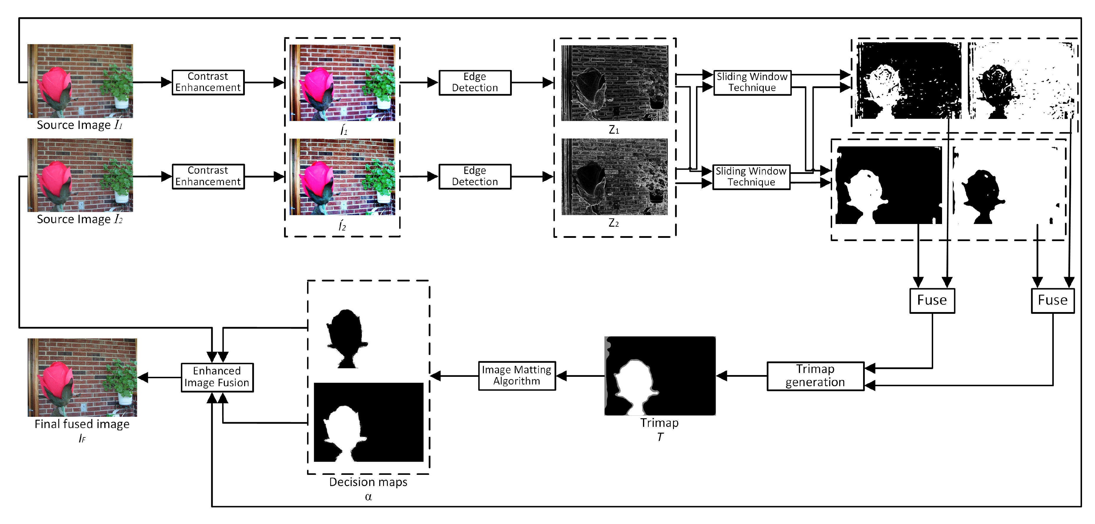
The schematic diagram of the proposed algorithm is shown in Figure 1. It can be observed that in the first step, a contrast enhancement scheme is applied on the source images. In the second step, the outcome of the intensity transformed image is processed through an edge detection method. In a multi-focus image fusion scheme, the selection of near focus and far focus region plays a vital role. The region that is in focus during image acquisition tends to have sharp edges as compared to the out-of-focus region. Therefore, these sharp edges can be detected easily by applying an appropriate edge detection method.

The edge detection schemes rely heavily on the intensity distribution of an image. A poor intensity distribution can lead to an oversaturated, undersaturated, dark, or bright image. In either of those images, the edge detection algorithm cannot perform well. In order to improve the intensity distribution of an image, an intensity transformation can be performed. In Figure 2, the improvement in edge information is shown by comparing the images before and after applying the contrast enhancement scheme. In the next step, a sliding window technique with two different scales is applied on both edges of the detected images to generate activity maps. In this step, both local and global intensity variations are analyzed. The fine details are more prominent under a small sliding window scale. These masks are further fused together and processed to generate a trimap. Next, the trimap undergoes an image matting transformation to produce refined decision maps, which produces the final fused image. The proposed fusion scheme, along with the equation references, is also elaborated in Algorithm 1.

Let $I_i$ be the source color images with $M\times N$ dimensions where, $m=1,2,\dots ,M$, $n=1,2,\dots ,N$ and $i\in [1,2]$ represents near and far focus images, respectively.

Algorithm 1: Proposed MSIM based Fusion Technique.

Require:$I_i$, $i\in [1,2]$

Step 1. Apply contrast enhancement on $I_i$ using Equation (1).

Step 2. Apply edge map on ${\stackrel{\prime }{I}}_i$ using Equation (2) to Equation (5).

Step 3. Compute activity maps, $G_{i,\sigma }^{\prime }$$\stackrel{\sigma =1}{\leftarrow }$w, $Z_i$ using Equation (6).

Step 4. Compute Smooth Activity maps, $G_{i,\sigma }$$\stackrel{\mathrm{Sum}\mathrm{Filter},\sigma =1}{\leftarrow }$$G_{i,\sigma }^{\prime }$, using Equation (7).

Step 5. Compute Score maps, ${\zeta }_{i,\sigma }$$\stackrel{\sigma =1}{\leftarrow }$$G_{i,\sigma }$, using Equations (8) and (9).

Step 6. Repeat Steps 3, 4, and 5 with $\sigma =3$.

Step 7. Compute Near focus ($D_1$) and Far focus ($D_2$) using Equation (10).

Step 8. Generate Trimap T using Equation (11).

Step 9. Generate Alpha Matte $\alpha$ using Equation (14).

Step 10. Generate Fused Image $A_F$ using Equation (15).

2.1. Contrast Enhancement

Improving the enhancement of the low contrast image, the histogram equalization seems an effective method. Non-parametric modified histogram equalization (NMHE) [25] is integrated to enhance the contrast and preserves the mean brightness of the source image $I_i$, i.e.,

$$\begin{array}{c}\stackrel{\prime }{I_i}\stackrel{\mathrm{NMHE}}{\leftarrow }{I}_i\hfill \end{array}$$

(1)

Image development in contrast centrally improves and concentrates pixel details. Figure 2 shows the enhancement in edge information. Figure 2a,b shows the far and near focus source image, respectively, and their gradients are shown in Figure 2c,d. Contrast enhanced of near and far focus images are displayed in Figure 2e,f, and their respective edge maps are shown in Figure 2g,h, respectively. From the images, it can be clearly seen that after the enhancement algorithm, the gradients of the source image were greatly improved.

2.2. Edge Detection

The edges of the images after contrast enhancement is done by a spatial stimuli sketch model (SSGSM) [26] technique, which principally focuses on focal intensity points and edges in an image, and then the unknown region is calculated in the coarse decision maps by implementing the concentrated information in both the activity level maps. The weight of the local stimuli is deliberated by detecting the local variation in the perceived brightness at the respective positions. The discerned brightness, $P_i$ of a specific image is given in Equation (2) as,

$$P_i=\vartheta {log}_{10}\left(\stackrel{\prime }{I_i}\right)$$

(2)

where, $\stackrel{\prime }{I_i}$ represents the source images, and $\vartheta$ denotes the scaling factor.

Gradients illustrate the sharp intensity variations in the image. Mathematically, the weight is computed as the total difference of the perceived brightness on x and y directions. The intensity variations of $P_i$ on the x and y axis are represented by ${\varrho }_i^x$ and ${\varrho }_i^y$, respectively. These variations are calculated by using their respective gradients $B_i^x$ and $B_i^y$, given as in Equations (3) and (4):

$$[B_i^x,B_i^y]\stackrel{\mathrm{gradient}}{\leftarrow }{P}_i$$

(3)

$${\varrho }_i^x=B_i^x(e^{-|B_i^x|});{\varrho }_i^y=B_i^y(e^{-|B_i^y|})$$

(4)

The weight of local stimuli $Z_i$ is expressed by using Equation (5):

$$Z_i=\sqrt{{\left({\varrho }_i^x\right)}^2+{\left({\varrho }_i^y\right)}^2}$$

(5)

2.3. Focus Maps

A multiscale sliding window technique is applied to acquire diverse focus maps from activity maps $Z_i$. Two sliding windows are selected for the generation of focus maps. Firstly, a $9\times 9$ window is initialized by setting $k=9$, $l=9$ and $\sigma =1$ in Equation (6). The activity maps are divided into blocks of $9\times 9$ pixels by using spatial domain filters, as in Equations (6) and (7):

$$\begin{array}{c}\hfill G_{i,\sigma }^{\prime }(m,n)=\sum _{q_1=-\sigma \times k}^{\sigma \times k}\sum _{q_2=-\sigma \times l}^{\sigma \times l}w(q_1,q_2)Z_i(m+q_1,n+q_2)\end{array}$$

(6)

$$\begin{array}{c}\hfill G_{i,\sigma }(s,t)=\sum _{(m,n)ϵ\mathsf{\Omega }}{G}_{i,\sigma }^{\prime }(m,n)\end{array}$$

(7)

The activity of each block is stored in the form of map scores. Furthermore, the sum of intensity levels in each near ($G_{1,\sigma =1}(s,t)$) and far focus block ($G_{2,\sigma =1}(s,t)$) are calculated and compared with one another to update the score maps (${\zeta }_{i,\sigma =1}$), as given in Equations (8) and (9).

$${\zeta }_{1,\sigma }(m,n)=\left\{\begin{array}{cc}1,\hfill & \mathrm{if}{G}_{1,\sigma }(s,t)>G_{2,\sigma }(s,t)\hfill \\ 0,\hfill & \mathrm{Otherwise}\hfill \end{array}\right.$$

(8)

$$\begin{array}{c}\hfill {\zeta }_{2,\sigma }(m,n)=1-{\zeta }_{1,\sigma }(m,n)\end{array}$$

(9)

Similarly, $27\times 27$ block of pixels are generated by setting $k=9$, $l=9$ and $\sigma =3$ in Equation (6). The activity maps in each near ($G_{1,\sigma =3}(s,t)$) and far focus block ($G_{2,\sigma =3}(s,t)$) are calculated and compared with one another to update the score maps (${\zeta }_{i,\sigma =3}$), as in Equations (8) and (9).

These multiple sliding windows result in multiple near and far focus maps. This multiscale sliding window technique reduces the blocking artifacts in the coarse decision maps. Each map offers different characteristic information, which plays a key role in improving the focus maps and the fused image. These multiscale windows extract the information from original images at different scales. It is noted that this approach has demonstrated better visual quality than the existing methods. Each scale offers different information for image fusion, for example, a small window size focuses on local intensity variations, whereas a large size window size extracts global variations in an image. The information from these multiscale near-focus (${\zeta }_{1,\sigma =1}$ and ${\zeta }_{1,\sigma =3}$) and far-focus maps (${\zeta }_{2,\sigma =1}$ and ${\zeta }_{2,\sigma =3}$) are combined together to form a single near-focus ($D_1$) and far-focus ($D_2$) map, respectively, carrying the attributes of both scales, as in Equation (10).

$$\begin{array}{c}\hfill D_i(m,n)\stackrel{\mathrm{AND}}{\leftarrow }{\zeta }_{i,\sigma =1},{\zeta }_{i,\sigma =3}\end{array}$$

(10)

After obtaining the focus maps, the next step is to generate a trimap that segments the given images into the three different regions, i.e., focused, definite defocused, and unknown. Pixels from the focused region have greater focus value than pixels in the defocused region [27]. The trimap T of $A_1$ is processed by using $D_1$, $D_2$ as in Equation (11).

$$\begin{array}{c}T\stackrel{\mathrm{Tri}\mathrm{Map}}{\leftarrow }{D}_i\hfill \end{array}$$

(11)

In a given image I, the image matting considers it a composite of foreground $I^{Fore}$ and background $I^{back}$. Each pixel is assumed to be a linear combination of $I^{Fore}$ and $I^{back}$. Let $\alpha$ denote the pixel foreground opacities then an image I can be represented as,

$$\begin{array}{c}\hfill I_i={\alpha }_i{I}_i^{Fore}+(1-{\alpha }_i)I_i^{back}\end{array}$$

(12)

In [28], the quadratic cost function for $\alpha$ is derived as,

$$\begin{array}{c}\hfill J\left(\alpha \right)={\alpha }^{T}L\alpha \end{array}$$

(13)

where, L is defined as a matting laplacian matrix of $N\times N$ dimension.

The L is a symmetric positive definite matrix and is defined in [28] as L = H − W, where, H is a diagonal matrix and W is a symmetric matrix. The neighborhood $W_M$ is given as,

$$\begin{array}{c}\hfill W_M(i,j)=\sum _{k/(i,j)ϵw_k=0}^K\frac{1}{|w_k|}\left(1+({\chi }_i-{\varphi }_k){({\nu }_k+\frac{\epsilon }{|w_k|}\mathsf{\Gamma })}^{-1}({\chi }_j-{\varphi }_k)\right)\end{array}$$

(14)

where, $|w_k|$ denotes the number of pixels in the window, ${\varphi }_k$ and ${\nu }_k$ represents mean and variance of intensities in the window $w_k$, respectively. $\chi$ represents the pixel color, $ϵ$ is a regularization parameter and $\mathsf{\Gamma }$ is an identity matrix.

Finally, the obtained alpha matte $\alpha$ from the source images and trimap is same as the focused region of $I_i$ is constructed as in Equation (15).

$$I_F(m,n)=\alpha (m,n)I_1(m,n)+(1-\alpha (m,n))I_2(m,n)$$

(15)

3. Results and Discussion

To show the superiority of the proposed MSIM, a comparison was performed with discrete wavelet transform (DWT) [29], guided filtering based fusion (GFF) [13], discrete cosine transform (DCT) [30], dense sift (DSIFT) [20], multi-scale morphological focus-measure (MSMFM) [9], and convolutional neural network (CNN) [24] on a multifocus image dataset [31]. The proposed method was evaluated by performing both subjective and objective assessments. These algorithms were tested on a Acer laptop Intel(R) Core™ i7 2.6GHz processor with 12GB RAM under a Matlab R2018b environment. All the algorithms were executed by using the original codes made available by the authors.

3.1. Comparison of Image Matting Result

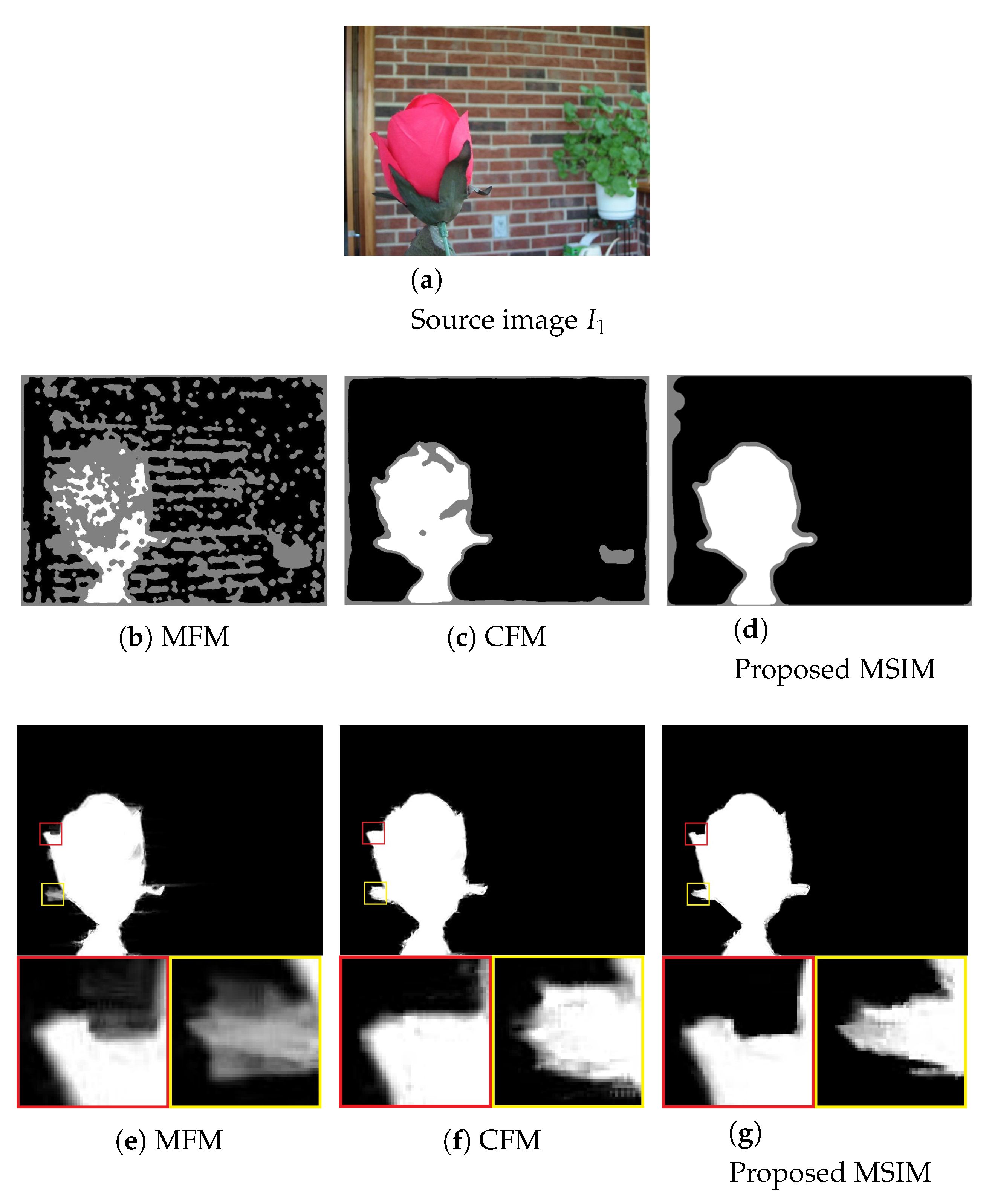
Generally, an unsupervised trimap produces better results than the supervised ones. Hence, in practice, user specified trimaps are often necessary to achieve the high quality matting results; however, the making of a user supervised trimap takes time, skills, and is not available for all kind of images. In this paper, two image matting techniques have been proposed, i.e., focus maps matting and feature based matting. The results of the proposed method are compared with feature based matting and the closed form matting [28]. It is clearly observed that the proposed matting produces better results compared to the existing technique (Figure 3).

3.2. Comparison of Image Fusion with Other Methods

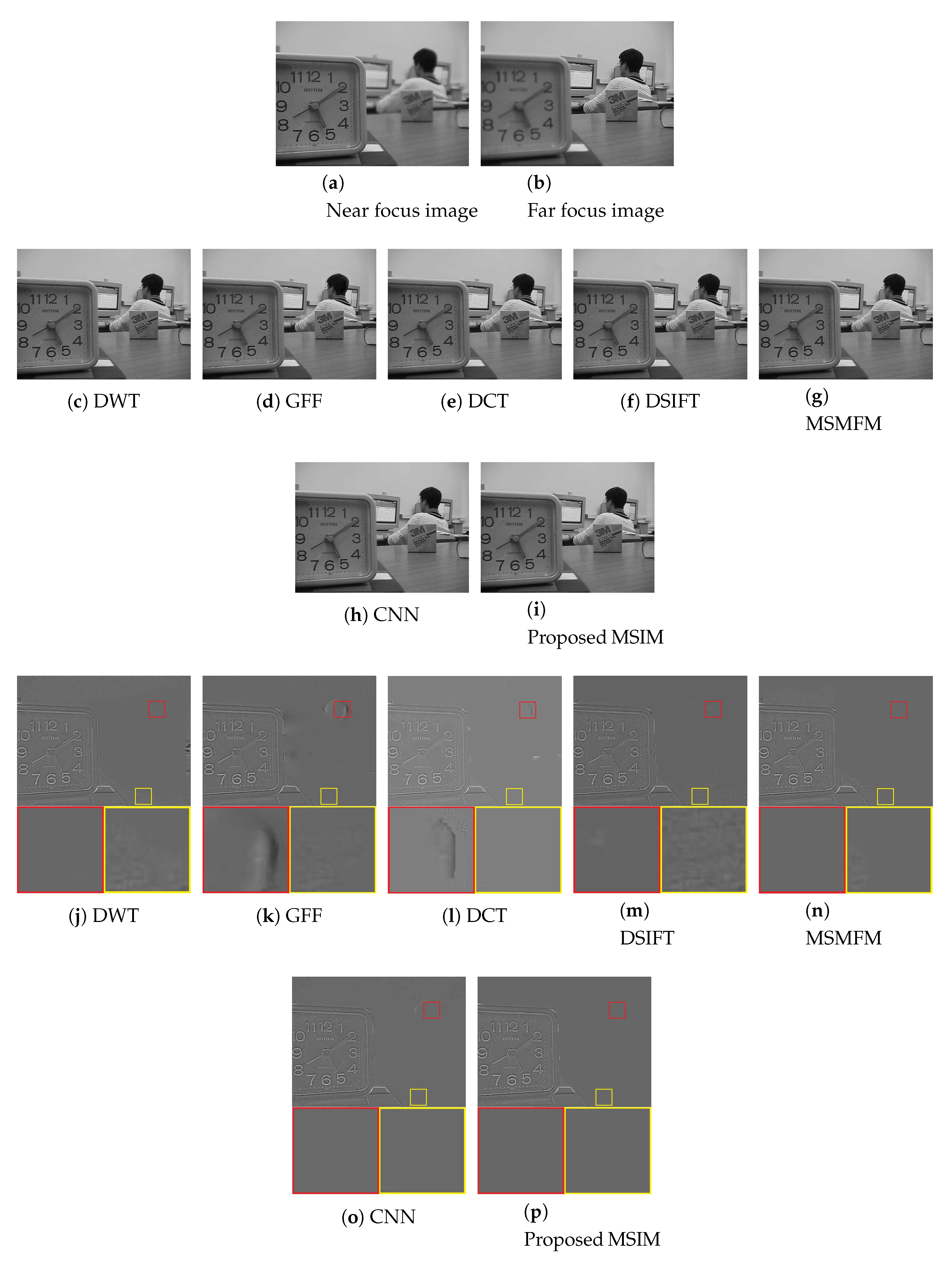
The proposed technique is tested on gray scale, color, and dynamic images. Figure 4 shows the results of the proposed MSIM for “Lab” image. The source near and far focus inputs are presented in Figure 4a,b, respectively. The fused results produced by other methods and the proposed technique are given in Figure 4c–i. To further investigate the effectiveness, the difference of the near-focus image with the fused images is shown in Figure 4j–p. The close up views enclosed by red and yellow boxes are also shown at the bottom of their respective difference image. It is noted that the DWT, DCT, and DSIFT methods produce poor edge information and contain artifacts (as shown in the close-ups). Furthermore, GFF, MSMFM, and CNN methods also provide limited information of the focused regions as compared to the proposed MSIM technique. Similarly, Figure 5 illustrates the results produced by several existing and proposed algorithms for “Globe” images. To further analyze the results, close-up views of important regions are placed at the bottom of each difference image. In this image, the boundary region of the hand is difficult to detect since it lies on the focus transition point. The results of fusion by other techniques in Figure 5j–o show the distorted regions and lack of sharpness in the highlighted region. However, the proposed MSIM method has successfully fused the complementary information from both the images, as shown in Figure 5p. It is very important to evaluate the results of different algorithms on the color dataset shown in Figure 6a,b and Figure 7a,b. The outcomes of the existing techniques and the proposed method on “Flower” and “Boy” are shown in Figure 6c–i and Figure 7c–i, respectively. The difference between the fused and out of focus source images is illustrated in Figure 6j–p and Figure 7j–p, respectively. It is noted that in both the flower and boy images, the existing techniques are unable to mitigate the artifacts and blur in the focus transition area (as noted in the close-ups of difference images). The proposed MSIM is able to preserve contrast and details using the edge feature and multi scale image matting technique.

Another challenge for multi-focus fusion includes the performance in dynamic scenes. The scenario occurs either due to the movement of the camera or the motion of the object. So it is important to verify the effectiveness of the MSIM result with the existing ones on such scenes. Figure 8a,b shows near and far focus “Girl” images, respectively. The results of MSIM and existing techniques are shown in Figure 8c–i, while Figure 8j–p shows difference images. As shown in the red and yellow boxes, the DWT, GFF, DCT, DSIFT, and MSMFM methods are unable to completely fuse the focus regions. Moreover, the CNN has produced erosion in the fused image, whereas the proposed MSIM has successfully mitigated the inconsistencies and limitations of the existing techniques.

It is observed from these visualizations that the existing methods produce artifacts, erosion, halo effects and are unable to produce sharp boundaries of the near and far focus images. Note that the MSIM technique not only perfectly identifies the near and far focus regions but also fuses the complementary information in an effective manner.

3.3. Objective Evaluation Metrics

After evaluating the visual quality and quantitative assessment of different methods, it can be clearly observed that MSIM produces a visually pleasant and high quality fusion result in almost all cases and outperformed the existing fusion methods for multi-focus images. Five most commonly used metrics are evaluated, i.e., Mutual Information (MI) [32], Spatial Structural Similarity (SSS) $Q^{AB/F}$ [33], Feature Mutual Information (FMI) [34], Entropy (EN) [35], and Visual Information Fidelity (VIF) [36] to verify the superiority and effectiveness of the proposed MSIM method.

Table 1. The quantitative assessment of different fusion methods.

Images	Fusion Methods	MI [32]	${\mathit{Q}}^{\mathbf{AB}/\mathit{F}}$ [33]	FMI [34]	EN [35]	VIF [36]	Time/s
	DWT [29]	8.2152	0.7239	0.8190	7.0474	0.9138	4.02
	GFF [13]	7.9114	0.7279	0.8191	7.0602	0.9149	3.11
	DCT [30]	8.5263	0.7460	0.9197	6.9819	0.9143	11.56
Lab	DSIFT [20]	8.5212	0.7478	0.9097	7.0759	0.9171	6.65
	MSMFM [9]	8.7995	0.6864	0.9196	6.9885	0.9161	5.79
	CNN [24]	8.6812	0.7471	0.9196	6.9974	0.9159	7.88
	Proposed	8.8322	0.7474	0.9386	7.1759	0.9980	5.08
	DWT [29]	8.1910	0.7246	0.8892	7.7037	0.9240	11.09
	GFF [13]	8.7664	0.7726	0.8935	7.7412	0.9476	9.78
	DCT [30]	9.1845	0.7731	0.8939	7.6990	0.9374	10.98
Globe	DSIFT [20]	9.1435	0.7746	0.8938	7.6989	0.9437	5.51
	MSMFM [9]	9.3739	0.7711	0.8940	7.7389	0.9439	6.55
	CNN [24]	9.2397	0.7701	0.8927	7.7458	0.9472	8.01
	Proposed	9.4316	0.7733	0.8943	7.7479	0.9480	7.06
	DWT [29]	5.6452	0.6536	0.8773	7.1701	0.9064	16.93
	GFF [13]	7.3290	0.6944	0.8908	7.1915	0.9200	10.13
	DCT [30]	7.8561	0.6785	0.8861	7.4331	0.9263	12.03
Flower	DSIFT [20]	8.0057	0.6947	0.8857	7.4316	0.9304	4.61
	MSMFM [9]	7.9233	0.6930	0.8915	7.1873	0.9140	5.98
	CNN [24]	3.0773	0.6951	0.8912	7.1872	0.9177	7.32
	Proposed	8.1458	0.7940	0.8936	7.5897	0.9367	6.91
	DWT [29]	7.5321	0.7206	0.8814	7.5371	0.8935	9.95
	GFF [13]	7.6316	0.7448	0.8717	7.5310	0.8097	5.97
	DCT [30]	8.0852	0.7409	0.8714	7.5669	0.9035	11.08
Boy	DSIFT [20]	8.1765	0.7437	0.8721	7.5388	0.9048	3.80
	MSMFM [9]	8.2081	0.7418	0.8717	7.2402	0.9026	7.55
	CNN [24]	2.9966	0.7466	0.8819	7.5386	0.9072	8.01
	Proposed	8.2961	0.7487	0.8826	7.5673	0.9077	7.75
	DWT [29]	5.6226	0.5939	0.8189	7.8477	0.6486	5.39
	GFF [13]	8.0820	0.6902	0.8213	7.8475	0.6448	5.88
	DCT [30]	8.7222	0.6788	0.8168	7.8226	0.7332	6.44
Girl	DSIFT [20]	8.8774	0.6834	0.8215	7.8429	0.7394	4.04
	MSMFM [9]	9.0368	0.5427	0.8219	7.6549	0.7397	7.11
	CNN [24]	8.8580	0.6919	0.8208	7.8607	0.7417	10.21
	Proposed	9.0970	0.6936	0.8415	7.8749	0.7468	5.65

shows that the proposed MSIM gives better objective assessment results than the existing methods. Although, the results of existing techniques are comparable in some cases (Flower and Boy); however, the metric values obtained using the proposed MSIM generally outperforms the existing techniques.

3.4. Comparison of Computational Efficiency

In this section, the computational efficiency of different fusion methods is compared. The execution time of these schemes for different images is shown in Table 1. The results show that the proposed MSIM, DSIFT, and GFF consume less time as compared to the other algorithms DCT, DWT, MSMFM, and CNN. The MSMFM algorithm uses a multi-scale morphological gradient based feature, therefore taking longer processing time than DSIFT. Whereas, GFF integrates the source images by using a global weight based scheme; however, it still takes less computation time and produces satisfactory results.

The proposed method utilizes the contrast enhancement, SSGSM based edge extraction, sliding window based local and global operations to create activity maps and trimap. The sliding window method, activity maps generation, their comparison, and a trimap generation are time consuming tasks. Although, the proposed algorithm consumes more processing time as compared to the existing ones; however, it produces the best unsupervised image matting and image fusion results.

4. Conclusions

A multiscale image fusion technique is presented for accurate construction of tri-maps, decision maps, and fused images. Firstly, the source images are pre-processed using a NMHE histogram equalization method and their gradients are computed using SSGSM. A multiscale sliding window technique calculates the focus maps from source images. Furthermore, the focus information is processed so that an accurate focused region is extracted. The proposed MSIM is robust to noise interference and is flexible to combine various fusion strategies and provides better fusion performance both visually and quantitatively when compared with other state of the art methods for multi-focus images datasets. In the future, the proposed scheme will be further considered for other application areas of image processing.

References

- Li, S.; Kang, X.; Fang, L.; Hu, J.; Yin, H. Pixel-level image fusion. A survey of the state of the art. Inf. Fus. 2017, 33, 100–112. [Google Scholar] [CrossRef]
- Maqsood, S.; Javed, U. Multi-modal Medical Image Fusion based on Two-scale Image Decomposition and Sparse Representation. Biomed. Signal Process. Control 2020, 57, 101810. [Google Scholar] [CrossRef]
- Thang, C.; Anh, D.; Khan, A.W.; Karim, P.; Sally, V. Multi-Focus Fusion Technique on Low-Cost Camera Images for Canola Phenotyping. Sensors 2018, 18, 1887. [Google Scholar]
- Goshtasby, A.A.; Nikolov, S. Image fusion: Advances in the state of the art. Inf. Fus. 2007, 8, 114–118. [Google Scholar] [CrossRef]
- Yang, Y.; Yang, M.; Huang, S.; Ding, M.; Sun, J. Robust sparse representation combined with adaptive PCNN for multifocus image fusion. IEEE Access 2018, 6, 20138–20151. [Google Scholar] [CrossRef]
- Eltoukhy, H.A.; Kavusi, S. A computationally efficient algorithm for multi-focus image reconstruction. SPIE Electr. Imaging Proc. 2003, 332–341. [Google Scholar]
- Zribi, M. Non-parametric and region-based image fusion with Bootstrap sampling. Inf. Fus. 2010, 11, 85–94. [Google Scholar] [CrossRef]
- Qilei, L.; Xiaomin, Y.; Wei, W.; Kai, L.; Gwanggil, J. Multi-Focus Image Fusion Method for Vision Sensor Systems via Dictionary Learning with Guided Filter. Sensors 2018, 18, 2143. [Google Scholar]
- Zhang, Y.; Bai, X.; Wang, T. Boundary finding based multi-focus image fusion through multi-scale morphological focus-measure. Inf. Fus. 2017, 35, 81–101. [Google Scholar] [CrossRef]
- De, I.; Chanda, B. Multi-focus image fusion using a morphology-based focus measure in a quad-tree structure. Inf. Fus. 2013, 14, 136–146. [Google Scholar] [CrossRef]
- Bai, X.; Zhang, Y.; Zhou, F.; Xue, B. Quadtree-based multi-focus image fusion using a weighted focus-measure. Inf. Fus. 2015, 22, 105–118. [Google Scholar] [CrossRef]
- Yin, H.; Li, Y.; Chai, Y.; Liu, Z.; Zhu, Z. A novel sparse-representation based multi-focus image fusion approach. Neurocomputing 2016, 216, 216–229. [Google Scholar] [CrossRef]
- Li, S.; Kang, X.; Hu, J. Image fusion with guided filtering. IEEE Trans. Image Process. 2013, 22, 2864–2875. [Google Scholar] [PubMed]
- Zhang, B.; Lu, X.; Peo, H.; Liu, H. Multi-focus image fusion algorithm based on focused region extraction. Neurocomputing 2016, 174, 733–748. [Google Scholar] [CrossRef]
- Chen, Y.; Guan, J.; Cham, W.K. Robust Multi-Focus Image Fusion Using Edge Model and Multi-Matting. IEEE Trans. Image Process. 2017, 27, 1526–1541. [Google Scholar] [CrossRef]
- Li, S.; Kang, X.; Hu, J.; Yang, B. Image matting for fusion of multi-focus images in dynamic scenes. Inf. Fus. 2013, 14, 147–162. [Google Scholar] [CrossRef]
- Xiao, J.; Liu, T.; Zhang, Y.; Zou, B.; Lei, J.; Li, Q. Multi-focus image fusion based on depth extraction with inhomogeneous diffusion equation. Signal Process. 2016, 125, 171–186. [Google Scholar] [CrossRef]
- Zhang, X.; Li, X.; Feng, Y. A new multifocus image fusion based on spectrum comparison. Signal Process. 2016, 123, 127–142. [Google Scholar] [CrossRef]
- Zhou, Z.; Li, S.; Wang, B. Multi-scale weighted gradient-based fusion for multifocus images. Inf. Fus. 2014, 20, 60–72. [Google Scholar] [CrossRef]
- Liu, Y.; Liu, S.; Wang, Z. Multi-focus image fusion with dense sift. Inf. Fus. 2015, 23, 139–155. [Google Scholar] [CrossRef]
- Liu, Z.; Chai, Y.; Yin, H.; Zhou, J.; Zhu, Z. A novel multi-focus image fusion approach based on image decomposition. Inf. Fus. 2017, 35, 102–116. [Google Scholar] [CrossRef]
- Baohua, Z.; Xiaoqi, L.; Haiquan, P.; Yanxian, L.; Wentao, Z. Multi-focus image fusion based on sparse decomposition and background detection. Dig. Signal Process. 2015, 58, 50–63. [Google Scholar]
- Li, H.; Li, X.; Yu, Z.; Mao, C. Multifocus image fusion by combining with mixed-order structure tensors and multiscale neighborhood. Inf. Sci. 2016, 349–350, 25–40. [Google Scholar] [CrossRef]
- Liu, Y.; Chen, X.; Peng, H.; Wang, Z. Multi-focus image fusion with a deep convolutional neural network. Inf. Fus. 2017, 36, 191–207. [Google Scholar] [CrossRef]
- Poddar, S.; Tewary, S.; Sharma, D.; Karar, V.; Ghosh, A.; Pal, S.K. Non-parametric modified histogram equalisation for contrast enhancement. IET Image Process. 2013, 7, 641–652. [Google Scholar] [CrossRef] [Green Version]
- Mathew, J.J.; James, A.P. Spatial stimuli gradient sketch model. IEEE Signal Process. Lett. 2015, 22, 1336–1339. [Google Scholar] [CrossRef] [Green Version]
- Gonzalez, R.C.; Woods, R.E.; Eddins, S. Digital Image Processing Using MATLAB; Prentice Hall: New York, NY, USA, 2004. [Google Scholar]
- Levin, A.; Lischinski, D.; Weiss, Y. A closed-form solution to natural image matting. IEEE Trans. Pattern Anal. Mach. Intell. 2008, 30, 228–242. [Google Scholar] [CrossRef] [Green Version]
- Liu, Y.; Wang, Z. Multi-focus image fusion based on wavelet transform and adaptive block. J. Image Graph. 2013, 18, 10. [Google Scholar]
- Phamila, Y.A.V.; Amutha, R. Discrete Cosine Transform based fusion of multi-focus images for visual sensor networks. Signal Process. 2014, 95, 161–170. [Google Scholar] [CrossRef]
- Hong, R.; Yang, Y.; Wang, M.; Hua, X. Learning Visual Semantic Relationships for Efficient Visual Retrieval. IEEE Trans. Big Data 2015, 1, 152–161. [Google Scholar] [CrossRef]
- Hossny, M.; Nahavandi, S.; Vreighton, D. Comments on information measure for performance of image fusion. Electron. Lett. 2008, 44, 1066–1067. [Google Scholar] [CrossRef] [Green Version]
- Petrovi, V.S.; Xydeas, C.S. Sensor noise effects on signal-level image fusion performance. Inf. Fus. 2003, 4, 167–183. [Google Scholar] [CrossRef]
- Haghighat, M.B.A.; Aghagolzadeh, A.; Seyedarabi, H. A non-reference image fusion metric based on mutual information of image features. Comput. Electr. Eng. 2011, 37, 744–756. [Google Scholar] [CrossRef]
- Liu, Y.; Liu, S.; Wang, Z. A general framework for image fusion based on multiscale transform and sparse representation. Inf. Fus. 2015, 24, 147–164. [Google Scholar] [CrossRef]
- Han, Y.; Cai, Y.; Cao, Y.; Xu, X. A new image fusion performance metric based on visual information fidelity. Inf. Fus. 2013, 14, 127–135. [Google Scholar] [CrossRef]
Figure 1.
Schematic diagram of the proposed approach for the image fusion algorithm.
Figure 2.
Results of edge detection after contrast enhancement. (a) Near focus image, (b) far focus image, (c,d) gradients of (a,b) achieved by a spatial stimuli sketch model (SSGSM) [26], (e,f) contrast enhancement using non-parametric modified histogram equalization (NMHE) [25], (g,h) gradients of (e,f) achieved by SSGSM [26].
Figure 3.
Results of Trimap and Alpha matte on flower image (b–d) trimaps of (a), (e–g) alpha mattes of Figure 3a.
Figure 4.
Results of image fusion and their difference images on the “Lab” source images. (c–i) Fused images obtained through fusion schemes. (j–p) Difference images obtained from the fusion results and Figure 4b.
Figure 5.
Results of image fusion and their difference images on the “Globe” source images. (c–i) Fused images obtained through fusion schemes. (j–p) Difference images obtained from the fusion results and Figure 5b.
Figure 6.
Results of image fusion and their difference images on the “Flower” source images. (c–i) Fused images obtained through fusion schemes. (j–p) Difference images obtained from the fusion results and Figure 6b.
Figure 7.
Results of image fusion and their difference images on the “Boy” source images. (c–i) Fused images obtained through fusion schemes. (j–p) Difference images obtained from the fusion results and Figure 7a.
Figure 8.
Results of image fusion and their difference images on the “Girl” source images. (c–i) Fused images obtained through fusion schemes. (j–p) Difference images obtained from the fusion results and Figure 8b.