Bi-Level Operation Scheduling of Distribution Systems with Multi-Microgrids Considering Uncertainties

Abstract

A bi-level operation scheduling of distribution system operator (DSO) and multi-microgrids (MMGs) considering both the wholesale market and retail market is presented in this paper. To this end, the upper-level optimization problem minimizes the total costs from DSO’s point of view, while the profits of microgrids (MGs) are maximized in the lower-level optimization problem. Besides, a scenario-based stochastic programming framework using the heuristic moment matching (HMM) method is developed to tackle the uncertain nature of the problem. In this regard, the HMM technique is employed to model the scenario matrix with a reduced number of scenarios, which is effectively suitable to achieve the correlations among uncertainties. In order to solve the proposed non-linear bi-level model, Karush–Kuhn–Tucker (KKT) optimality conditions and linearization techniques are employed to transform the bi-level problem into a single-level mixed-integer linear programming (MILP) optimization problem. The effectiveness of the proposed model is demonstrated on a real-test MMG system.

1. Introduction

Nowadays, due to the different economical, technical, and environmental challenges in distribution systems, multi-microgrids (MMGs) including clusters of local loads and distributed energy resources (DERs) such as photovoltaic (PV) systems, micro-turbines (MTs), fuel cells (FCs), wind turbines (WTs), and energy storage systems (ESSs) are introduced as a promising solution [1]. In this framework, microgrid (MG) owners interact not only with the neighboring MGs, but also with the distribution system operator (DSO) to satisfy their own objective functions [2], which results in a bi-level operation scheduling problem for decision making of DSO and MMGs.

The bi-level operation scheduling of MMGs has been investigated to some extent. In [3], a bi-level operation model is presented for optimal scheduling of DSO and MGs. The upper-level problem takes minimum power loss and voltage deviation as the objectives, while in the lower-level optimization problem, MGs’ operating cost is minimized. Authors of [4] propose a bi-level model to minimize costs and carbon emission via applying a game between DSO and MGs. However, the mutual interactions between DSO and MGs levels have not been considered in [3,4]. In [5], the interactions between adjacent MGs and DSO in a bi-level decision making process is modelled as a non-cooperative game. Although the final results reveal a significant reduction in total system costs, profits related to the MMGs are not implemented in the model. In [6], a coordinated operation scheduling of MMGs in a distribution system is presented. In the proposed bi-level optimization problem, DSO as a leader and each MG as a follower seek to minimize their own operation costs. A decentralized autonomous dispatching framework is proposed in [7] to capture the interactions between these two layers in distribution network. Similarly, authors of [8,9] propose a hierarchical bi-level optimization problem in which DSO and MMGs are considered as the leader and followers, respectively. In this model, the uncertain behaviour of each stochastic parameter is considered. The resulting non-linear model is transformed into a linear single-level optimization problem through the Karush–Kuhn–Tucker (KKT) optimality conditions. A bi-level decentralized energy management system is presented for an MMG cluster in [10], where the upper-level takes the maximum exchanged power among MGs as the objective function, while the lower-level minimizes the operation cost of each MG. Similarly, a bi-level optimization model for optimal scheduling of DSO and MMGs is studied in [11], which is solved using the modified non-dominated sorting genetic algorithm II. However, the reviewed literature [5,6,7,8,9,10,11] has the drawback of overlooking the topology of the network. By modelling each level as a single bus system, DSO fails to exert the constraints of the network over the power-dispatching process.

On the other hand, there exist some major uncertain resources in power system operation scheduling problems such as users’ consumption behaviors, electricity prices, and renewable power generation that a pose significant obstacle to reliable and economic operation of the system. To this end, researchers have introduced different approaches to handle the uncertainties in decision-making process such as stochastic programming [12], information gap decision theory [13], fuzzy mathematics [14], and robust optimization [15]. Reference [16] proposes a stochastic optimal operational scheduling of MMGs considering ESSs. Considering the uncertain nature of renewable energy resources in the form of prediction intervals, Kuznetsova et al. [17] propose an extended analysis of an MG’s energy management system. Monte Carlo simulation is utilized in [18] to model the related uncertainties in MGs. As the above-mentioned methods generate excessive scenarios, they can be computationally inefficient [19]. To this end, clustering methods such as K-means is the simplest method for reducing the number of generated scenarios. Although K-means is highly efficient, robust, and can be applied for a wide range of data, it is not suitable for scenarios with different probabilities. In comparison, the heuristic moment matching (HMM) method provides an improved computational efficiency by employing a reduced number of representative scenarios with different probabilities [20]. Ehsan et al. has earlier utilized the HMM method in [21,22] to contemplate the stochastic nature of wind power generation, PV generation and load demand for the long-term planning of distribution systems. Although several studies have been proposed to overcome the uncertainty challenges, the intrinsic correlation among uncertainties has not been yet properly investigated in the bi-level operation scheduling problems.

This paper proposes a bi-level operation scheduling for decision making of DSO and MMGs. In the upper-level optimization problem, the total cost from DSO’s point of view is minimized. To this end, the cost related to the exchanged power with wholesale market and exchanged power between DSO and MGs is minimized. For the lower-level optimization problem, the profit of each MG including the profits related to the DERs (owned by MG operators), sold power to the local loads, exchanged power between MGs and DSO, and exchanged power among neighboring MGs is maximized. Thus, by coordinating different DERs, involving PVs, MTs, and ESSs, MGs are able to maximize their profits. By implementing linearization techniques and KKT optimality conditions into the proposed non-linear bi-level model, the resultant single-level mixed-integer linear programming (MILP) optimization problem can be solved by the commercial solvers.

Moreover, to tackle the uncertainty nature of input data such as solar irradiance, electrical load demand, and wholesale market prices, a scenario-based stochastic programming framework is explored. To this end, the HMM technique is implemented to build scenario matrix with reduced number of scenarios. As a certain level of correlation (or stochastic dependence) among input uncertain variables exists, the HMM method employs the matrix transformation to achieve the correlations.

Briefly, the main contributions of this paper are highlighted as follows:

• Proposing a bi-level operation scheduling framework for decision making of DSO and MMGs in an uncertain environment,
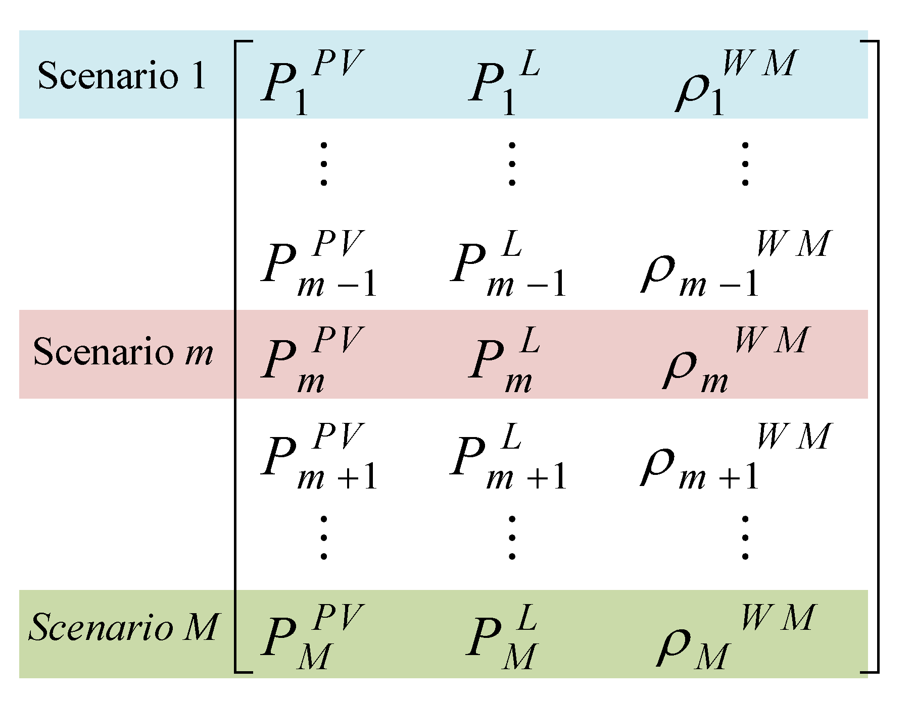
• Proposing a scenario matrix based on the HMM method to achieve the stochastic moments and correlations among the historical scenarios,
• Transforming the non-linear bi-level optimization problem into the single-level MISOCP optimization problem through linearization techniques and KKT optimality conditions.

The remainder of the paper is organized as follows: In Section 2, the scenario matrix is modeled. The bi-level optimization model of the problem is formulated in Section 3. Case study and simulation results are discussed in Section 4. Finally, the conclusions are drawn in Section 5.

2. Uncertainties Modelling

Due to the uncertainty nature of input data in the proposed distribution management system (DMS), stochastic operation scheduling is developed. First, the uncertainty matrix based on the HMM method is modeled. Then, appropriate transformations are used to find the stochastic moments and correlations among the historical scenarios.

Modeling of Scenario Matrix

In order to cover the uncertainty of input data such as electrical load demand, solar irradiance, and wholesale market prices, a scenario-based stochastic programming approach is implemented. In this paper, the HMM method [23] is used to model scenario matrix, including reduced number of scenarios, that can approximate the stochastic nature of the historical scenarios. Although a larger number of scenarios leads to a more accurate approximation of the original model, this could ascend the computational burden rapidly. A sample of scenario matrix comprising of M scenarios of solar irradiance, electrical load demand, and market prices is presented in Figure 1.

The HMM method employs the cubic transformation and the matrix transformation to achieve the stochastic moments and correlations, respectively. In this regard, as mentioned in [21], the first four stochastic moments i.e., expectation, standard deviation, skewness and kurtosis are selected to retain the stochastic features of scenarios. The HMM process can be discussed as follows:

Step 1: First, calculate the correlation matrix ($R$) and the target moments ($M_{i,k}^T$) of the hourly PV generations, electrical load demand, and market prices. Then, compute the related normalized values ($M_{i,k}^{NT}$) as follows:

$$\{\begin{array}{cc}{M}_{i,1}^{NT}=0,& M_{i,2}^{NT}=1\\ M_{i,3}^{NT}=\frac{M_{i,3}^T}{{\left(\sqrt{M_{i,2}^T}\right)}^3},& M_{i,4}^{NT}=\frac{M_{i,4}^T}{{\left(M_{i,2}^T\right)}^4}\end{array}$$

(1)

where, $i=1,2,3$ refer to the three considered uncertain parameters and $k=1,2,3,4$ refer to the first four stochastic moments.

Step 2: Randomly generate $N_m$ scenarios from $N_w$ uncertainty factors considering the normal distribution $N(0,1)$ to determine matrix $X_{N_m\times N_w}$[23].

Step 3: Employ the matrix transformation [23], as presented in (2), to satisfy the correlation matrix ($R$) by transforming $X_{N_m\times N_w}$ into the matrix $Y_{N_m\times N_w}$.

$$\{\begin{array}{l}Y=L\times X={\displaystyle \sum _{j=1}^i{L}_{ij}\times X_i}\\ R=L{L}^T\end{array}$$

(2)

where, L is a lower-triangle matrix of the correlation matrix that is determined by Cholesky decomposition [23].

Step 4: Utilize cubic transformation [23], as given in (3), to transform the standard normal random variable $Y_{N_m\times N_w}$ into a non-normal random variable $Z_{N_m\times N_w}$ to satisfy the normalized target moments of the historical scenarios.

$$Z_i={\alpha }_i+{\beta }_i{Y}_i+{\gamma }_i{Y}_i^2+{\lambda }_i{Y}_i^3$$

(3)

$$M_{i,k}(Z_i)=M_{i,k}^T$$

(4)

By considering (4), coefficients ${\alpha }_i,{\beta }_i,{\gamma }_i,{\lambda }_i$ are calculated in (3).

Step 5: calculate the correlation error (${\epsilon }_c$) and the moment errors (${\epsilon }_m$), as presented in (5) and (6), respectively. This algorithm converges to the solution when the amount of calculated errors are less than predefined thresholds given in (7).

$${\epsilon }_c={\displaystyle \sum _{i=1}^{N_m}\sqrt{\frac{2}{N_w(N_w-1)}{\displaystyle \sum _{i=1}^{N_f}{{\displaystyle \sum _{i=1}^{N_f}\left(R_{il}^G-R_{il}^{NT}\right)}}^2}}}$$

(5)

$${\epsilon }_m={\displaystyle \sum _{i=1}^{N_m}\left(\left|M_{i1}^G-M_{i1}^{NT}\right|+{\displaystyle \sum _{k=2}^4\left|M_{ik}^G-M_{ik}^{NT}\right|}/M_{ik}^{NT}\right)}$$

(6)

$${\overline{\epsilon }}_c=5\%,{\overline{\epsilon }}_m=5\%$$

(7)

Step 6: Calculate the scenario matrix ${\mathsf{\Omega }}^M$ containing scenarios of PV generation, electrical load demand, and market prices as follows [23]:

$${\Omega }^M=\sqrt{M_{i,2}^T}\times Z_i+M_{i,3}^{NT}$$

(8)

3. Problem Formulation

Firstly, the framework of the proposed bi-level optimization model considering correlations among uncertainties is summarized in Figure 2. Then, problem formulation of the bi-level optimization model and related solution methodology are described in the following subsections.

3.1. Upper-Level: Distribution System Operator (DSO) Decision Making

At this level the objective function is formulated to minimize the cost of DSO, which includes two cost terms as follows:

$$O{F}_{DSO}=Min\left[{\displaystyle \sum _{t=1}^{24}\left(C_t^{WM}+C_t^{MG-DSO}\right)}\right]$$

(9)

where, the first term denotes the cost of selling/purchasing power to/from the day-ahead wholesale market at time t represented by (10).

$$C_t^{WM}={\rho }_t{}^{WM}\times P_t{}^{WM-DSO}$$

(10)

The second term in (9) calculates the cost of exchanging power between DSO and MGs as follows:

$$C_t^{MG-DSO}={\rho }_t{}^{RM}{\displaystyle \sum _{p=1}^{N_{MG}}\left(P_t{}^{MGp-DSO}\right)}$$

(11)

Constraints

To achieve a stable operation of the DSO, the following constraints should be met.

• Bus voltage limits constraint:

  $$V_{\min }^{}\le V_{m,t}\le V_{\max }^{},v_{slack}=1$$

  (12)
• Line current limits constraint:

  $$I_{mn,t}\le I_{\max }^{}\forall (m,n)\in br$$

  (13)
• Exchanged power limit with the wholesale electricity market:
  In order to deal with the limited capacity of sub-transmission transformer, the exchanged power between the wholesale market and DSO should be guaranteed as follows:

  $$P_t^{WM-DSO}\le P_{\max }^{WM-DSO}$$

  (14)
• Exchanged power limit between DSO and MGs:
  Based on the aforementioned limitations in the contract for the exchanged power between DSO and MG operators, constraint (15) should be met.

  $$P_{\min }^{MG-DSO}\le P_t^{MGp-DSO}\le P_{\max }^{MG-DSO}$$

  (15)

3.2. Lower-Level: Multi-Microgrids (MMGs) Decision Making

The objective function of the lower-level optimization problem is formulated to maximize the profit of pth MG. For the sake of brevity in the formulation, the output power of PVs, MTs, and ESSs are aggregated as $P_{\omega ,t}^{DER}$. The considered objective function is as follows:

$${OF}_{MGp}=Max\left({Pr}_{p,t}^L{+Pr}_t^{MGp-DSO}{+Pr}_t^{MGp-MGq}{+Pr}_{p,t}^{DERs}\right)$$

(16)

Objective function (16) includes four profit terms represented in (17)–(20).

$${Pr}_{p,t}^L={\rho }_t^{RM}{\displaystyle \sum _{i\in {\psi }_p}^{}(P_{m,t}^L})$$

(17)

$${Pr}_t^{MGp-DSO}={\rho }_t^{RM}\times P_t^{MGp-DSO}$$

(18)

$${Pr}_{\mathrm{t}}^{MGp-MGq}={\rho }_t^{RM}{\displaystyle \sum _{q=1,q\ne p}^{N_{MG}}\left(P_t^{MGp-MGq}\right)}$$

(19)

$${\mathrm{Pr}}_{p,t}^{DERs}=-{\displaystyle \sum _{\omega \in MGp}^{}({\alpha }_{\omega }^{DER}{P}_{\omega ,t}^{DER}+{\beta }_{\omega }^{DER})}$$

(20)

Constraints

To achieve the stable operation of the MMGs, the following constraints should be considered in the scheduling model.

• Exchanged power limit between DSO and each MG:

$$P_{\min }^{MG-DSO}\le P_t^{MGp-DSO}\le P_{\max }^{MG-DSO}$$

(21)

• Exchanged power limit between MGp and MGq:

$$P_{\min }^{MGp-MGq}\le P_t^{MGp-MGq}\le P_{\max }^{MGp-MGq}$$

(22)

• Operation limit of MTs:

At any time, the output power of MTs should be within an allowable range.

$$P_{\min }^{MT}\le P_{\omega ,t}^{MT}\le P_{\max }^{MT}$$

(23)

• Operation limits of ESSs:

$$P_{\min }^{ESS}\le P_{\omega ,t}^{ch}\le P_{\max }^{ESS}$$

(24)

$$P_{\min }^{ESS}\le P_{\omega ,t}^{dch}\le P_{\max }^{ESS}$$

(25)

$$E_{\min }\le E_{\omega ,t}^{}\le E_{\max }$$

(26)

$$E_{\omega ,t}=E_{\omega ,t-1}+{\eta }_{\omega }^{ch}{P}_{\omega ,t}^{ch}-\frac{P_{\omega ,t}^{dch}}{{\eta }_{\omega }^{dch}},\forall t\ge 1$$

(27)

$$E_{\omega ,t}=E_{\omega }^{initial},\forall t=0$$

(28)

$$U_{\omega ,t}^{ch}+U_{\omega ,t}^{dch}\le 1$$

(29)

• Power balance of pth MG:

$${\displaystyle \sum _{\omega \in p}\left(P_{\omega ,t}^{DERs}\right)}-P_t^{MGp-DSO}-{\displaystyle \sum _{q=1,q\ne p}^{N_{MG}}\left(P_t^{MGp-MGq}\right)}={\displaystyle \sum _{\omega \in p}(}{P}_{\omega ,t}^L)$$

(30)

3.3. Solution Methodology

The amount of exchanged power between MMGs and DSO acts as the mutual variable between these two optimization levels. Thus, the proposed model in (1)–(30) is a bi-level optimization problem, in which suitable transformation methods should be employed to facilitate implementing the resulting model in commercial optimization packages. In this regard, as the lower-level problem is linear and convex, the KKT optimality conditions of the lower-level is utilized to transform the bi-level model into the single-level optimization problem. By implementing the complementary constraints, the optimization model becomes non-linear, which is easily linearized by big-M method as follows [16]:

$$C_{m,p,t,i}^z\le M{U}_{m,p,t,i}^z,\forall z=1,2,\dots ,12\forall m,p,t,i$$

(31)

$${\lambda }_{m,p,t,i}^z\le M(1-U_{m,p,t,i}^z),\forall z=1,2,\dots ,12\forall m,p,t,i$$

(32)

where, $M$ is a large positive number.

Finally, the resultant single-level MILP optimization problem can be solved by off-the-shelf software, such as GUROBI [24] and CPLEX [25].

4. Numerical Results and Discussion

In this section, the test system and working scenarios are introduced first. Then, simulation results of the proposed bi-level operation scheduling problem are discussed. Uncertainty modelling is implemented in MATLAB software and run on a computer with 2.6 GHz and 4 GB of RAM. Furthermore, the resultant single-level MILP problem is coded in the GAMS platform and solved by the CPLEX [25] solver.

4.1. Test System

The performance of the proposed bi-level model is investigated using an actual 84-bus 11.4 kV Taiwan Power Company (TPC) distribution system [1,26] with two substations and 11 feeders, as shown in Figure 3. As can be seen, this system includes three interconnected MGs. The DERs including PVs, MTs, and ESSs are utilized in the MMG system under study.

Ten PV panels of 500 kW with similar type and size are considered, where the predicted values of PV output powers can be found in [27]. Seven identical 2 MW REDOX batteries [28], as ESSs, are installed at buses 3, 18, 40, 50, 57, 67, and 79. Moreover, eight similar Capstone MTs [29] with the maximum output power of 5 MW and electrical efficiency of 29% are considered. All the technical parameters and the necessary characteristics related to DERs are presented in

Table 1. Required technical parameters [1].

Parameter	Value	Parameter	Value
$P_{\max }^{MGp-MGq}(MW)$	15	${\alpha }_{\omega }^{MT}(\$/MWh)$	65
$P_{\max }^{WM-DSO}(MW)$	36	${\beta }_{\omega }^{MT}(\$)$	13
$P_{\max }^{MGp-DSO}(MW)$	20	${\alpha }_{\omega }^{PV}(\$/MWh)$	1.3
$V_{min},V_{max}(p.u.)$	0.95, 1.05	${\beta }_{\omega }^{PV}(\$)$	5
Ii,j,max(kA)	1.8	${\alpha }_{\omega }^{ESS}(\$/MWh)$	2
$E_{\min },E_{\max }(MWh)$	0.5, 2	${\beta }_{\omega }^{ESS}(\$)$	2.5
${\eta }_i^{ch},{\eta }_i^{dch}(p.u.)$	0.92, 0.92	$P_{\min }^{ESS},P_{\max }^{ESS}(MW)$	1

[1]. The hourly total load demand and load profile of each MG during the scheduling day are shown in Figure 4 [1]. Moreover, the wholesale market and retail market prices for the whole 24-h scheduling horizon can be extracted from [1,16].

4.2. Simulation Results

In order to investigate the effect of wholesale market prices on the simulation results, three different case studies are defined. The proposed prices in [1] are defined as case study 1, while 10% decrement and increment in these amounts are considered as case study 2 and case study 3, respectively.

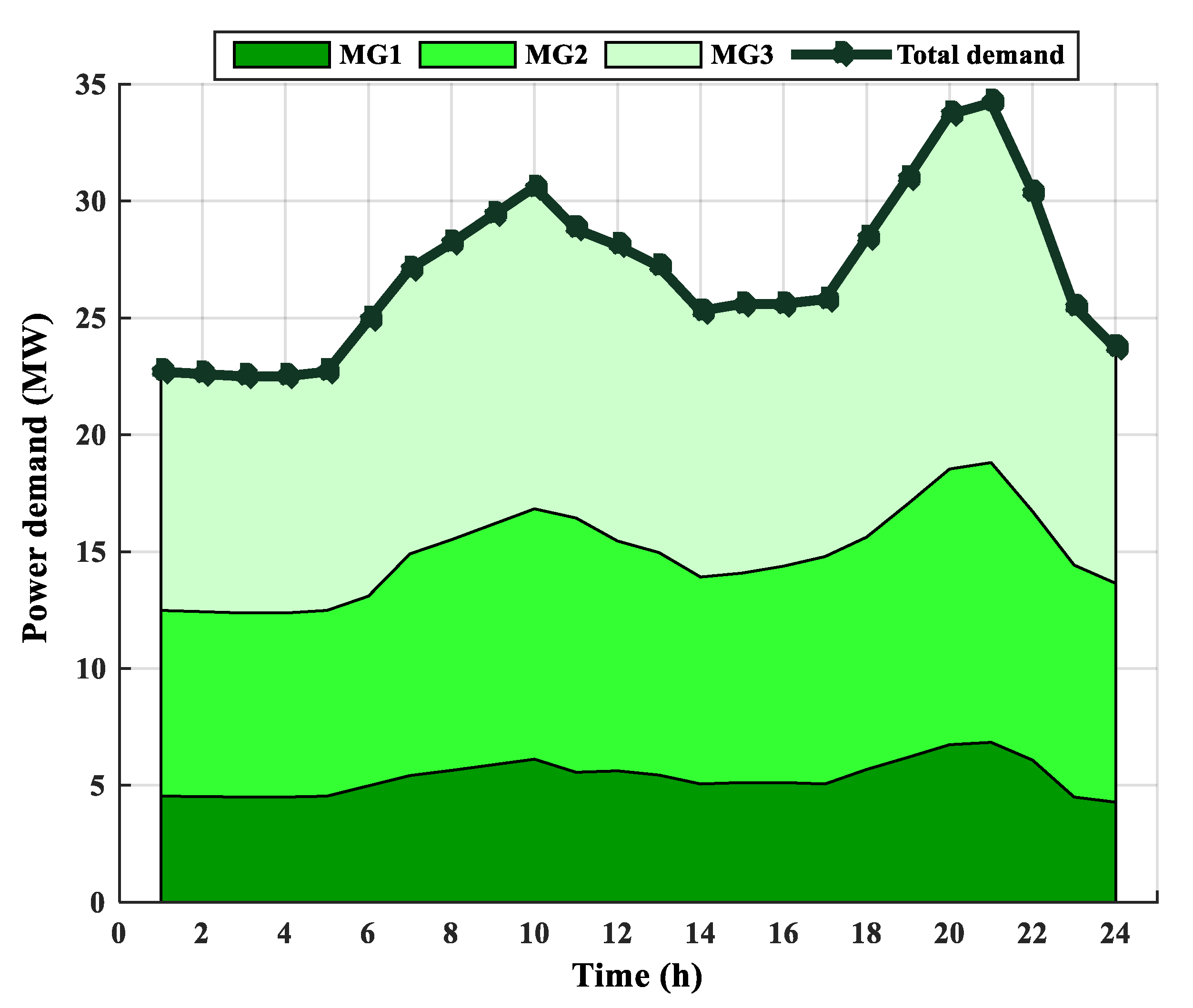
4.2.1. Operation Scheduling

Optimal operation scheduling of PVs, MTs, and ESSs for scenario 1 in MG1, MG2, and MG3 are proposed in Figure 5. As can be seen, ESSs in MGs store power during off-peak periods and discharge the stored power at peak hours (i.e., 10:00–12:00 and 20:00–22:00).

Due to the lower generation cost of MTs than the wholesale market price during peak load periods, MTs work at their maximum allowable power generation level. Furthermore, based on the power generation capacities and load demand of each MG, MG1 has excess power generation, where MG2 and MG3 have shortage power. In this regard, Figure 6 shows the amounts of exchanged power among MGs through retail electricity market to balance the shortage and excess of power generations. It is observed that MG1 sells power to MG2 and MG3, while MG3 purchase power from MG2 to meet the supply–demand balance.

4.2.2. Considering Uncertainties

In order to investigate the effect of uncertainties on the performance of the proposed approach in depth, three scenarios for the number of installed PV systems are defined. The number of PVs for base case, i.e., 10 PVs, are considered as Scenario 2 (SC2), while 2 and 50 installed PVs are considered as Scenario 1 (SC1) and Scenario 3 (SC3), respectively.

First, the 3-year (2015–2018) historical hourly data related to PV generation, electrical load demand, and wholesale market prices is extracted from [30]. Then, the HMM method is utilized to generate sufficient number of scenarios over the range of 10 to 100. By comparing the historical data with generated scenarios in Figure 7, the effectiveness of the HMM method is demonstrated for SC1, SC2, and SC3. It can be seen that as the amount of scenarios increase from 10 to 100, the amount of errors related to the first four stochastic moments (i.e., expectation (M1), standard deviation (M2), skewness (M3) and kurtosis (M4)) between the historical data and generated scenarios are reduced significantly. Thus, these results confirm that the generated scenario matrix represents the stochastic features of historical scenarios accurately. Although the number of installed PVs is increased in SC3, the moment of errors are controlled within an acceptable range (less than 6%) shown in Figure 7c.

Figure 8 shows the performance of the proposed approach regarding the number of scenarios. It can be seen that by increasing the number of scenarios, the total cost is decreased and the total execution time is increased. Moreover, when the number of scenarios reaches to a specific amount; thereafter, the amount of cost is decreased slightly and the execution time is increased significantly. Thus, 50 scenarios are selected as a trade-off between the execution time increment and cost reduction.

Table 2. Effect of correlations on economic analysis.

	Parameter	Case Study 1	Case Study 2	Case Study 3
Without Correlation (SC2)	Cost of DSO	71,418	73,926	69,104
	Profit of MG1	6314	6210	6411
	Profit of MG2	4788	4696	4859
	Profit of MG3	4006	3931	4082
With Correlation (SC2)	Cost of DSO	71,952	74,519	69,828
	Profit of MG1	6293	6195	6396
	Profit of MG2	4761	4676	4834
	Profit of MG3	3978	3903	4054
Without Correlation (SC3)	Cost of DSO	71,364	73,868	69,052
	Profit of MG1	6392	6297	6499
	Profit of MG2	4859	4753	4914
	Profit of MG3	4097	4026	4159
With Correlation (SC3)	Cost of DSO	71,973	74,482	69,578
	Profit of MG1	6357	6249	6451
	Profit of MG2	4812	4715	4867
	Profit of MG3	4043	3974	4102

investigates the effect of correlations on the amount of total costs for the three defined case studies. Although the amounts related to the cost of DSO and profits of MGs are changed slightly, less than 1%, the correlations among uncertainties should be considered. It can be seen that by considering the correlations among variables, the amounts of MG profits are decreased, where the amounts of DSO costs are increased in the three case studies. This is because by considering correlations, in order to deal with the worst scenario, the operation costs are increased. Moreover, the profits of MGs are increased in SC3 comparing to SC2 due to the more output power of PVs in SC3. It can be concluded from Table 2 that the profits of MGs are decreased in case study 2 compared to case study 1. Because in case study 2 the wholesale market prices are decreased, thus more purchased power from wholesale market and less DER generations lead to less profits of MGs. On the other hand, the profits related to MGs are increased in case study 3 compared to case study 1 due to the wholesale market price increment. For the same reason, the cost of DSO is increased in case study 2 and decreased in case study 3 compared to case study 1.

4.2.3. Large-Scale Test Systems

In order to evaluate the efficiency and scalability of the proposed approach, larger-scale systems with 119 buses [31] and 1300 buses [32] are employed. The IEEE-119 bus system has 5 MGs with 22.809 MW and 17.041 MVAr loads, where the IEEE-1300 bus system includes 14 MGs with 132.07 MW and 115.26 MVAr loads. As can be seen in

Table 3. Calculation time for large-scale test systems.

	84-Bus TPC	IEEE 119-Bus	IEEE 1300-Bus
Calculation time (s)	21.7	26.2	89.4
Average cost (k$)	71.42	105.29	1202.67

, the proposed approach finds the optimal solution point within an acceptable time, which indicates the scalability of the algorithm. Moreover, it can be concluded that the average operation cost is increased as the test system becomes larger.

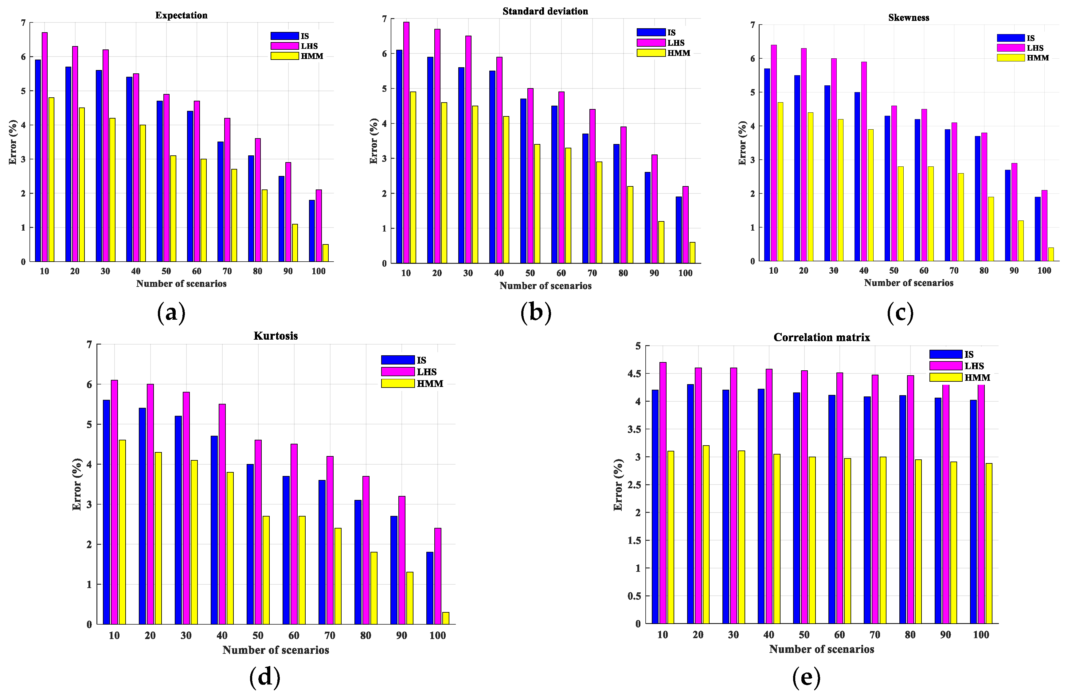
4.2.4. Performance Evaluation of the Proposed Heuristic Moment Matching (HMM) Method

In order to investigate the performance of the proposed HMM method, the errors of the first four moments and correlation matrix have been calculated and compared with the relevant results extracted from the Latin hypercube sampling (LHS) method [33] and the importance sampling (IS) method [34] over the range of 10 to 100 generated scenarios. The results are presented in Figure 9. As can be seen, the proposed HMM method performs much better than the other considered methods in terms of expectation, standard deviation, skewness, kurtosis, and correlation matrix errors. Moreover, as the number of generated scenarios increases, the errors of the first moments decrease. In contrast, it can be seen that the number of generated scenarios does not strictly affect the error of the correlation matrix, because the random data in the transforming method adjust the correlations among the scenarios.

5. Conclusions

This paper proposed the optimal operation scheduling problem of DSO and MMGs in the presence of uncertainties. In the addressed bi-level model, the upper-level problem minimized the total costs from the DSO’s perspective including the costs related to the exchanged power with the wholesale market and exchanged power between the DSO and MGs. For the lower-level problem, the profit of each MG including the profits related to the DERs, exchanged power between MGs and DSO, exchanged power among neighboring MGs, and the sold power to the loads was maximized. To tackle the uncertainty issue of input data such as electrical load demand, solar irradiance, and wholesale market prices, a scenario-based stochastic programming based on the HMM method was developed to build a scenario matrix with a reduced number of scenarios. The proposed approach effectively modeled the stochastic moments and correlation among the representative historical data. By applying KKT optimality conditions, the non-linear bi-level optimization problem was transformed into an MILP problem. To investigate the satisfactory performance of the proposed model, the 84-bus TPC distribution system was considered as a real case study. The simulation results revealed that the generated scenario matrix represents the stochastic features of historical scenarios accurately as the number of scenarios increases, the number of errors related to the first four stochastic moments between the historical data and generated scenarios is reduced significantly. It was shown that the correlations could affect the economy of the DSO and MGs by 1%. Besides, in case studies with the higher electricity market prices, MGs prefer to dispatch their owned DERs at the maximum allowable range, and then supply the probable shortage of power by purchasing the power from DSO and neighboring MGs. Moreover, the scalability of the proposed algorithm was evaluated by larger-scale systems with 119 buses and 1300 buses. Furthermore, the HMM method performed much better than LHS method and IS method over the range of 10 to 100 generated scenarios in terms of expectation, standard deviation, skewness, kurtosis, and correlation matrix errors.

References

1. Esmaeili, S.; Anvari-Moghaddam, A.; Jadid, S. Retail market equilibrium and interactions among reconfigurable networked microgrids. Sustain. Cities Soc. 2019, 49, 101628. [Google Scholar] [CrossRef]
2. Kou, P.; Liang, D.; Gao, L. Distributed EMPC of multiple microgrids for coordinated stochastic energy management. Appl. Energy 2017, 185, 939–952. [Google Scholar] [CrossRef]
3. Lv, T.; Ai, Q.; Zhao, Y. A bi-level multi-objective optimal operation of grid-connected microgrids. Electr. Power Syst. Res. 2016, 131, 60–70. [Google Scholar] [CrossRef]
4. Feijoo, F.; Das, T.K. Emissions control via carbon policies and microgrid generation: A bilevel model and Pareto analysis. Energy 2015, 90, 1545–1555. [Google Scholar] [CrossRef]
5. Vakili, R.; Afsharnia, S.; Golshannavaz, S. Interconnected microgrids: Optimal energy scheduling based on a game-theoretic approach. Int. Trans. Electr. Energy Syst. 2018, 28, e2603. [Google Scholar] [CrossRef]
6. Wang, Z.; Chen, B.; Wang, J.; Begovic, M.M.; Chen, C. Coordinated energy management of networked microgrids in distribution systems. IEEE Trans. Smart Grid 2014, 6, 45–53. [Google Scholar] [CrossRef]
7. Xie, M.; Ji, X.; Hu, X.; Cheng, P.; Du, Y.; Liu, M. Autonomous optimized economic dispatch of active distribution system with multi-microgrids. Energy 2018, 153, 479–489. [Google Scholar] [CrossRef]
8. Bahramara, S.; Parsa Moghaddam, M.; Haghifam, M.R. Modelling hierarchical decision making framework for operation of active distribution grids. IET Gener. Transm. Distrib. 2015, 9, 2555–2564. [Google Scholar] [CrossRef] [Green Version]
9. Bahramara, S.; Parsa Moghaddam, M.; Haghifam, M. A bi-level optimization model for operation of distribution networks with micro-grids. Int. J. Electr. Power Energy Syst. 2016, 82, 169–178. [Google Scholar] [CrossRef]
10. Tian, P.; Xiao, X.; Wang, K.; Ding, R. A hierarchical energy management system based on hierarchical optimization for microgrid community economic operation. IEEE Trans. Smart Grid 2015, 7, 2230–2241. [Google Scholar] [CrossRef]
11. Kim, H.-Y.; Kim, M.-K.; Kim, H.-J. Optimal operational scheduling of distribution network with microgrid via bi-level optimization model with energy band. Appl. Sci. 2019, 9, 4219. [Google Scholar] [CrossRef] [Green Version]
12. Esmaeili, S.; Khaloie, H.; Jadid, S.; Esmaeili, S. Optimal operation scheduling of a microgrid incorporating battery swapping stations. IEEE Trans. Power Syst. 2019, 34, 5063–5072. [Google Scholar]
13. Majidi, M.; Nojavan, S.; Zare, K. Optimization framework based on information gap decision theory for optimal operation of multi-energy systems. In Robust Optimal Planning and Operation of Electrical Energy Systems; Springer: New York, NY, USA, 2019; pp. 35–59. [Google Scholar]
14. Ji, L.; Zhang, B.; Huang, G.; Xie, Y.; Niu, D.-X. Explicit cost-risk tradeoff for optimal energy management in CCHP microgrid system under fuzzy-risk preferences. Energy Econ. 2018, 70, 525–535. [Google Scholar] [CrossRef]
15. Xu, S.; Sun, H.; Zhao, B.; Yi, J.; Hayat, T.; Alsaedi, A.; Dou, C.; Zhang, B. The integrated design of a novel secondary control and robust optimal energy management for photovoltaic-storage system considering generation uncertainty. Electronics 2020, 9, 69. [Google Scholar] [CrossRef] [Green Version]
16. Esmaeili, S.; Anvari-Moghaddam, A.; Jadid, S. Optimal operational scheduling of reconfigurable multi-microgrids considering energy storage systems. Energies 2019, 12, 1766. [Google Scholar] [CrossRef] [Green Version]
17. Kuznetsova, E.; Ruiz, C.; Li, Y.-F.; Zio, E. Analysis of robust optimization for decentralized microgrid energy management under uncertainty. Int. J. Electr. Power Energy Syst. 2015, 64, 815–832. [Google Scholar] [CrossRef]
18. Fioriti, D.; Poli, D. A novel stochastic method to dispatch microgrids using Monte Carlo scenarios. Electr. Power Syst. Res. 2019, 175, 105896. [Google Scholar] [CrossRef]
19. Ehsan, A.; Yang, Q. Scenario-based investment planning of isolated multi-energy microgrids considering electricity, heating and cooling demand. Appl. Energy 2019, 235, 1277–1288. [Google Scholar] [CrossRef]
20. Li, J.; Ye, L.; Zeng, Y.; Wei, H. A scenario-based robust transmission network expansion planning method for consideration of wind power uncertainties. CSEE J. Power Energy Syst. 2016, 2, 11–18. [Google Scholar] [CrossRef]
21. Ehsan, A.; Cheng, M.; Yang, Q. Scenario-based planning of active distribution systems under uncertainties of renewable generation and electricity demand. CSEE J. Power Energy Syst. 2019, 5, 56–62. [Google Scholar] [CrossRef]
22. Ehsan, A.; Yang, Q. Active distribution system reinforcement planning with EV charging stations—Part I: Uncertainty modeling and problem formulation. IEEE Trans. Sustain. Energy 2020, 11, 970–978. [Google Scholar] [CrossRef]
23. Høyland, K.; Kaut, M.; Wallace, S.W. A heuristic for moment-matching scenario generation. Comput. Optim. Appl. 2003, 24, 169–185. [Google Scholar] [CrossRef]
24. Gurobi Optimization. Available online: http://www.gurobi.com (accessed on 15 May 2020).
25. CPLEX Optimization Subroutine Library Guide and Reference; ILOG Inc.: Incline Village, NV, USA, 2008.
26. Esmaeili, S.; Jadid, S.; Anvari-Moghaddam, A.; Guerrero, J.M. Optimal operational scheduling of smart microgrids considering hourly reconfiguration. In Proceedings of the 2018 IEEE 4th Southern Power Electronics Conference (SPEC), Singapore, 12–13 December 2018. [Google Scholar]
27. Rabiee, A.; Sadeghi, M.; Aghaeic, J.; Heidari, A. Optimal operation of microgrids through simultaneous scheduling of electrical vehicles and responsive loads considering wind and PV units uncertainties. Renew. Sustain. Energy Rev. 2016, 57, 721–739. [Google Scholar] [CrossRef]
28. Carpinelli, G.; Celli, G.; Mocci, S.; Mottola, F.; Pilo, F.; Proto, D. Optimal integration of distributed energy storage devices in smart grids. IEEE Trans. Smart Grid 2013, 4, 985–995. [Google Scholar] [CrossRef]
29. Yinger, R. Behavior of Capstone and Honeywell Microturbine Generators during Load Changes; No. LBNL-49095; Lawrence Berkeley National Lab. (LBNL): Berkeley, CA, USA, 2001. [Google Scholar]
30. US. Energy Information Administration. Sources & Uses. Available online: https://www.eia.gov (accessed on 12 March 2020).
31. Fan, H.; Duan, C.; Zhang, C.-K.; Jiang, L.; Mao, C.; Wang, D. ADMM-based multiperiod optimal power flow considering plug-in electric vehicles charging. IEEE Trans. Power Syst. 2018, 33, 3886–3897. [Google Scholar] [CrossRef]
32. IEEE Test Feeders. Available online: https://ewh.ieee.org/soc/pes/dsacom/testfeeders/ (accessed on 15 March 2020).
33. Li, X.; Li, Y.; Liu, L.; Wang, W.; Li, Y.; Cao, Y. Latin hypercube sampling method for location selection of multi-infeed HVDC system terminal. Energies 2020, 13, 1646. [Google Scholar] [CrossRef] [Green Version]
34. Cai, J.; Xu, Q.; Cao, M.; Yang, B. A novel importance sampling method of power system reliability assessment considering multi-state units and correlation between wind speed and load. Int. J. Electr. Power Energy Syst. 2019, 109, 217–226. [Google Scholar] [CrossRef]
Figure 1. A sample of scenario matrix comprising of M scenarios.
Electronics 09 01441 g001
Figure 2. The framework of the proposed bi-level optimization model.
Electronics 09 01441 g002
Figure 3. The 84-bus Taiwan Power Company (TPC) distribution test system [1].
Electronics 09 01441 g003
Figure 4. Load profile of each microgrid (MG) and total demand [1].
Electronics 09 01441 g004
Figure 5. Optimal operation scheduling of distributed energy resources (DERs) for case study 1 in: (a) MG1; (b) MG2; (c) MG3.
Electronics 09 01441 g005
Figure 6. Amount of exchanged power among MGs.
Electronics 09 01441 g006
Figure 7. Amounts of moment errors between the historical data and generated scenarios for: (a) Scenario 1 (SC1); (b) SC2; (c) SC3.
Electronics 09 01441 g007
Figure 8. Performance analysis of the proposed approach regarding different number of scenarios.
Electronics 09 01441 g008
Figure 9. (a) Performance evaluation of the heuristic moment matching (HMM) method considering expectation, (b)standard deviation, (c) skewness, (d) kurtosis, and (e) correlation matrix errors.
Electronics 09 01441 g009