2.1. Establishment of a Robust 1D 1H-NMR-MS Protocol for Willow Metabolite Screening
We had established a number of years ago that 1D
1H-NMR profiling of extracts of freeze-dried Arabidopsis aerial tissue, made directly into deuterated methanol-water mixtures produced stable spectral fingerprints containing a range of primary and secondary metabolites that could define different genotypes [
21,
30,
31]. When this method was applied to wheat flour, a small modification, to incorporate a brief 2 min/90 °C heat shock, was added to the protocol in order to denature hydrolytic enzymes that remained active in the NMR samples causing spectral instability, particularly in carbohydrate signatures [
26]. This modified procedure has since been applied to over 100,000 samples of leaf, stem and seed tissues in our laboratory over recent years and has been described in detail [
32,
33]. The utility of this method is further enhanced as aliquots of the extract can be taken and diluted with non-deuterated solvent to provide parallel samples for mass fingerprinting by electrospray ionisation mass spectrometry (ESI-MS). These samples are totally compatible with the electrospray technique and can be infused directly into spectrometers and/or subjected to full LC-MS analysis. As the identical samples are used, correlative statistical analysis of 1D
1H-NMR
versus ESI-MS datasets has credibility and adds much confidence to biomarker discovery and structural determination (for example [
34]).
In initial experiments with willow, we utilised freeze-dried leaf and stem tissue, taken from three parts (top, middle, bottom) of the two biomass varieties, Tora and Resolution. Plant tissue was harvested, from field plots, in June in the middle of the rapid growth season, after coppicing in the previous February. It soon became apparent that 1D
1H-NMR fingerprints generated by our standard protocol (extraction at 50 °C in 80:20 D
2O:CD
3OD) [
32,
33] suffered from two problems: some peaks were poorly resolved and secondly many signals (compounds) common to all tissues were misaligned relative to added d
4-3-(trimethylsilyl)propionic acid (d
4-TSP) internal calibration standard (
Figure 1). The degree to which these two problems manifested themselves varied across the dataset. Misalignment of peaks was not a simple linear shift that could easily be dealt with by adding a data processing step. Binning or “bucketing” the 1D
1H-NMR spectra is a technique which is commonly utilised in metabolomics prior to downstream processing with statistical software. The technique reduces the resolution of the dataset to ensure that small changes in chemical shift between spectra do not yield false results from statistical processing of the data. The width (in ppm) of the “bucket” is chosen to try and ensure that a peak remains in its given bin or “bucket” despite small chemical shift variations between analyses. This can be achieved by using a user-defined fixed bucket width or via the use of intelligent bucketing [
35] which uses an algorithm to set the optimum bucket width for particular peaks such that they are not split between buckets. However, the extent of the variation in chemical shift for the distinctive anomeric hydrogen signals of sucrose and α-glucose (
Figure 1) was such that application of normal data processing strategies resulted in these abundant metabolites residing is different spectral buckets (bins).
Figure 1.
600 MHz 1D 1H-NMR willow leaf and stem spectra, from a polar solvent extraction using 80:20 D2O:CD3OD: illustrating chemical shift variation in anomeric sucrose (δ5.425–5.400) and glucose (δ5.225–5.195) signals together with shift variation and broadness in citrate and malate signals (δ2.75–2.30).
A fix based on processing with very wide bins (either via manual definition of the bucket size, or via intelligent bucketing) to encompass these shifts was not feasible as this resulted in signals from normally separated metabolites falling into the same bin, effectively reducing the high resolution spectra to a less useful, low resolution dataset with many uncertainties in metabolite annotation. The separate problem of poor resolution was also evident for a number of spectral regions particularly for the malate and citrate signals. In stem tissue samples, these signals could be easily observed but the degree of peak broadness varied for one sample to another depending on the harvest point of the willow stem. In leaves, the signals were so broad that they often seemingly disappeared into the baseline. The dual problem of variable line width and poor alignment meant that samples from different tissues or those taken from different parts of the plant could not easily be compared.
A similar problem has previously been observed in extracts of fruit tissue such as tomato and fruit juices [
36,
37] that contain varying levels of malic and citric acids. In fruit juices, the problem was easily rectified by adding buffer directly to the liquid sample. In tomato tissues the problem was overcome by modifying the protocol to add a dry-down step after the initial extraction and removal of aliquots for ESI-MS, followed by re-dissolution of the NMR sample in deuterated phosphate buffer. This stabilised the 1D
1H-NMR line shape and chemical shift of the organic acids as described by Kim
et al. [
38] and also realigned slight pH shifts in distinctive carbohydrate anomeric hydrogens. The willow spectra revealed that this plant also has high levels of citric and malic acids, but unfortunately, the relatively straight forward dry down/buffering solution to the problem was not completely successful (
Table 1). It is known that willow is unusual in that it accumulates high levels of calcium oxalate in leaf tissue [
39] and we reasoned that the 1D
1H-NMR alignment problems were due to complex interactions of calcium ions with a variety of organic acids in the matrix, including malate and citrate as well as the 1D
1H-NMR-invisible oxalate. To investigate this problem we carried out a detailed array of experiments as shown in
Table 1, involving buffering at different pHs and ionic strengths and the addition of variable amounts of EDTA to complex the calcium ions. Initial trials were carried out on a dried down polar extract (80:20 H
2O:CH
3OH) of plant tissue. Reconstitution in 300 mM sodium phosphate buffer at pH6 failed to align the 1D
1H-NMR peaks or to sharpen poorly resolved peaks such as those of citrate and malate. Increasing the ionic strength of the buffer to 600 mM still did not improve resolution. Trials were then carried out using EDTA to complex the Ca
2+ in the sample (
Table 1). Addition of 10 µL of a 3.2 mM solution of EDTA began to sharpen the pair of citrate doublets which appear between δ2.50 and 2.75. However the position of these peaks varied between samples. Adding increasing amounts (up to 100 µL) of the 3.2 mM solution of EDTA sharpened these peaks further but did not completely stabilise the chemical shift. Alternate strategies, to deal with Ca
2+, such as precipitation as CaF
2 following potassium fluoride addition [
40] or removal by chelation with solid cation exchange resins [
41] were also unsuccessful, failing to improve resolution or stability of peak position.
An alternate solution to re-dissolution of the dried extract in aqueous buffer was to reconstitute the sample in the same ratios of deuterated methanol-water solvents as used to extract the plant. This improved the efficiency of reconstitution. Buffering of this solution via the addition of a small concentrated (10 µL, 2.6 M) “slug” of pH 6.0 buffer to the final sample appeared to improve the alignment of most signals in the spectrum, excluding malate and citrate. Increase of the pH of the concentrated buffer additive to 7.4 or 8.0 resulted in good alignment of these signals. Sharpening of the citrate and malate signals, such that they were of a comparable resolution across different tissues and genotypes, also required the addition of EDTA and after further experimentation it was found that a 10 µL addition of a stronger solution (32 mM) worked most effectively. The addition of this EDTA solution however, required further adjustments to buffer concentration to re-align some signals. It was found that the addition of a further 10 µL portion of the 2.6 M buffer such that the final solution was supplemented with 10 µL 32 mM EDTA and 20 µL 2.6 M potassium phosphate (pH 7.4) was optimum.
Table 1.
Matrix of methods attempted to align and sharpen willow 1D 1H-NMR signals.
| Initial Extraction Solvent † | Dry Down Step | Reconstitution Solvent † (pH/Ionic Strength) | Additives ‡ | Spectral Quality |
|---|
| Additive | Final Concentration in NMR Tube | Peak Resolution (Citrate & Malate) | Peak Alignment (Citrate & Malate) | Peak Alignment (Other Peaks) |
|---|
| A | Yes | C (6.0/300mM) | None | N/A | Poor | Poor | No |
| A | Yes | C (6.0/600mM) | None | N/A | Poor | Good | No |
| A | Yes | C (6.0/600mM) | 10 µL 3.2 mM EDTA (D2O) | 45 μM | Good | Poor | Aligned within, but not across, tissues |
| A | Yes | C (6.0/600mM) | 30 µL 3.2 mM EDTA (D2O) | 131 μM | Good | Poor | Aligned within, but not across, tissues |
| A | Yes | C (6.0/600mM) | 50 µL 3.2 mM EDTA (D2O) | 213 μM | Good | Poor | Aligned within, but not across, tissues |
| A | Yes | C (6.0/300mM) | Cation exchange resin (Chelex 100, Na form) * | N/A | Poor | Poor | No |
| A | Yes | C (6.0/300mM) | 10 µL 2M KF (H2O) | 28 mM | Poor | Poor | Aligned within, but not across, tissues |
| A | Yes | C (7.0/300mM) | None | N/A | Poor | Poor | No |
| A | Yes | C (7.0/300mM) | 50 µL 3.2 mM EDTA (D2O) | 213 μM | Good | Poor | No |
| A | Yes | C (6.0/300mM) | 100 µL 3.2 mM EDTA (D2O) | 400 μM | Variable | Poor | No |
| B | No | N/A | 100 µL 3.2 mM EDTA (D2O) | 400 μM | Poor | Poor | Yes |
| B | No | N/A | 10 µL 32 mM EDTA (D2O) | 450 μM | Poor | Poor | No |
| A | Yes | B | 10 µL–2.6 M Potassium Phosphate Buffer (D2O), pH = 7.4 | 37 mM | Poor | Good | Yes |
| A | Yes | B | 10 µL–2.6 M Potassium Phosphate buffer (D2O), pH = 7.4; 10 µL–32 mM EDTA (D2O) | 36 mM (Pi) 444 μM (EDTA) | Good | Poor | Yes |
| A | Yes | B | 10 µL–2.6 M Potassium Phosphate buffer (D2O), pH = 8.0; 10 µL–32 mM EDTA (D2O) | 36 mM (Pi) 444 μM (EDTA) | Good | Good | Yes |
| A | Yes | B | 20 µL–2.6 M Potassium Phosphate buffer (D2O), pH = 8.0; 10 µL–32 mM EDTA (D2O) | 71 mM (Pi) 438 μM (EDTA) | Good | Poor | Yes |
| A | Yes | B | 20 µL–2.6 M Potassium Phosphate buffer (D2O), pH = 8.0; 20 µL–32 mM EDTA (D2O) | 70 mM (Pi) 865 μM (EDTA) | Good | Poor | Yes |
| A | Yes | B | 20 µL–2.6 M Potassium Phosphate buffer (D2O), pH = 7.4; 10 µL–32mM EDTA (D2O) | 71 mM (Pi) 438 μM (EDTA) | Good | Excellent (within a 0.01 ppm bin width) | Yes |
| B | No | N/A | 20 µL–2.6 M Potassium Phosphate buffer (D2O), pH = 7.4; 10 µL–32 mM EDTA (D2O) | 71 mM (Pi) 438 μM (EDTA) | Good | Excellent (within a 0.01 ppm bin width) | Yes |
In this way, a dataset was achieved within which all peaks from all tissue types were well resolved and aligned such that bucketing to 0.015 ppm reliably captured all the peaks in the same buckets between samples. By this approach we developed a protocol that produced stable, reproducible 1D
1H-NMR spectra whilst retaining the ability to remove aliquots of the original extract for ESI-MS. To prevent introduction of EDTA and buffer salts into ESI-MS samples, concentrated chelator and buffer solutions were added at the end of the process only to the NMR sample. Representative spectra from stem and leaf tissues are shown in
Figure 2. It can be seen that the organic acids are now well resolved and aligned, as are the anomeric hydrogens from common sugars. The signals from the Ca
2+ complex of EDTA are visible at 3.1 ppm (quartet) and 2.55 (singlet) [
42,
43] as abundant peaks, but do not interfere with those from endogenous metabolites. We can’t rule out the possibility that EDTA was also complexing with other paramagnetic and diamagnetic metal ions but characteristic 1D
1H-NMR peaks for e.g., Mg-EDTA (2.8 ppm) [
42] or Mn-EDTA (2.8 ppm) [
20] were not seen suggesting that Ca
2+ was the major cation responsible for chemical shift variation and peak broadening in willow tissues. Diamagnetic cations such as Ca
2+, are commonly associated with chemical shift variation due to their ability to bind to metabolites such as citrate [
40]. However, it is unusual for these diamagnetic cations to affect peak resolution which normally arises due to paramagnetic ion content. For example, studies in saliva showed that no peak broadening of the citrate peaks occurred due to the addition of additional Ca
2+ [
44]. In willow tissues it appears that the variable organic acid content in leaf and stem tissues coupled with a high calcium oxalate presence, especially in leaves is influencing not just peak position but also resolution of both malate and citrate peaks, a situation that varies with the age of the tissue and which cannot be rectified by buffering alone, instead requiring a careful balance of metal chelator addition and pH adjustment.
As the newly developed method involved a dry-down step, it also presented an opportunity to record the mass of extracted metabolites from each of the different tissue types. As shown in
Table 2 the total mass of metabolites extracted from standard aliquots of freeze-dried milled willow tissue varied with the location of sampling.
Table 2.
Level of extractable metabolite pool from S. viminalis leaf and stem tissue, expressed as a % of total dry biomass.
| Tissue and Position | Tora % Extractable | Resolution % Extractable |
|---|
| Leaf–Top | 26.9 ± 1.7 | 26.4 ± 2.6 |
| Leaf–Middle | 28.2 ± 1.7 | 31.6 ± 3.4 |
| Leaf–Bottom | 31.1 ± 1.2 | 30.0 ± 3.7 |
| Stem–Top | 32.00 ± 2.9 | 32.4 ± 2.3 |
| Stem–Middle | 18.3 ± 1.8 | 18.1 ± 1.8 |
| Stem–Bottom | 11.9 ± 1.7 | 13.8 ± 1.9 |
On the whole, approximately 30% of the dry mass of willow leaf was extractable, and this was consistent across both older and younger leaves. However, for stem tissue, not surprisingly, the percentage of extractable metabolites per unit dry weight of tissue, decreased from ca. 32% in stem tissue taken from the top of the plant to just 12% in stem material harvested from the bottom of the plant, reflecting the maturity and hardness of the wood from top to bottom. For qualitative analysis and relative quantitative analysis i.e., within sample or across samples of the same tissue type, the lower amount of extractives is not an issue. However, for the calculation of carbon pools and flow in different tissues around the plant then the extractable mass becomes a factor in any mass-balance analysis.
Figure 2.
Examples of leaf and stem 1D 1H-NMR data derived from extracts made using an:80:20 D2O:CD3OD extraction with final additions of 20 µL 2.6 M potassium phosphate buffer and 10 µL 32 mM ethylenediaminetetraacetic acid (EDTA) solutions in D2O. (a) Resolution-leaf-top; (b) Tora-leaf-middle; (c) Resolution-leaf-bottom; (d) Tora-stem-top; (e) Resolution-stem-middle; (f) Resolution-stem-bottom. 1: sucrose; 2: α-glucose; 3: β-glucose; 4: malate; 5: Ca-EDTA2−; 6: Ca-EDTA2−; 7: citrate; 8: succinate; 9: free EDTA.
A further issue that came to light during the development of the method concerns the flavan-3-ol catechin, which occurs widely in the plant kingdom, and is present at significant levels in willow samples. On standing in buffered deuterated aqueous solvents this compound undergoes slow hydrogen-deuterium exchange at the C-6 and C-8-positions.This results in loss of signal at δ6.09 (H-6) and δ 6.00 (H-8). Although less rapid than hydroxyl or carboxyl hydrogen exchange, the exchange of these aromatic hydrogen atoms, via keto-enol tautomerism, was a fairly fast process and as shown in
Figure 3, and was complete in 12 h at pH 7.4. The phenomena of H/D exchange have previously been reported in response to heating samples containing flavonoid metabolites [
45,
46] and also in related anthocyanin molecules in acidified methanolic or aqueous solutions [
47]. For the operation of the high throughput screen, varying degrees of exchange of the catechin H-6 and H-8 hydrogens, have potential to give false positive results in multivariate analyses of large sets of spectra. This can be avoided by either “resting” the samples for 12 h after addition of the buffer solution, before data collection, or, by removal of the affected chemical shift “bins” from the spreadsheet of chemical shift
versus intensity during data processing [
32]. This will prevent false discovery of catechin as a biomarker. Other non-exchangeable catechin aromatic hydrogens at δ6.93, 6.92 and 6.85, together with the aliphatic double doublet at δ2.86 (
Figure 3) can be diagnostic for this compound and thus should emerge from multivariate analysis if levels are changing across a sample set It should be noted that hydrogen-deuterium exchange in flavonoids only affects the buffered NMR sample. Samples for ESI-MS were removed before re-dissolution in NMR solvent and thus the flavonoids do not undergo any molecular weight shifts in this screen.
Figure 3.
600 MHz 1D 1H-NMR spectral regions from δ7.075–5.95 and δ3.05–2.70 to illustrate the position of stable and deuterium-exchangeable catechin signals of (a) freshly extracted willow leaf extract, (b) 12 h old willow leaf extract, (c) 12 h old catechin standard, (d) freshly extracted catechin standard.
2.2. Analysis of Tora and Resolution Using the New Method
Willow stems and leaves from the two biomass varieties Tora and Resolution were analysed using the protocol described above. The choice to analyse two biomass willow varieties which are genetically related was deliberately made in order to test the robustness of the newly developed extraction and data collection protocol. Unlike many other biomass willows, these two varieties have a very similar phenotype and metabolite changes due to genotype were expected to be subtle. The ability of a protocol to separate spectra arising from these genotypes relied on high quality analytical data with a low variation due to the method itself. Average relative standard deviations, describing variation in technical replication, for abundant metabolites identified in the leaf and stem 1D
1H-NMR spectra ranged from 2%–8% (
Table 3).
PCA of the resultant full 1D
1H-NMR dataset (
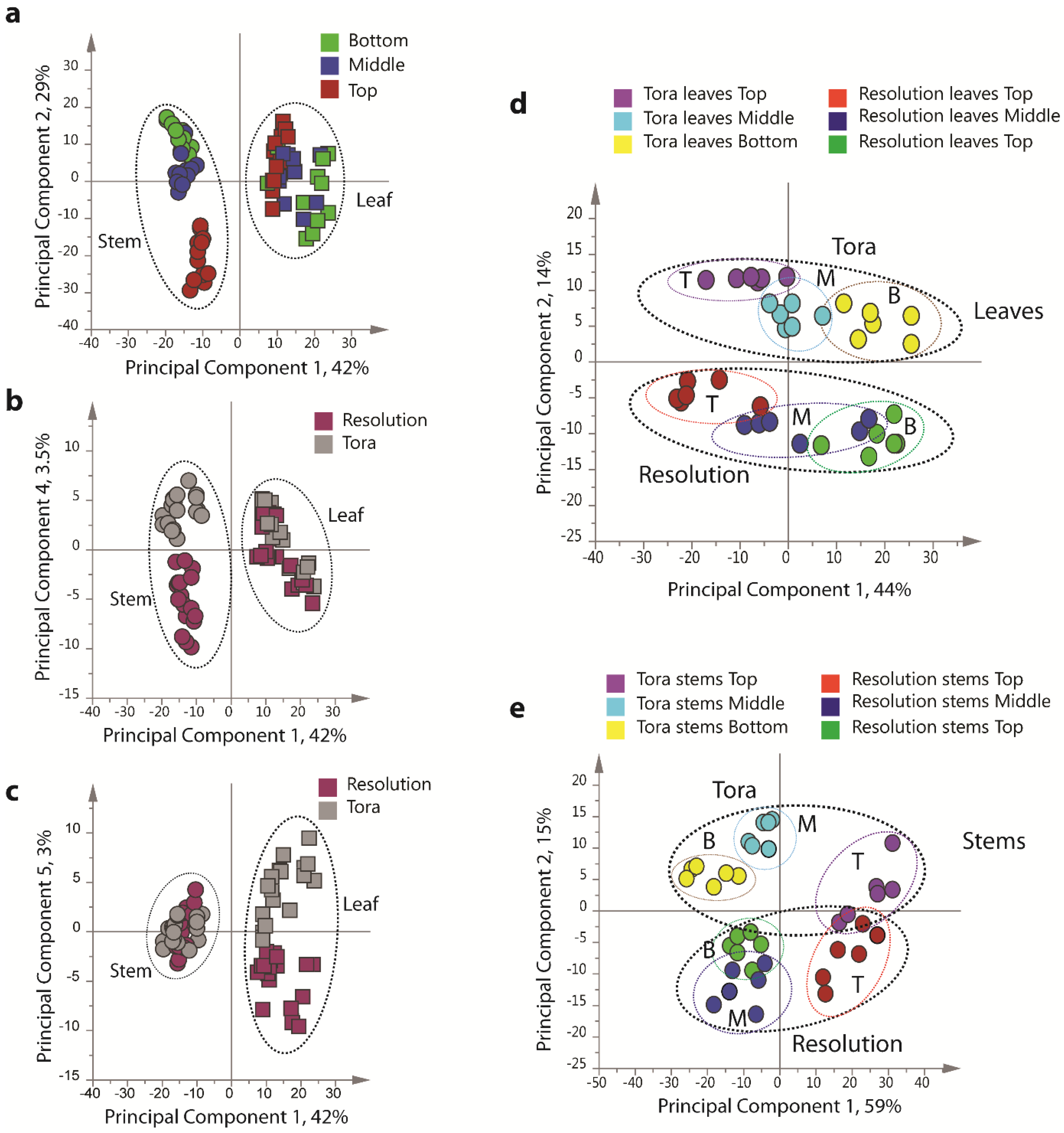
Figure 4), including all replicates, showed good clustering of the experimental data. Samples from technical and biological replicates for relevant samples clustered together and showed a lower variance compared to material from different sampling position or that from differing genotypes. Unsurprisingly the largest separation within the PCA model, in the direction of PC1 accounting for 42% of the total variance, was observed between leaf and stem samples (
Figure 4a) irrespective of genotype or sampling point. PC2, accounting for 29% of the variance, described the separation within the leaf or stem cluster, due to sampling point (top, middle or bottom of the plant). The impact of sampling point was greatest in stem samples where samples harvested from the top of the plant formed a distinct cluster. When coloured according to genotype, PC4, which accounted for 3.5% of the total variance, separated the two biomass lines in the stem samples (
Figure 4b).
Table 3.
Relative standard deviations (RSD) observed for characteristic metabolite regions in leaf and stem 1D 1H-NMR data. Data is based on three technical replicates per biological sample. Reported values represent the average % RSD observed across all leaf or stem samples. n.d. denotes a metabolite that was not quantified in a particular tissue.
| Metabolite | Leaves
% RSD | Stems
% RSD | Metabolite | Leaves
% RSD | Stems
% RSD |
|---|
| Sucrose | 2 | 3 | GABA | 8 | 4 |
| Glucose | 4 | 3 | Glutamine | 2 | 2 |
| Fructose | 2 | 2 | Alanine | 3 | 2 |
| Myo-inositol | 2 | n.d. | Threonine | 4 | 3 |
| Succinate | 6 | 7 | Valine | 5 | 5 |
| Citrate | 3 | 3 | Isoleucine | 6 | 4 |
| Malate | 2 | 2 | Leucine | 4 | 3 |
| Ascorbate | 4 | 7 | 2-Phenylethylamine | 5 | 4 |
| Quinate | 4 | 3 | Catechin | 2 | 7 |
| Lactate | n.d. | 3 | Dihydromyricetin | 3 | 8 |
| Aspartate | 4 | 8 | Gallocatechin | 3 | 8 |
| Asparagine | 7 | 4 | Chlorogenic Acid | 3 | n.d. |
In leaf samples, the two genotypes could be separated by PC5 accounting for 3% of the total model variance (
Figure 4c). When leaf and stem samples were analysed separately (
Figure 4d,e), clear clusters could be seen for sampling point in the direction of PC1 in both models. Separation due to genotype was evident in PC2. Interestingly, in stem tissue, the greater discrimination of samples was observed for tissues harvested from the bottom or middle of the plant. This discrimination was less evident in leaf samples where genotypes could be separated at all positional harvest points. Technical replication could also be assessed in the models resulting from separate tissue types (
Figure S1) and in general variance between the three technical replicates was lower than that observed between biological replicates.
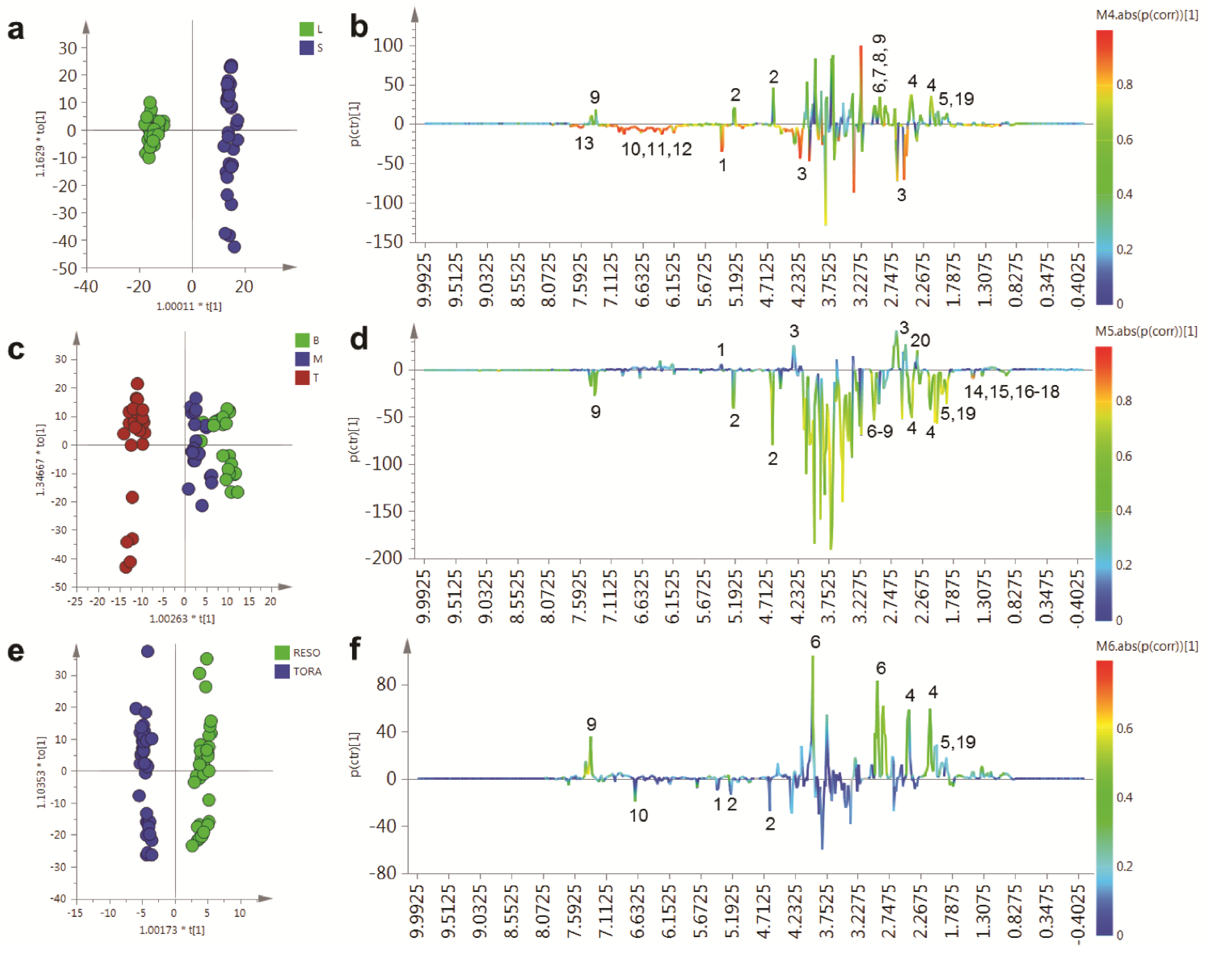
In order to determine the metabolites responsible for these distinct separations, a series of O-PLS models were constructed using a dummy matrix for separations due to tissue, sampling point or genotype (
Figure 5). Differences in the abundant metabolites between stems and leaves are shown in the OPLS S-plot in
Figure 5b. Stem tissues typically contain higher glucose than leaves. In addition a number of amino acids are elevated including glutamine, asparagine, aspartate and GABA. The aromatic metabolite 2-phenylethylamine, a metabolite formed from phenylalanine and which is dominant in juvenile willow tissues is more abundant in stem tissues. Finally, signals relating to quinic acid at δ 1.845–2.073 are present in both tissues but are elevated in stem tissues and are also discriminatory metabolites.
Figure 4.
PCA scores plots of binned 1D 1H-NMR data, indicating clustering of Tora and Resolution leaf and stem samples. (a) PC1 vs. PC2 of leaf and stem data, coloured by harvest position; (b) PC1 vs. PC4 of leaf and stem data, coloured by genotype; (c) PC1 vs. PC5 of leaf and stem data, coloured by genotype; (d) PC1 vs. PC2 of leaf data only, coloured by genotype and harvest position; (e) PC1 vs. PC2 of stem data only, coloured by genotype and harvest position. Harvest position: B:bottom; M:middle; T:top.
Contrastingly, leaf samples contain higher sucrose levels and elevated amounts of the organic acid malate. The abundant secondary metabolites, observed in leaves, included catechin and gallocatechin, while dihydromyricetin, the most abundant flavonoid in these
Salix genotypes, was higher in leaves compared to stem samples. Finally, chlorogenic acid, an ester formed from caffeic and quinic acids was detected only in leaf samples.
Figure 5c,d shows the OPLS model that describes metabolite changes observed due to location in the plant irrespective of tissue or genotype.
Figure 5.
OPLS analysis of binned 1D 1H-NMR data. (a) OPLS scores plot with Y variable as tissue type; (b) OPLS S-Line plot describing differences between stem (positive) and leaf (negative); (c) OPLS scores plot with Y variable as harvesting position; (d) OPLS S-Line plot describing differences between tissue harvested from the bottom of the plant (positive) and the top of the plant (negative); (e) OPLS scores plot with Y variable as genotype; (f) OPLS S-Line plot describing differences between Resolution (positive) and Tora (negative); Peak IDs: 1: sucrose; 2: glucose; 3: malate; 4: glutamine; 5: glutamate; 6: asparagine; 7: aspartate; 8: GABA; 9: 2-phenylethylamine; 10: dihydromyricetin; 11: catechin; 12: gallocatechin; 13: chlorogenic acid; 14: alanine; 15: threonine; 16: leucine; 17: isoleucine; 18: valine; 19: quinate; 20: citrate.
As can be seen from the S-line plot in
Figure 5d, a large number of signals are negative indicating that the abundance of the majority of extractable polar metabolites is typically higher in young leaves and stems taken from the top of the plant. Metabolites which oppose this, and that have higher concentrations in older tissue from the base of the plant, include sucrose, citrate and malate. Finally, the model constructed to describe generic differences between Tora and Resolution genotypes in shown in
Figure 5e,f. Resolution typically contains higher levels of glutamine, asparagine, 2-phenylethylamine, glutamate and quinic acid. In contrast, Tora samples are generally higher in the major carbohydrates sucrose and glucose. In addition, dihydromyricetin, the major flavonoid in these samples is elevated in the Tora genotype. The PCA and O-PLS models demonstrate that utilising the new extraction protocol, samples from different willow genotypes, where tissue has been obtained from different locations of the plant, can be separated on the basis of their tissue type, harvest point and genotype. O-PLS S-plots detail the major metabolites responsible for these separations. However, it was difficult to ascertain which quantitative metabolite profiles across the sampling position of the plant were able to discriminate the genotypes and which, if any, showed contrasting profiles in the leaf
versus stem tissue.
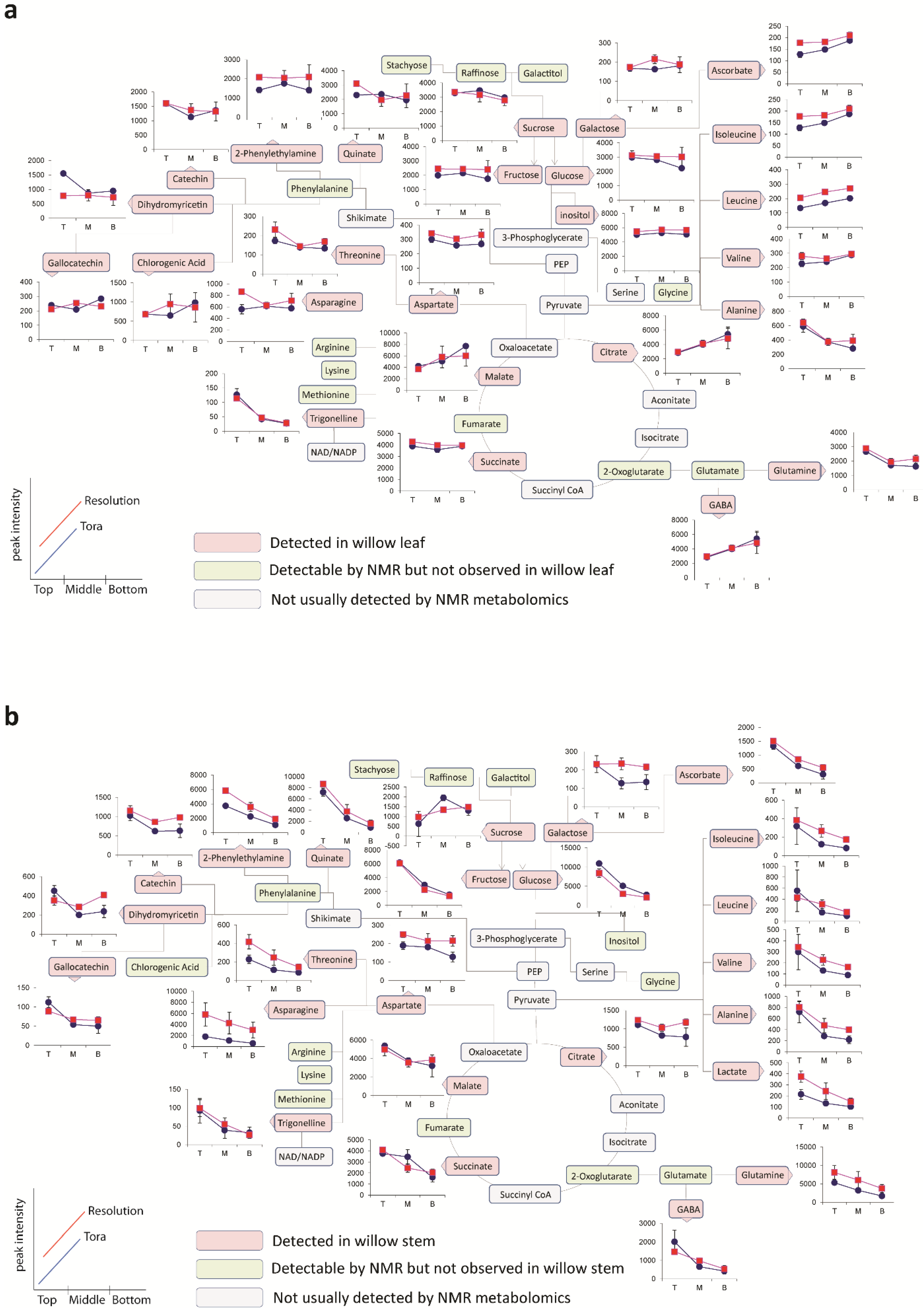
Figure 6 shows the metabolite trajectories across the height of the plant allowing differences in the profiles to be more easily discerned. In leaves, metabolite profiles (
Figure 6a) which discriminate Tora from Resolution include those of leucine, aspartate and 2-phenylethylamine. These metabolites show a similar trajectory but are typically more abundant in one genotype compared with the other. For other metabolites a difference between genotypes can be seen when tissue is harvested from a particular position of the plant. Clear differences in dihydromyricetin levels are observed when leaves are harvested from the top of the plant, but older leaves from the lower part of the plant are unable to discriminate the genotypes. Similar observations are seen for aspartate and glucose. In general, the major soluble carbohydrate concentrations decrease as leaves are sampled from the top to the bottom of the plants while organic acid concentrations (malic and citric) are higher in the lower older leaves. Similarly, the amino acids GABA, glutamine, valine, isoleucine and leucine show higher concentrations in these older leaves from the base of the plant. Contrastingly, alanine, glutamine and threonine levels reach their highest concentration in samples from the top of the plant.
Figure 6b shows the same type of metabolite profiles obtained from stem tissue. As suggested by the O-PLS plots, the extracted levels of many metabolites decrease in stem tissue obtained from the lower part of the plant. In many cases, although the profile follows the same trajectory the intensity of the profile is greater in material sampled from Resolution and examples here include asparagine, 2-phenylethylamine, threonine, isoleucine, lactate and glutamine. From this dataset the only metabolite that consistently increased when sampling the lower part of the stem was sucrose. This is in contrast to the profile observed in the leaves where sucrose was typically at its highest level when material was sampled from the top of the plant. Similarly the profiles of many amino acids and organic acids show contrasting profiles in the leaf and stem samples.
The data described in
Figure 6 was obtained via scaling the 1D
1H-NMR dataset to a known concentration of internal standard (d
4-TSP) which was present in the extraction solvent. Since 1D
1H-NMR is a quantitative technique, irrespective of metabolite chemistry, scaling to the internal standard gives information regarding the absolute concentration of metabolite extracted from 15 mg of dried plant sample. However, from the data in
Table 2 we know that the total amount of extractable metabolites is not consistent across all samples in the experiment. Whilst the mass of the soluble metabolome is fairly consistent in leaves and from stem samples obtained from the top of the plant, the amount of extractives obtained from older basal stem sections is considerably lower.
Figure 6.
Metabolite trajectories for (a) leaf and (b) stem samples. Data generated from 1D 1H-NMR data using binned regions for characteristic peaks for each metabolite. Plot intensities represent the intensity value of the binned region.
Thus, while
Figure 6 gives an overall picture of levels of each metabolite in each sample, it cannot describe relative changes within the soluble metabolite pool since some of these changes may be masked via a larger change in extractive yield. The new protocol described in this paper, incorporating a measurement of the extractives after dry down, allows the metabolomic 1D
1H-NMR data to be normalised to a constant sample weight. This reveals the spatial variation in the dataset allowing metabolite changes within the soluble metabolite pool to be discerned.
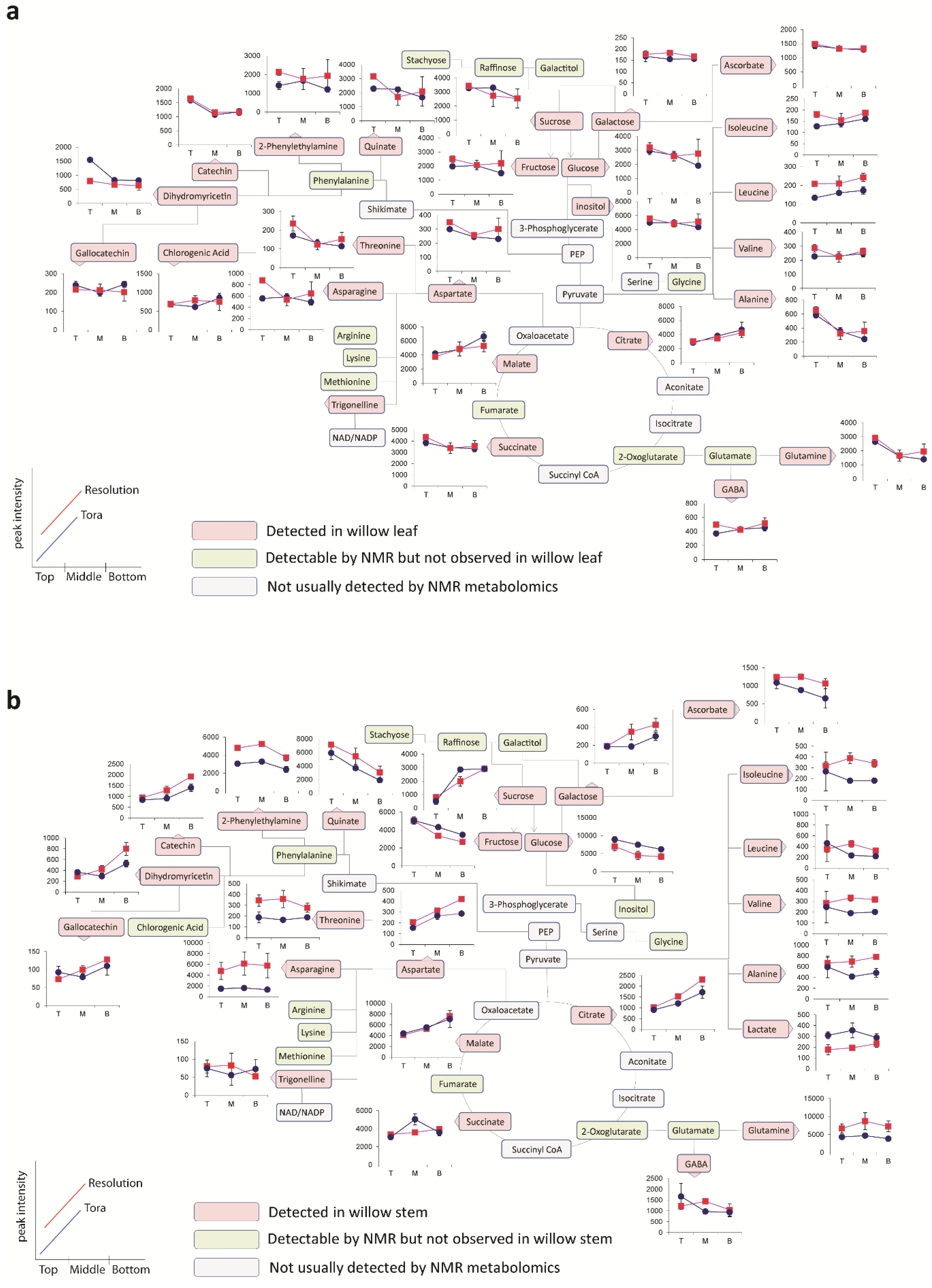
Figure 7 shows the effect of normalising the data back to a constant 3 mg weight of extractable material. The effect of the normalisation does not alter the direction of the leaf profiles (
Figure 7a). This is to be expected since leaves harvested from different parts of the plant typically yielded the same amount of extractable metabolites. However,
Figure 7b shows the effect of the normalisation of the stem data. Unlike the data displayed in
Figure 6b, which described the diminishing concentrations of the majority of soluble metabolites down the stem, this plot now shows a range of contrasting profiles and represents the real soluble metabolite changes happening within the part of the tissue, irrespective of a changing, and presumably increasing, non-extractable portion of the tissue sample. There is an approximately three-fold difference in the amount of extractives obtained between stems sampled from the top and bottom parts of the plant. Thus, the profile of any metabolite change which is within a three-fold difference may reverse its trajectory when normalised. Those which showed greater than three-fold changes will continue to show the same trajectory although the magnitude of that difference will be attenuated. For the abundant soluble carbohydrates (glucose, fructose and sucrose) the profiles show a similar trajectory to that previously described. However, there has been a large effect on the malate and citrate profiles which now show that both these metabolites actually increase in concentration
within the soluble metabolite pool as sampling proceeds from the top to the bottom of the plant. Similarly, we see that secondary products such as catechin, gallocatechin and dihydromyricetin increase in stem tissues obtained from the lower portion of the plant. In terms of differences between genotypes, the normalisation of the dataset to a constant weight of extractable metabolites shows that one of the largest differences in profile intensity is now observed for the asparagine content in stems which is very clearly higher in the material sampled from Resolution.
Examination of the direct infusion ESI-MS data from the top, middle and bottom sections of the two genotypes using PCA of the concatenated positive and negative ion spectra revealed that the data shape is in line with that seen for the 1D
1H-NMR profiles (
Figure S2). Leaf and stem samples could be easily separated in the direction of PC1 (45%) while PC2 (25%) separated the stem data based on sampling location (
Figure S2a). When coloured by genotype, PC4 (5%) separated the stem data based on genotype (
Figure S2b) and PC5 (1%) discerned differences due to genotype in the leaf samples (
Figure S2c).
When PCA models were constructed using stem or leaf data alone, the data further mirrored the clustering observed in PCA of the 1D
1H-NMR data (
Figure 4). In leaves (
Figure S2d), PC1 (81%) described the separation due to sampling point while PC2 (9%) separated the two genotypes. Samples taken from the top of the two different genotypes were easily differentiated. For the stem data only, (
Figure S2e), the ESI-MS data again mirrored the 1D
1H-NMR data (
Figure 4e) with harvest location described by PC1 (58%) and genotype described in the direction of PC2 (32%). Interestingly, it was more difficult to separate samples by genotype when material from the top of the plants was analysed by ESI-MS compared to samples taken from older, lower parts of the plant.
Figure 7.
Trajectories for (a) leaf and (b) stem samples representing changes within the extractable metabolite pool. Data generated from 1D 1H-NMR data using binned regions of characteristic peaks for each metabolite which were normalized back to a comparable 3 mg extractable pool weight. Plot intensities represent the intensity value of the normalized binned region.
This mirrored the observations from the PCA models constructed from stem 1D
1H-NMR data (
Figure 4e). Contrastingly, in the leaf only ESI-MS PCA model (
Figure S2d), the separation between middle and bottom harvest points was less discernible, when compared to the corresponding 1D
1H-NMR PCA model (
Figure 4d). However, on the whole the shape of the ESI-MS data matched that of the 1D
1H-NMR data, demonstrating that correlation of 1D
1H-NMR signal
versus ESI-MS signal is a valid strategy for metabolite annotation.
2.3. Construction and Application of a Bespoke Willow 1D 1H-NMR Spectral Library for Automated Quantitation of Metabolites
Provision of a list of metabolites in a sample with their concentrations is the output of choice for multidisciplinary projects where the data is to be mined against other trait or omics datasets or passed onwards for further statistical processing. The nature of 1D
1H NMR data and the complexity of typical plant extract spectra with many overlapping peaks from multiple metabolites make manual quantitation difficult and time consuming. Chenomx NMR suite is a set of tools for identifying and quantifying metabolites from 1D
1H-NMR spectra of mixtures [
48], allowing for quantitation of metabolites even when some signals are overlapped with those from another metabolite. Matching and quantitation can be carried out in automation based on comparison to a library of pH sensitive signatures of authentic metabolites run at differing instrument field strengths. However, as it was developed for clinical metabolomics, the Chenomx library does not contain many common plant metabolites, especially the species specific secondary metabolites. Furthermore, there is no capacity to compare spectra which have been collected in D
2O:CD
3OD mixtures. While this was a problem with some earlier versions of the software, Version 7.6 allows users to build user-defined signatures based on their own extraction protocol and 1D
1H-NMR data collection parameters. We have therefore constructed a library of signatures from all the abundant primary metabolites detected in Tora and Resolution willow leaves and stems and have supplemented this with signatures from key secondary metabolites such as flavonoids and phenolics and their glycosides, such as salicin and salicortin and triandrin, which are well documented in the
Salix literature. To date, this bespoke library contains 90 signatures, 52 of which overlap perfectly with those obtained when using the newly developed protocols described above. As an example, matching and quantitation (in μmoles/g dry weight and mg/g dry weight) of the Tora and Resolution leaf and stem data was evaluated and is detailed in
Tables S1 and S2. As can be seen by comparison with the data in
Figure 6, the use of the Chenomx profiling software has increased the number of metabolites that we were able to quantify. As a means of comparison to the relative data obtained from binning, quantified data in mg/g d.w. have been plotted across tissue types in
Figures S3–S6. The profiles of these concentrations agrees well with the majority of metabolites following the same trajectory as that obtained from plotting characteristic regions from the 1D
1H-NMR directly. Based on this quantified metabolite data, metabolites showing significant (
p < 0.05) differences between the Tora and Resolution genotypes could be identified in both stem and leaf tissues sampled at each part of the plant (
Table 4).
Table 4.
Metabolites showing a statistically significant difference between genotypes at varying parts of the willow plant in both leaf and stem tissue. Data is derived from a one-way ANOVA analysis of Chenomx-quantified metabolite concentrations derived from 1D 1H-NMR data.
| Differentiating Metabolite | p-value | Differentiating Metabolite | p-value | Differentiating Metabolite | p-value |
|---|
| Top of the plant | Middle of the plant | Bottom of the plant |
|---|
| Leaves | | | | | |
| Methionine | <0.00001 | Salicin | <0.00001 | Methionine | <0.00001 |
| Triandrin | <0.00001 | Uridine | 0.00052 | Lysine | 0.00004 |
| Asparagine | 0.00005 | Asparagine | 0.00061 | Tyrosine | 0.00006 |
| Raffinose | 0.00013 | 3-Hydroxymandelate | 0.00094 | Triandrin | 0.00009 |
| Uridine | 0.0003 | Leucine | 0.00276 | Lactic acid | 0.00027 |
| Citrate | 0.00044 | Glutamate | 0.0028 | Uridine | 0.0004 |
| Arginine | 0.00065 | Maltose | 0.00307 | Stachyose | 0.00053 |
| Dihydromyricetin | 0.00138 | 2-Phenylethylamine | 0.0033 | Glutamate | 0.00071 |
| Stachyose | 0.00141 | Gamma Aminobutyric acid | 0.00404 | Sucrose | 0.00102 |
| Succinate | 0.00174 | Glycine | 0.00422 | Leucine | 0.00398 |
| Tyrosine | 0.00243 | Succinate | 0.00727 | Asparagine | 0.00531 |
| Galactose | 0.00254 | Lactic acid | 0.01097 | Arginine | 0.00963 |
| Leucine | 0.00405 | Sucrose | 0.01543 | Succinate | 0.01145 |
| 3-Hydroxymandelate | 0.00506 | Dihydromyricetin | 0.02112 | Maltose | 0.01511 |
| 2-Phenylethylamine | 0.00722 | 2-Hydroxyisobutyrate | 0.02151 | 2-Phenylethylamine | 0.01618 |
| Lysine | 0.01531 | Chlorogenic Acid | 0.02225 | 3-Hydroxy-3-methylglutarate | 0.02667 |
| Maltose | 0.02151 | Tyrosine | 0.02266 | Gamma Aminobutyric acid | 0.02981 |
| Quinate | 0.02193 | Glutamine | 0.02382 | Acetate | 0.03418 |
| Salicin | 0.0232 | Stachyose | 0.03126 | Aspartate | 0.03775 |
| Glycine | 0.036 | Fumarate | 0.03775 | | |
| Chlorogenic acid | 0.03749 | | | | |
| Malate | 0.04741 | | | | |
| | | | | | |
| Stems | | | | | |
| Lactate | <0.00001 | Arginine | 0.000137 | Uridine | 0.00016 |
| Stachyose | 0.00002 | Raffinose | 0.000181 | Stachyose | 0.000274 |
| Succinate | 0.00038 | Sucrose | 0.001103 | Succinate | 0.001132 |
| Glycine | 0.00044 | Uridine | 0.001187 | Arginine | 0.00196 |
| Leucine | 0.00057 | Stachyose | 0.002002 | Glycine | 0.003298 |
| Tryptophan | 0.00123 | Lysine | 0.00206 | Methionine | 0.003722 |
| Raffinose | 0.00133 | Methionine | 0.002868 | Acetate | 0.004415 |
| Salicin | 0.00143 | Tyrosine | 0.005116 | Trigonelline | 0.01361 |
| Uridine | 0.00208 | Trigonelline | 0.005893 | Triandrin | 0.01569 |
| Dihydromyricetin | 0.00371 | Maltose | 0.006116 | Raffinose | 0.01611 |
| | | Glutamate | 0.007043 | Leucine | 0.01977 |
| | Dihydromyricetin | 0.008189 | Salicin | 0.01997 |
| | | 2-Phenylethylamine | 0.008416 | Lysine | 0.02147 |
| | | Glycine | 0.008923 | Valine | 0.02848 |
| | | Choline | 0.01115 | Lactic acid | 0.02986 |
| | | Gamma Aminobutyric acid | 0.0154 | Betaine | 0.0316 |
| | | Citric acid | 0.02168 | Maltose | 0.0436 |
| | | Leucine | 0.02354 | | |
| | | | | | |
There is surprisingly little published comparative quantitative data on
S. viminalis primary metabolites and thus it is difficult to compare the levels of individual metabolites or compound classes found in our study. Some other diverse Salix genotypes have been studied although often these studies have been sampled at different points in the developmental cycle, on other tissue types and are often subject to stresses or heavy metal treatments. Such examples include the assessment of amino acids in phloem and xylem of Salix species [
49,
50]. In the case of soluble sugars, glucose, sucrose and fructose have been described as the major soluble carbohydrates present in hydroponically grown, juvenile
S. viminalis leaves [
51] where levels reached 35 mg/g d.w. for glucose, 12.5 mg/g d.w. for fructose and 44 mg/g d.w. for sucrose. Our data from field grown tissue mirrors the profile in that glucose and sucrose levels were similar to each other in leaves harvested from the top of the plant and that fructose levels although still abundant were somewhat lower in concentration. The overall concentration of leaf soluble sugars appears lower in older field grown material compared to that reported for young plants. This is in agreement with data presented on
Populus deltoides ×
nigra where similar levels of carbohydrates were reported to our own study [
52].
In terms of organic acids, malate, citrate, ascorbate and quinate levels dominated the organic acids fraction of leaves in our study while major components in stems were ascorbate, malate, quinate and 2-oxoglutarate, the latter being highest from stem material harvested from the top of the plant. Malate and citrate levels (on a fresh weight basis) are reported in leaves of
S. alba at 1.6 and 0.6 mg/g F.W. respectively [
53]. Thus, our observations of 3–10 mg/g d.w. of citrate in leaves are broadly comparable. Similarly, results of 6–22 mg/g d.w. of malate in
S. viminalis are comparable with levels observed on a fresh matter basis in
S. alba leaves. Willow and poplar are well known for the diversity of phenolic glycosides present in stem tissues [
54], although it is also recognized that levels of such metabolites vary over the growth season [
55].
S. viminalis tissue is typically low in the salicinoids, during periods of active growth, compared to other varieties of willow such as
S. purpurea [
56]. Thus, as expected, we observed only small amounts of salicin (typically <1 mg/g d.w.) in this experiment. Additionally, the 1,4-substituted analogue triandrin was detected in all leaf and stem samples, consistent with previous findings [
56] that it is a common component in
S. viminalis. The aromatic regions of our spectra also contained a mixture of flavanols, with major components such as dihydromyricetin, catechin and gallocatechin. Levels of these compounds in our study ranged from 0.23–7 mg/g d.w. Such high levels of these compounds have previously been reported in stem tissues of e.g.,
S. caprea [
57].
Conversion of quantified data to units of mg/g d.w. allowed a total concentration of quantified metabolites to be elucidated (
Table S2). Of note here is the fact that, in leaf, the concentration of total quantified metabolites ranged from 75 mg/g d.w. to 93 mg/g d.w. and did not vary significantly by genotype or tissue position. This is in parallel with the data outlined in
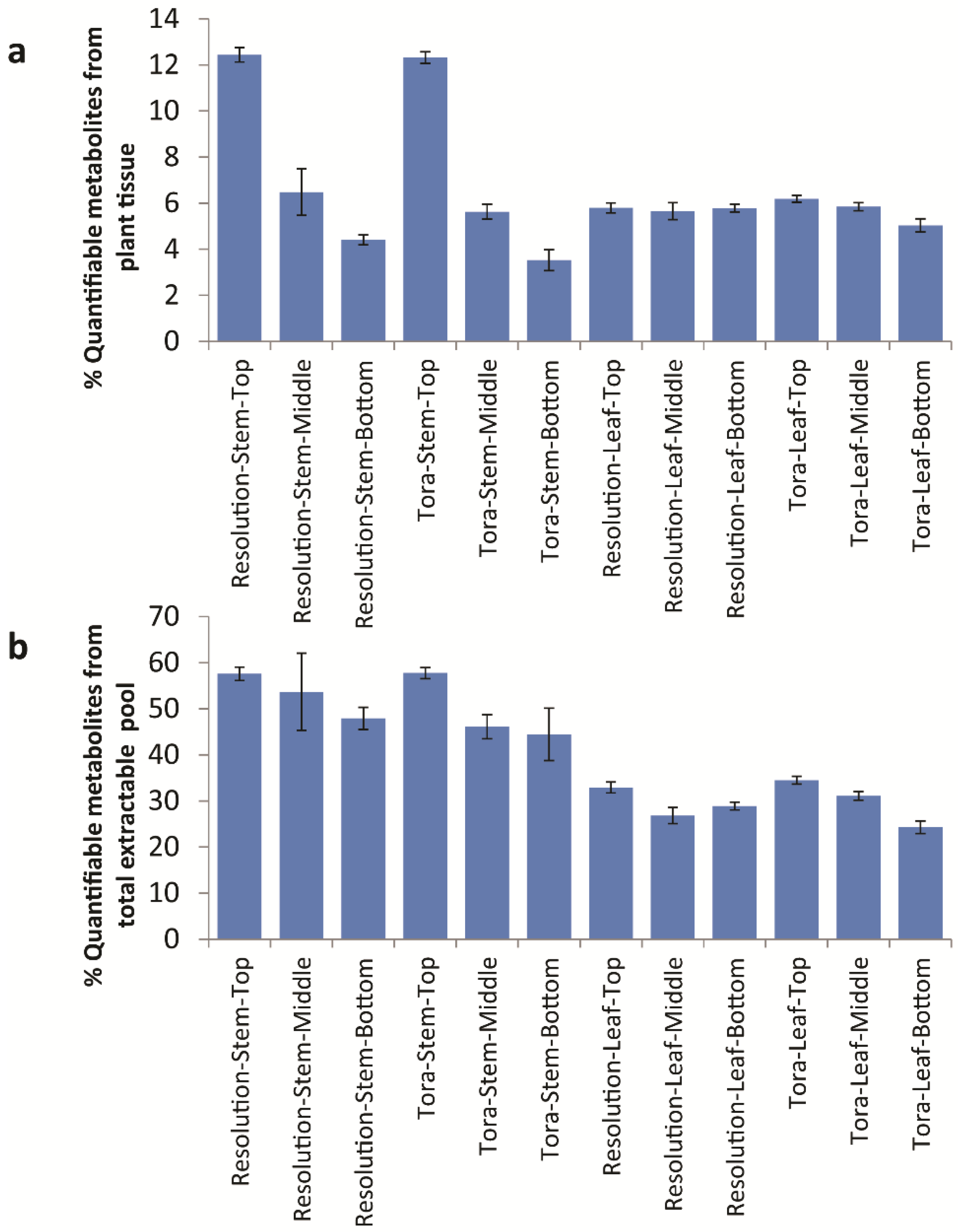
Table 2 relating to the variation in % extractable metabolites from leaf. However, 90 mg/g d.w. of quantified metabolites in leaf samples represents approximately 30% of the known extractable mass. Thus, in leaves, ~70% of polar extractives relate to unknowns that either have not yet been quantified or to substances that do not give signals in the 1D
1H-NMR spectrum (
Figure 8). Examples here would be inorganics such as phosphate, metal salts or oxalate (which is known to be high in willow leaves, [
29]) or multiple low abundance metabolites that are below the level of detection in NMR. From Chenomx assignments, it is the latter which is most likely. When compounds are examined by their chemical classes (
Figure 9), it is clear to see that the only class that changes in the absolute amount per gram of leaf tissue is the organic acids which are at their highest level in older leaves at the bottom of the plant.
Figure 8.
Calculated quantifiable metabolites (%) as a proportion of (a) total plant tissue and (b) total soluble metabolite pool. Data obtained from Chenomx quantification of metabolites as measured by 1D 1H-NMR.
Figure 9.
Calculated levels of compound classes via Chenomx quantification of metabolites as measured by 1D 1H-NMR. (a) Class levels expressed as mg/g dry weight; (b) expressed as a percentage of the total soluble metabolite pool.
When metabolite concentrations were normalised to the metabolite pool, we can also see that total levels of amino acids, carbohydrates and aromatics are highest in young leaves from the top of the plant. In contrast, mass that is 1D
1H-NMR invisible such as inorganic salts is lowest in young leaves. In stem tissues the absolute amount of metabolites that can be quantified per gram of plant tissue decreases (
Figure 8). However, within the pool the % of these quantifiable metabolites is relatively static. In terms of 1D
1H-NMR invisible metabolites, these are lowest in material from the top of the plant and increase in older stem tissue, although even here the mass of such metabolites is lower than seen in leaf material (
Figure 9). In terms of stem organic acids, these show a similar behaviour in both genotypes with highest levels at the top of the plant. In contrast to leaves, organic acid concentrations are lowest from stem material collected from the bottom of the plant. Levels of total soluble carbohydrates and amino acids discriminate genotypes with Tora containing higher stem carbohydrate and Resolution higher stem amino acids. Total aromatic metabolites are similar in both genotypes with highest levels of these compounds isolated from younger tissue. The development of the Chenomx metabolite library in concert with the methods described for sample handling and data collection therefore enable a detailed list of metabolites to be generated in high throughput for comparison of metabolite pools and compound classes between samples and will enable future large scale metabolomics experiments, such as mQTL studies, in willow.


