
Combining Empirical and Physics-Based Models for Solar Wind Prediction


Computer Science Department, Utah State University, 0500 Old Main Hill, Logan, UT 84322-0500, USA
*
Authors to whom correspondence should be addressed.
Universe 2024, 10(5), 191; https://doi.org/10.3390/universe10050191
Submission received: 25 February 2024
/
Revised: 3 April 2024
/
Accepted: 19 April 2024
/
Published: 24 April 2024
(This article belongs to the Special Issue Solar and Stellar Activity: Exploring the Cosmic Nexus)
Abstract
:Solar wind modeling is classified into two main types: empirical models and physics-based models, each designed to forecast solar wind properties in various regions of the heliosphere. Empirical models, which are cost-effective, have demonstrated significant accuracy in predicting solar wind at the L1 Lagrange point. On the other hand, physics-based models rely on magnetohydrodynamics (MHD) principles and demand more computational resources. In this research paper, we build upon our recent novel approach that merges empirical and physics-based models. Our recent proposal involves the creation of a new physics-informed neural network that leverages time series data from solar wind predictors to enhance solar wind prediction. This innovative method aims to combine the strengths of both modeling approaches to achieve more accurate and efficient solar wind predictions. In this work, we show the variability of the proposed physics-informed loss across multiple deep learning models. We also study the effect of training the models on different solar cycles on the model’s performance. This work represents the first effort to predict solar wind by integrating deep learning approaches with physics constraints and analyzing the results across three solar cycles. Our findings demonstrate the superiority of our physics-constrained model over other unconstrained deep learning predictive models.
1. Introduction
With the ever-growing interest in space exploration and the steady increase in the frequency of commercial flights, the importance of space weather prediction is becoming increasingly paramount. One of the recent executive orders issued by the United States highlights the importance of space weather research and calls upon scientists to prioritize the development of a comprehensive response plan for addressing severe space weather events [1]. While Earth’s magnetic field serves as a protective shield, safeguarding us against cosmic radiation and charged particles, certain particles can still penetrate our atmosphere and pose risks to communications, satellites, and the well-being of astronauts in space. For example, Solar Energetic Particles (SEP) can penetrate instruments on satellite instruments and potentially cause magnetic saturation, thereby resulting in electrical failures. Coronal Mass Ejections (CMEs) can induce currents in surface-based electronics which can overload terrestrial power grid operations. Moreover, X-rays from the Sun heat the Earth’s outer atmosphere, leading to its expansion, subsequently intensifying the drag force on satellites in low orbits. Consequently, space weather will also affect individuals dependent on technologies like satellite-based internet, the Global Positioning System (GPS), and weather forecasting services.
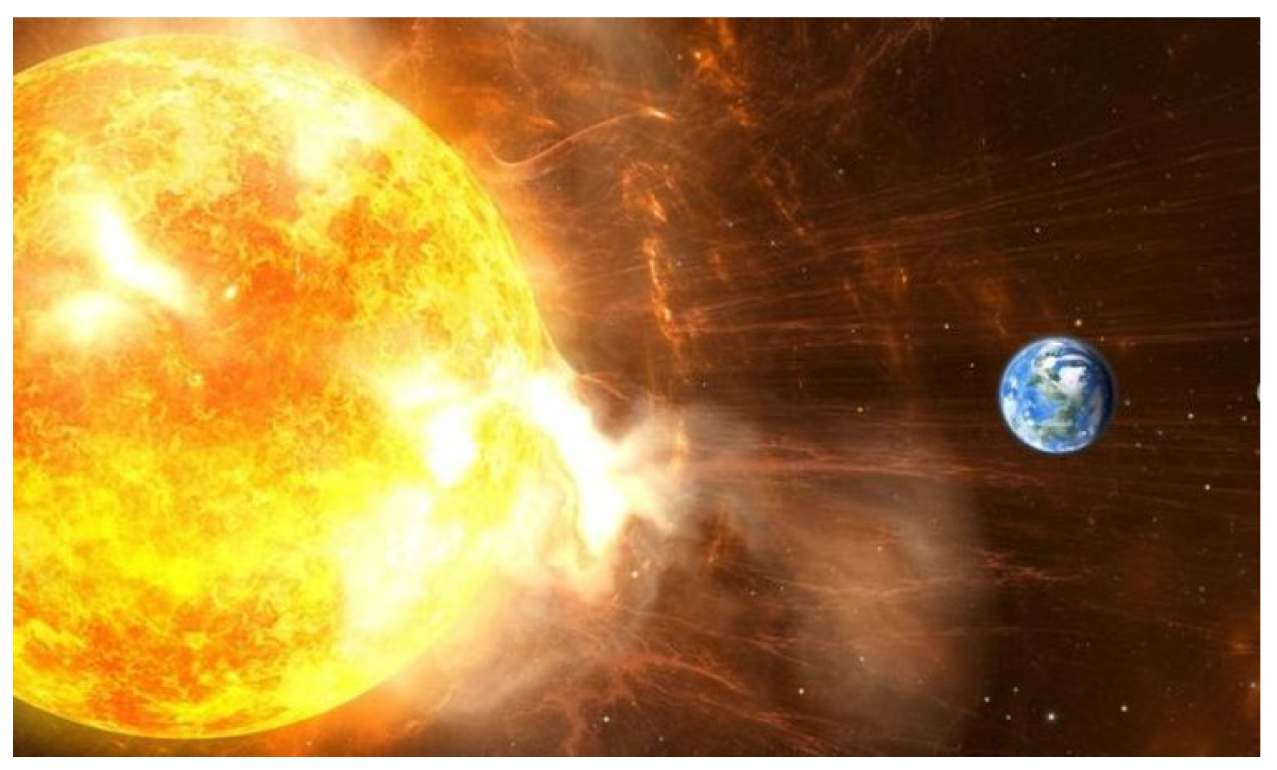
Another significant space weather phenomenon is solar wind (Figure 1) which consists of a charged matter stream originating from the sun. Accurate solar wind forecasts are crucial for safeguarding satellite integrity and astronauts’ health. Moreover, such forecasts can provide valuable insights into the underlying physical processes governing solar wind acceleration and composition. Under specific conditions, solar wind plasma behaves as an ideal plasma, where electrostatic forces dominate plasma motion more than ordinary gas kinetics [2]. While previous efforts mainly rely on solar condition measurements to predict solar wind characteristics, less attention has been given to data-driven prediction methods. The novelty of this research lies in its utilization of multivariate time series data, incorporating physics constraints suitable for ideal plasma to predict solar wind characteristics.
The rest of this paper is organized as follows: In Section 2, we discuss solar wind prediction efforts from the literature. In Section 3, we present the dataset used in this study and the data pre-processing pipeline. In Section 4, we defined the Ohm’s law constraint that we use to build our methodology. Section 5 discusses the details of the deep learning models used to predict solar wind, followed by Section 6 which lays the ground of our experimental setup. In Section 7, we discuss our findings. Finally, in Section 8, we conclude with a summary of our findings, highlight the contributions of our study, and we discuss potential future research directions on SEP events prediction.
2. Related Works
Since the discovery of solar wind over a century ago, a number of studies have been conducted to predict solar wind [4]. The predictive models can be categorized into three main categories: (1) empirical, (2) physics-based, and (3) data-driven models.
Empirical methods are based on statistical relationships derived from observational data. They use historical solar wind measurements to establish correlations between various solar and interplanetary parameters. Empirical models often consider factors such as solar wind speed, density, and magnetic field strength. The Wang-Sheeley-Arge (WSA) model is an example of a solar wind prediction model that falls under the category of empirical models [5]. To make predictions, the WSA model utilizes measurements of the Sun’s magnetic field at the photosphere, typically obtained from solar magnetograms. These measurements provide information about the magnetic field’s strength and polarity. The model then extrapolates this information to estimate the solar wind speed at 1 AU. Empirical Solar Wind Forecast (ESWF) is another algorithm which relies on an empirical correlation discovered between the size of solar coronal holes (CHs), observed in EUV, and the solar wind speed measured in situ at a distance of 1 AU from the Sun [6]. The main limitation of empirical methods is their reliance on observed data and statistical correlations rather than underlying physical principles or fundamental equations that increase the models’ interpretability.
Physics-based solar wind prediction models are based on fundamental physical principles that describe the behavior of the solar wind and its interaction with the Sun’s atmosphere (e.g., [7]). These models aim to simulate and forecast the properties and dynamics of the solar wind. Magnetohydrodynamic (MHD) models are highly adopted physics-based solar wind prediction models that simulate the solar wind by solving the MHD equations, which describe the behavior of magnetized plasmas. These models take into account the Sun’s magnetic field, its interaction with the solar corona, and the resulting propagation of the solar wind. MHD models can capture the large-scale structures and dynamics of the solar wind and provide insights into CMEs and other transient events. The ENLIL model is a three-dimensional MHD model, developed by a team of researchers at the NASA Goddard Space Flight Center, that simulates the propagation and evolution of CMEs and other solar wind phenomena in the heliosphere [5]. It provides forecasts of solar wind parameters such as speed, density, and magnetic field strength at different locations in space [8]. Wang-Sheely-Arge Enlil (WSA-Enlil) is a hybrid model that combines the Wang-Sheely-Arge empirical solar wind model with the Enlil three-dimensional MHD model to simulate the propagation and evolution of the solar wind as it expands outward from the Sun. A number of incremental works that build on the WSA-Enlil have been proposed. The increment is performed either by slightly improving the accuracy of the model, or by enhancing the efficiency of MHD equation computations for faster processing [9]. Shugai [10] proposed an improved WSA-Enlil by approximating the MHD computation through key assumptions. The enhanced WSA-Enlil model successfully transformed a three-dimensional problem into a one-dimensional problem, while maintaining a high level of accuracy [9]. Shugai [10] focused their modeling only on predicting the slow solar wind, as the fast solar wind can be more readily forecasted by examining the sizes of its sources, specifically coronal holes. Yang and Shen [11] introduced an innovative 3D magnetohydrodynamics (MHD) model that incorporates self-consistent boundary conditions derived from multiple observations. Their results demonstrate improved agreement with OMNI and Ulysses observations, surpassing previous MHD models relying solely on photospheric magnetic field data. Finally, Luo et al. [12] introduced a novel forecasting model that utilizes the presence of dark areas on the sun to generate accurate solar wind forecasts. Although physics-based models provide provide insights into the underlying mechanisms governing solar wind dynamics, they require accurate input data and computational resources to effectively simulate the complex interactions and dynamics of the solar wind system.
Data-driven models represent the third category of solar wind prediction, where patterns and relationships extracted from the data are utilized instead of depending on pre-determined rules or assumptions. Upendran et al. [13] was the first group to perform solar wind forecasting with interpretable ML methods, quantifying the effect of source regions. This study trains deep learning models on solar corona images to forecast solar wind speed. The models achieve a strong correlation of 0.55 with NASA’s OMNIWEB dataset and reveal patterns linking coronal features to wind behavior, potentially uncovering novel heliophysics relationships. Another example of data-driven methods is the work of Yang and Shen [14], who introduced neural network approaches that achieved superior forecasting results at 2.5 solar radii. Their approach utilized a three-layer fully connected network to establish the relationship between the polarized magnetic field, electron density, and solar wind velocity. Subsequently, the same group enhanced their method by incorporating self-consistent boundary conditions. Additionally, Raju and Das [15] developed an online model based on convolutional neural networks, trained on solar images, to gain a comprehensive understanding of solar activity for the prediction of solar wind velocities. Furthermore, Leitner et al. [16] made an intriguing discovery, demonstrating that the distribution of solar wind exhibits quasi-invariant characteristics. Sun et al. [17] leverage NASA’s OMNI data and SDO satellite image data to train a two-dimensional attention mechanism (TDAM) model for solar wind speed prediction. The primary challenge of data-driven methods lies in their potential to overfit the training data, resulting in reduced generalization performance [18]. Overfitting occurs when a model captures noise or irrelevant patterns in the training data, leading to poor performance on new, unseen data. To address this limitation, we build upon our previous work presented in [19], where we propose the utilization of a physics-informed neural network (PINN) [20,21] as a novel approach for solar wind prediction. Some recent studies have explored the use of PINNs for solar corona modeling and prediction. Zhao et al. [22] introduced the mutually embedded perception model (MEPM), a feed-forward neural network that reconstructs the structure of the solar corona based on observational data and by integrating the first-principle 3D magnetohydrodynamic governing equations of solar wind plasma. The authors first tested MEPM on an artificial analytic solution and showed that it is able to approach the exact situation in less than half of the modeling time. In addition, MEPM was able to provide good approximations of the 1D steady Parker flow and of the steady corona structure (from the CR 2068 modeling results). Jarolim et al. [23] proposed a physics-based neural network to extrapolate the coronal magnetic field. The model integrates the physical equations of nonlinear force-free magnetic fields as an approximation to the magnetized plasma under coronal equilibrium conditions to solve the boundary-value problem. The results of the model were validated through a simulation of active region NOAA 11158. In this paper, we delve into a comprehensive analysis of the role of solar cycles on the phenomenon, as well as an in-depth study of the Ohm’s law effect on deep learning baselines. Specifically, our contributions are summarized as follows:
- We present a more comprehensive and in-depth analysis of the novel loss function, derived from Ohm’s law, tailored for an ideal plasma.
- We show the superiority of our proposed loss by training five deep learning regression models.
- We explore the effect of data normalization and solar cycles on our new physics-informed model.
- We made our source code open-source in a project website (https://sites.google.com/view/solarwindprediction/, accessed on 22 April 2024) that meets the principles of Findability, Accessibility, Interoperability, and Reusability (FAIR) [24].
3. Data
In this section, we describe the data used in this study and the pre-processing steps performed prior to solar wind modeling.
In this study, we used data that originates from the NASA OMNI multi-spacecraft dataset of near-Earth solar wind parameters [25]. Table 1 summarizes the seven OMNI parameters that we used for the prediction. , , and are the three components of the magnetic field measured by a three-axis teslameter (Gauss meter). The velocity sensors measure the three-dimensional velocity distribution functions of electrons and ions (, , and ) [26]. Lastly, the electric field parameter refers to the force experienced by electrically charged particles due to the presence of an electric field. Our dataset contains multivariate time series data with a 5 min time resolution. As part of our pre-processing steps, we average the data to achieve a 1 h time resolution. We considered 12 h as the prior, which represents the time interval in the future for which our model is expected to predict the parameters of the ambient solar wind. In other terms, we investigated the possibility of predicting the ambient solar wind characteristics from the electrical field, velocity, and magnetic field characteristics 12 h before its occurrence. We considered a span of 24 h, which corresponds to the number of hours we observe the solar wind characteristics. Figure 2 illustrates the time series of the seven solar wind physical parameters we chose to forecast for the year 1992.
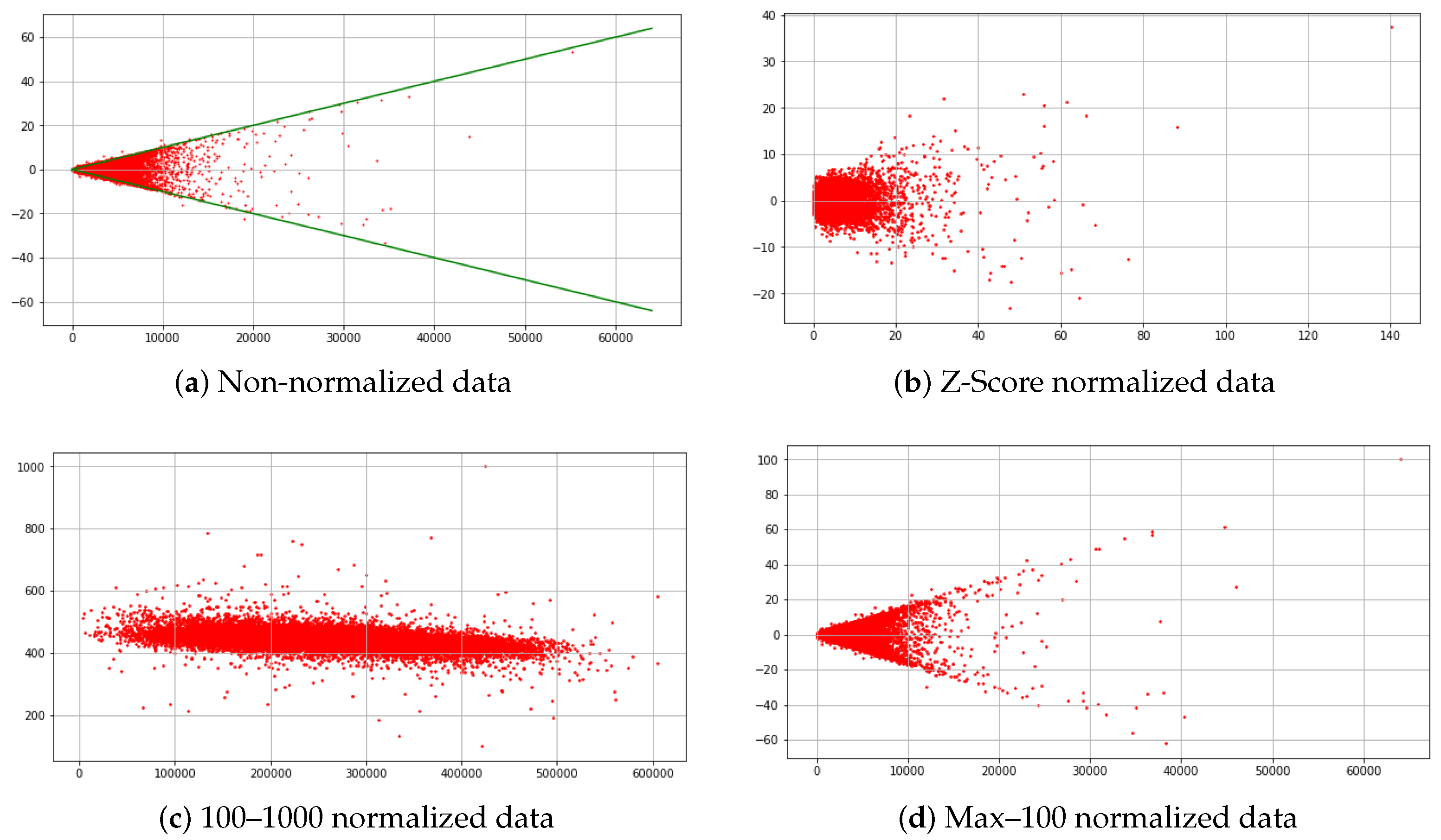
Studies have demonstrated that data-driven models, particularly neural networks, exhibit a high degree of sensitivity to fluctuations or changes in the input data [27]. Consequently, data normalization plays an important role prior to model training. We utilized the non-normalized multivariate time series as the initial data product for training our models to establish an initial baseline. The primary limitation of employing raw data is the presence of input physical parameters with varying orders of magnitude. The disparity in magnitudes between values results in a greater impact of targets with larger values on the loss compared to targets with smaller values, even when the percent error remains the same. The raw non-normalized data follows physics Ohm’s law () which constrains the range of possible values (refer Equation (6)). Figure 3a shows the raw electric field (E) data as a function of . To address this problem, we considered three data normalization techniques in addition to the raw non-normalized data: Z-Score normalization, Min–Max normalization, and Max-normalization.
3.1. Z-Score Normalization
A commonly employed normalization technique is Z-Score normalization, also known as standardization, which involves fitting the data to a Gaussian distribution. By normalizing the values, we assign them a representation based on the number of standard deviations they deviate from the mean, as defined in Equation (1). Standardization is achieved by subtracting the mean of the entire dataset and dividing it by the standard deviation. Ideally, approximately 68% of the data falls within the range of [−1, 1]. However, it should be noted that standardization does not preserve the inter-series relationships, which is a limitation of this method. Figure 3b show the data when normalized using Z-Score normalization.
3.2. Min–Max Normalization
In the deep learning community, one commonly used data normalization technique is min-max normalization, which scales the data to a range of 0 to 1. This normalization is achieved using Equation (2). We implemented a min-max normalization with the minimum value () set to 100 and the maximum value () set to 1000. Our rationale for selecting this range is driven by our proposed physics loss, which incorporates a zero as a reference point. By choosing the [100–1000] range, we ensure that the time series data values remain non-null and align with the requirements of the physics loss function. Due to the inclusion of an additional pre-processing step in min-max normalization, the maintenance of the linear physics constraint is compromised. Figure 3c illustrates that although the strict constraints in green, from the “less than” relationship, is not as apparent as depicted in Figure 3a, the data does still demonstrate a tendency to cluster together.
3.3. Max-Normalization
Max-normalization is a normalization technique where data points are expressed as a fraction of the maximum value in the time series, as demonstrated in Equation (3). This normalization approach preserves the relationship between data point pairs and the reference point (zero). By establishing a common reference point, the proposed physics-based loss ensures the invariance of data relationships. The data distribution under max-normalization is depicted in Figure 3d. The figure shows a conservative representationof the linear data constraints similar to Figure 3a.
4. Ohm’s Law Constraint
In this work, we propose a guided neural network that relies on a fundamental underlying relationship in the data, known as Ohm’s law for plasma. The law states that the electric current density in a plasma is directly proportional to the electric field and the conductivity of the plasma [2]. Equation (4) describes the relationship between the flow of electric charge and the driving force (electric field) in a plasma medium.
where J is the current vector field, is the electrical conductivity, E is the electric vector field, V is the velocity vector field, and B is the magnetic vector field. Due to the roughly equal distribution of electrons and protons in the solar wind, along with a few heavier ions, the current density is approximately zero () [28]. Therefore, we modified Equation to reflect this property, as defined in Equation (5).
A data-level limitation in our study is that while the velocity and magnetic field parameters are expressed as three vector quantities, OMNI data only provides one scalar value for the electric field. To combine all parameters into Equation (5), we relaxed the equality into an inequality property. We based this approach on the understanding that the magnitude norm of the product of three orthogonal component vectors is equal to or greater than the magnitude of each individual component vector [29]. Since Equation (5) is a vector equality, the norm of the product between the velocity field and the magnetic field must exceed the magnitude of any individual component vector, as defined in Equation (6).
where is a unit conversion constant derived from the units of the OMNI dataset features.
5. Methodology
In this work, we aim to incorporate the physics principles and constraints into the design and training process of our data driven model. To accomplish this, we propose to combine the power of neural networks in learning complex patterns and relationships with the foundational Ohm’s law for plasma. To construct a physics-constrained neural network, we utilize a loss function that penalizes the network based on violations of the Ohm’s law [30]. As discussed in Section 4, our data follows Ohm’s law for an ideal plasma that we relaxed in Equation (6).
The basic building block of a neural network is an artificial neuron, which takes multiple inputs, applies weights to each input, sums them up, and passes the result through an activation function to produce an output. The activation function is a mathematical function applied to the output of a neuron. It introduces non-linearity to the network, allowing it to learn complex patterns and make non-linear transformations to the input data [31]. Rectified Linear Unit (ReLU) is a widely used activation function that returns the input value if it is positive and zero otherwise. ReLU is mathematically defined in Equation (7). Since there is a negativity constraint in our modified Ohm’s law, we use a rectified linear unit (ReLU) as defined in Equations (8) and (9).
As we discuss in Section 6.1, we experimented with different models trained to predict different configurations of output variables, i.e., different combinations of the seven dataset features in Table 1. In the following equations, we assume that the model predicts all seven features. For other configurations, the same equations apply by replacing the non-predicted variables with their ground truth values. For example, if only the earthbound component of velocity is predicted, then . Predicted values are denoted by a ^ symbol.
We define H as a physical relation of the data. The ReLU function ensures that the predicted solar wind speed cannot have invalid values, as negative values are set to zero.
We also employed the Root Mean Square Error (RMSE) as a standard loss function for continuous values, computed as an average over all n predictions. Equation (10) shows how we compute the final loss as an aggregate value of all predicted variables’ losses, with being the set of predicted variables. For example, if all variables are predicted. To strike a balance between the two losses, we introduced a hyper-parameter denoted as . The resulting combined physics-constrained loss function is presented in Equation (11).
Deep Learning Baselines
To show the superiority of our new proposed physics loss, we tested our constraint on five deep learning baselines that we trained with our proposed combined physics-constrained loss . In this section, we outline the details of our baselines.
- Convolutional Neural Networks (CNNs): CNNs are designed to process sequential data (e.g., images and maps) that have an underlying dependence between contiguous data points [32]. Since our multivariate time series data are sequences, we used a CNN model for the predictions. Prior to training the model, we used two types of kernels. The first type of kernel is one-dimensional that performs operations on the univariate time series across the time dimension. The second kernel type is two-dimensional, which performs the operation on all the variables simultaneously. This design choice ensures that the CNN model takes into consideration both of the temporal changes in variables and the interrelationships among all the variables.
- Residual Neural Network model (ResNet): ResNet is a deep neural network architecture that addresses the challenge of training very deep networks by introducing residual connections. Residual connections allow the network to skip over certain layers, enabling the flow of information directly from earlier layers to subsequent ones. Each residual building block consists of a set of convolutional layers followed by a shortcut connection that skips one or more layers [33]. By adding these residual connections, the network can learn residual mappings instead of directly learning the desired underlying mapping. This approach helps alleviate the vanishing gradient problem and facilitates the training of deeper networks. We used the same kernels of the CNN for the ResNet model.
- RotateNet: RotateNet leverages the idea of using a convolutional neural network (CNN) as a feature extractor to capture meaningful representations from a two-dimensional matrix. It employs a combination of convolutional and fully connected layers to process the input matrices. This equips the model with additional expertise, enabling it to generate feature detectors that efficiently predict the subsequent time steps. To do so, the network constructs a neural model that acquires the ability to differentiate between distinct geometric transformations, specifically rotations, applied to the regular multivariate time series matrix [34].
- Long Short-Term Memory (LSTM): LSTM is a type of recurrent neural network architecture designed to efficiently process and learn from sequential data. LSTM networks incorporate memory cells and gates that allow them to selectively retain and forget information over extended periods [35]. This capability helps address the vanishing gradient problem and enables LSTM networks to capture and preserve relevant information from past time steps. The memory cells in LSTM networks store and update information over time by passing it through gates, including the input gate, forget gate, and output gate. These gates regulate the flow of information, allowing the network to decide which information to store, forget, or output at each time step.
- Gated Recurrent Unit (GRU): The GRU model was introduced as a variation of the LSTM architecture with a simpler structure [36]. GRU units have a simpler structure compared to LSTM, as they combine the memory and hidden state into a single unit. This simplification reduces the number of parameters and computational complexity, making GRU more computationally efficient than the LSTM. Overall, GRU provides a balance between capturing long-term dependencies and computational efficiency.
6. Experiments
6.1. Experimental Setup
In order to assess the performance of the baselines using our proposed loss function , we partitioned the data into separate training, validation, and testing sets. We then utilized the measure, as described in Equation (12), to evaluate their performance. Additionally, we conducted a grid search over the architectures and hyperparameters of the baseline models before training the baseline models. This search was performed on data divided into a 60/30/10 split, with the first partition as training data, the second as validation data, and the final partition as testing data. After seven hundred epochs of training, each network was assessed on the testing data. To fine-tune the models’ hyperparameters, we repeated this process three times.
Since metric is defined on the range, there are possibilities of extremely large negative numbers that inhibit the making of coherent linear graphs. To address this issue, we normalized the values into a range of (−1, 1], and we introduce a transformation equation: , where y is the new plotted height and z is the original value.
To show the superiority of our proposed physics loss function, we trained the deep learning baselines with the new loss and the traditional loss. We conducted experiments involving various combinations of predictor and target values. We defined three prediction groups: (1) all the seven available components in Table 1 (i.e., ), (2) the 3-vector of velocity v, and (3) the 3-vector of the magnetic field B. We also selected four categories of outputs: (1) all the seven available components in Table 1, (2) the 3-vector of velocity v, (3) the 3-vector of the magnetic field B, and (4) the earthbound component of velocity . In total, we performed a total of 1200 individual training and testing cycles, where each of the five baselines were trained on all possible combinations of four predictors, three targets, two loss functions, and repeated 10 times. The computations were performed on four NVIDIA RTX A4000 GPUs.
6.2. Experimental Evaluation
Our experimental evaluation is divided in two folds. First, we assess the results on a fixed length of the time series input data to determine the effect of our new physics loss. Then, we perform sequence analysis experiments to understand the impact of dimensionality on our prediction results.
Figure 4a shows the violin plot of the normalized value of all the models when trained with physics loss and without physics loss, with respect to the input predictor variables. The left part of the violin plots shows the distribution of the normalized achieved by all the five baseline models when trained on physics loss, and the right part of the violin plot shows the distribution of the normalized achieved by all the five baseline models when the physics loss is not used. The first observation we note is that the models achieve the best results when all the input variables (i.e., , , , v, and x) are used for the prediction. The second observation we note is that there is a significant discrepancy between the two distributions of normalized when the networks use the physics loss and when they do not. This suggests that using all the OMNI predictor variables benefit the prediction task regardless of the target variable. Figure 4b shows the violin plot of the normalized value of all the models when trained with physics loss and without physics loss, with respect to the target variables. It is important to note that the baselines achieve better values when the target variable is . The baselines shows a clear improvement when using a physics loss and predicting the x component of the solar wind velocity (i.e., ). This observation suggests that when the neural networks are trained to predict a smaller set of output variables, the final linear layers of each network can capture and retain more pertinent information related to the desired target variable. In contrast, when the baselines predict , or v, the latent space is distributed across the seven or three regression targets, leading to a more intricate flow of relevant information. The multi-target (i.e., , or v) prediction achieves lower scores. Figure 5 shows the modified values achieved by each of the five networks when trained with the physics loss and without physics loss . The dashed line represents the reference line that serves as a baseline for comparison between the same model when trained with two different losses (i.e., versus ). The plots show that for all the five baselines, the number of physics loss wins encompasses the number of losses (and ties). This suggests that all the models benefits from the usage of physics loss regardless of the targets and predictor variables.
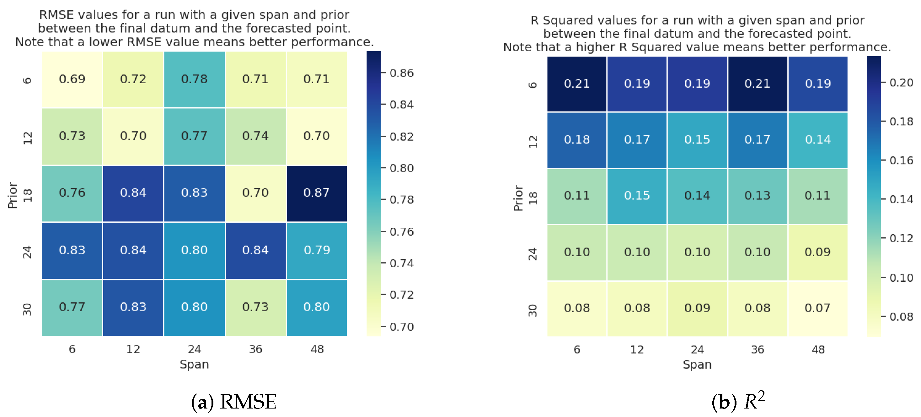
Our second set of experiments aim to determine the optimal input dimensionality prior to the prediction time for the baseline models that uses our proposed physics loss. To achieve this, we define two variables (prior and span) that we change to monitor the prediction impact. The prior variable signifies the number of hours prior to the solar wind occurrence. We selected five different values of priors: 6, 12, 18, 24, and 30 h. The span signifies the observation period, in other words, the number of hours we observe the OMNI features (defined in Table 1). We selected five different spans: 6, 12, 24, 36 and 48 h. We trained each baseline on all the 25 (5 × 5) possible combinations of span and prior using three-fold cross validation and repeated the process 10 times. We report the average of ten runs for each baseline model. Figure 6, Figure 7, Figure 8 and Figure 9 show the RMSE and metric values for each baseline model. We note that for the case of GRU network (refer Figure 6), the RMSE error decreases as the window increases, which is intuitive. However, the relative stability of the error shows that the have a low impact on the prediction accuracy. The values of the GRU network show that the baseline is estimating predictions close to the mean solar wind speed, which results in a poor performance. It is important to note that the variation in RMSE values across orders of magnitude is primarily attributed to differing data normalizations adopted by distinct networks, resulting in predictions spanning dissimilar numerical ranges.
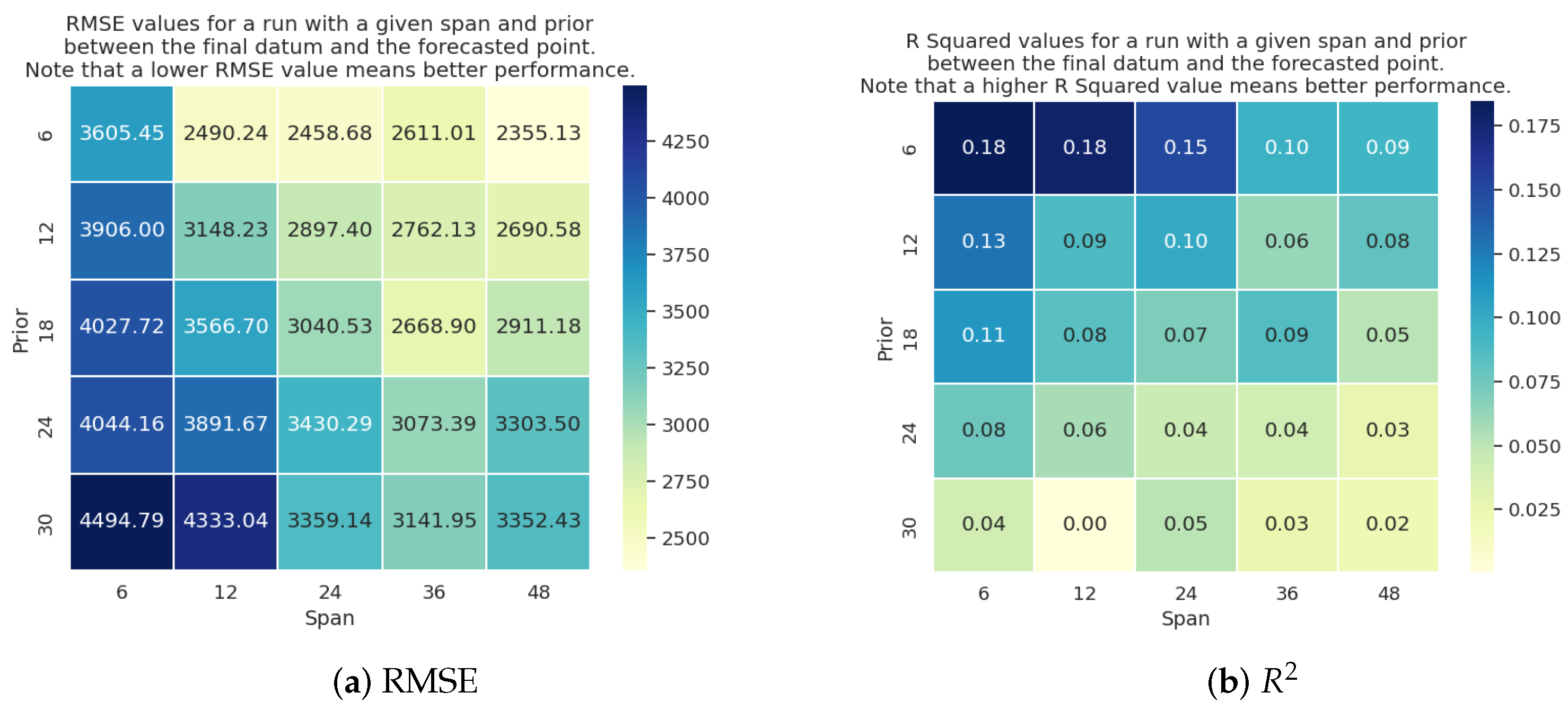
On the other hand, the LSTM results, shown in Figure 7, shows that the prediction results are variant over different priors. The LSTM model achieves better results when using shorter priors and was resilient against changes in span windows. This is due to the design of the LSTM that memorizes information for an indeterminate amount of steps which makes it better equipped to adapt the predictions given different length of spans. For the case of ResNet, RotateNet, and CNN, as shown in Figure 8, Figure 9 and Figure 10, respectively, the models achieve optimal performance with the shortest prior and longest span (i.e., prior = 6 h and span = 48 h).
7. Case Study: Solar Cycles
In this section, we study the effect of the proposed physics loss when training the deep learning baselines on the data of solar cycles 22, 23, and 24. To achieve this, we divide the data into separate solar cycles instead of random shuffling. We test the solar cycle effect by training the baselines on (i.e., all seven parameters) as predictors and as target values. We then select the best normalization and loss parameters that produce the best results. The optimal parameters are:
- LSTM: No physics loss () and input data Z-normalized.
- CNN: Physics loss () with a weight ( = 0.3), and input data normalized from 100 to 1000.
- ResNet: Physics loss () with a weight ( = 0.0001), and input data normalized using max-normalization.
- RotateNet: Physics loss () with a weight ( = 0.003), and input data normalized from 100 to 1000.
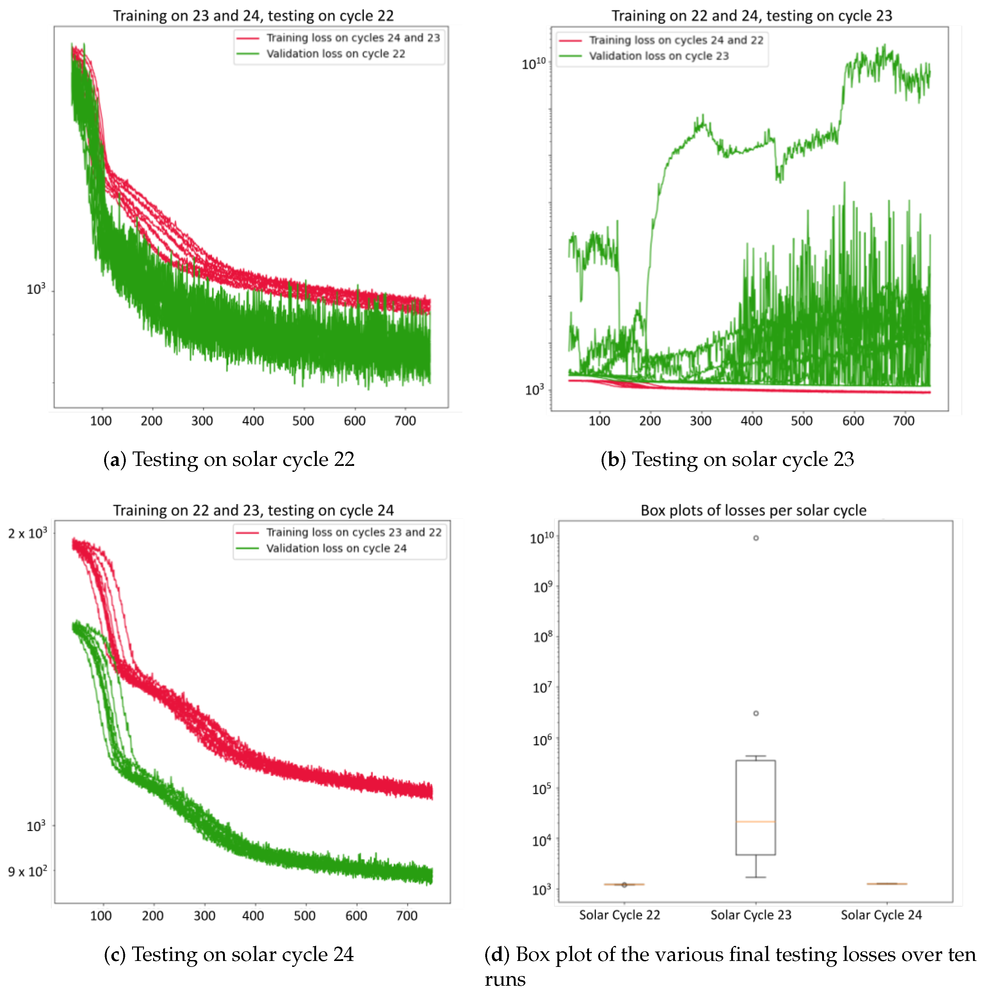
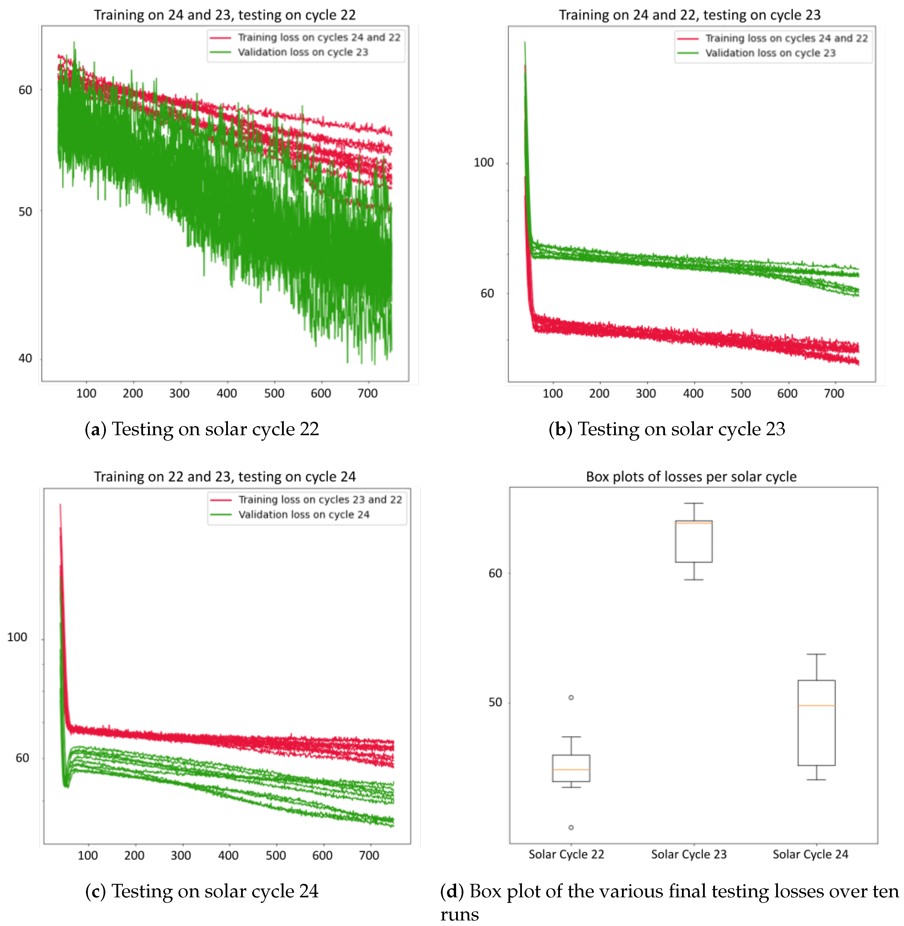
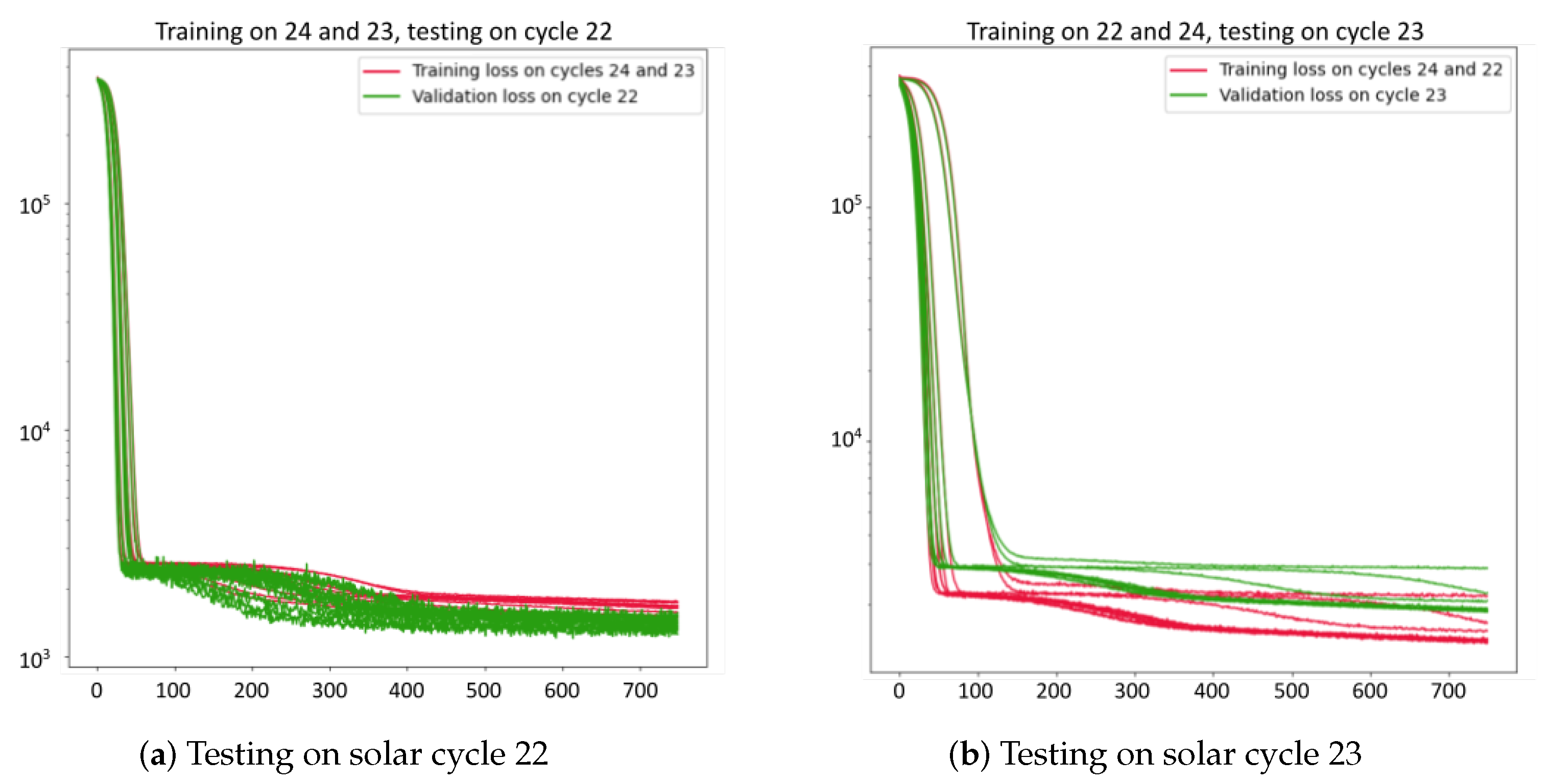
Figure 11, Figure 12, Figure 13, Figure 14 and Figure 15 show the baseline learning curves using the testing and training set when trained on two solar cycles and tested on one solar cycle. An ideal neural network learning curve demonstrates a decreasing training loss, indicating effective learning and error reduction. The validation loss should also decrease initially, signifying good generalization to unseen data. Also, a small gap between the training and validation loss, and consistency across runs are characteristics of an ideal learning curve. The aforementioned criteria are satisfied when the networks are trained on solar cycles 22 and 24 and tested on solar cycle 23. In contrast, when the networks are trained on solar cycles 23 and 24 and tested on 22, or trained on 22 and 23 and tested on 24, they achieve higher testing accuracies compared to their respective training accuracies. The main reason of the abnormal convergence comes from the inherent data characteristics. Our assumption is that solar cycles 22 and 24 have a different data distribution than the other solar cycles used for training. Therefore, the training data, when testing on solar cycles 22 and 23, does not provide a representative sample that ensure that the model learns from diverse and relevant examples that accurately represent the underlying data distribution. To validate our assumption, we plotted the kernel distribution of all the seven prediction variables across the three solar cycles. The kernel distributions, as illustrated in Figure 16, reveal noticeable variations throughout solar cycles. Out of the seven variables shown, solar cycle 23 has both the maximum and the minimum values for five of the predictor variables. This suggests that the baseline methods that are not trained on solar cycle 23 are not exposed to extreme values, resulting in relatively low prediction accuracy. Similarly, solar cycle 22 kernel distributions, namely the distribution of and , display values that fall outside the the normal distribution of solar cycles 23 and 24. We note that solar cycle 24 generally follows the same patterns as solar cycle 23, and to a lesser extent 22. Therefore, training the baselines on solar cycle 23 supported with cycle 22 data, provides a more complete sampling of the input space than any other combination.
8. Conclusions
In this paper, we propose an adjusted Ohm’s law inequality that we used for developing a new physics loss to guide deep learning models for the task of solar wind prediction. We demonstrate the variability of the proposed physics-informed loss across five deep learning baseline models. Additionally, we investigate the impact of training the models on different solar cycles on their performance. This work represents the first effort to forecast solar wind by integrating data-driven methods with physics constraints. Our findings support our hypothesis that physics loss helps fine-tune model predictions by eliminating the possibility of producing prediction that violates the Ohm’s law constraint. As a future direction to this work, we would like to explore the inclusion of physics models (e.g., WSA-ENLIL) forecasts as an input to produce a hybrid physics-informed model. Finally, we recognize the potential limitations associated with utilizing OMNI data for magnetic field measurements, in particular as the distance between the OMNI spacecraft from the Sun-Earth line increases [37,38]. Moving forward, we plan to explore the use of direct measurements from the ACE satellite to further validate and enhance the robustness of our findings.
Author Contributions
Conceptualization, R.J.; methodology, R.J. and O.B.; software, R.J.; validation, R.J. and O.B.; formal analysis, R.J.; investigation, R.J.; data curation, R.J.; writing—original draft preparation, R.J. and S.F.B.; writing—review and editing, R.J., O.B. and S.M.H.; visualization, R.J.; supervision, O.B.; project administration, S.F.B.; funding acquisition, S.F.B. and S.M.H. All authors have read and agreed to the published version of the manuscript.
Funding
This project has been supported in part by funding from GEO Directorate under NSF awards #2204363, #2240022, and #2301397 and the CISE Directorate under NSF award #2305781.
Data Availability Statement
The NASA OMNI dataset is available via [https://omniweb.gsfc.nasa.gov/ (accessed on 18 April 2024)]. The experimental results were generated using Python 3.6, which can be found at [https://sites.google.com/view/solarwindprediction/ (accessed on 18 April 2024)]. Our code makes use of several open source libraries, including sktime [39], scikit-learn [40], matplotlib [41], and NumPy [42].
Acknowledgments
The authors acknowledge the use of ChatGPT (GPT-3.5) to rephrase sentences and improve the writing style of the manuscript, including the Section 5.
Conflicts of Interest
The authors declare no conflict of interest.
References
- Eastwood, J.; Biffis, E.; Hapgood, M.; Green, L.; Bisi, M.; Bentley, R.; Wicks, R.; McKinnell, L.A.; Gibbs, M.; Burnett, C. The Economic Impact of Space Weather: Where Do We Stand? Risk Anal. 2017, 37, 206–218. [Google Scholar] [CrossRef]
- Boozer, A.H. Ohm’s law for mean magnetic fields. J. Plasma Phys. 1986, 35, 133–139. [Google Scholar] [CrossRef]
- Martin, S. Solar Winds Travelling at 300 km per second to Hit Earth Today. 2021. Available online: https://www.express.co.uk/news/science/1449974/solar-winds-space-weather-forecast-sunspot-solar-storm-aurora-evg (accessed on 1 May 2022).
- de La Baume Pluvinel, A.; Baldet, F. Spectrum of comet morehouse (1908 c). Astrophys. J. 1911, 34, 89. [Google Scholar] [CrossRef]
- Pizzo, V. Wang-Sheeley-Arge-Enlil cone model transitions to operations. Space Weather 2011, 9. [Google Scholar] [CrossRef]
- Rotter, T.; Veronig, A.; Temmer, M.; Vršnak, B. Relation between coronal hole areas on the Sun and the solar wind parameters at 1 AU. Sol. Phys. 2012, 281, 793–813. [Google Scholar] [CrossRef]
- Feng, X. Current Status of MHD Simulations for Space Weather. In Magnetohydrodynamic Modeling of the Solar Corona and Heliosphere; Springer: Singapore, 2020; pp. 1–123. [Google Scholar] [CrossRef]
- Baker, D.N.; Poh, G.; Odstrcil, D.; Arge, C.N.; Benna, M.; Johnson, C.L.; Korth, H.; Gershman, D.J.; Ho, G.C.; McClintock, W.E.; et al. Solar wind forcing at Mercury: WSA-ENLIL model results. J. Geophys. Res. Space Phys. 2013, 118, 45–57. [Google Scholar] [CrossRef]
- Owens, M.; Lang, M.; Barnard, L.; Riley, P.; Ben-Nun, M.; Scott, C.J.; Lockwood, M.; Reiss, M.A.; Arge, C.N.; Gonzi, S. A Computationally Efficient, Time-Dependent Model of the Solar Wind for Use as a Surrogate to Three-Dimensional Numerical Magnetohydrodynamic Simulations. Sol. Phys. 2020, 295, 43. [Google Scholar] [CrossRef]
- Shugai, Y.S. Analysis of Quasistationary Solar Wind Stream Forecasts for 2010–2019. Russ. Meteorol. Hydrol. 2021, 46, 172–178. [Google Scholar] [CrossRef]
- Yang, Y.; Shen, F. Three-Dimensional MHD Modeling of Interplanetary Solar Wind Using Self-Consistent Boundary Condition Obtained from Multiple Observations and Machine Learning. Universe 2021, 7, 371. [Google Scholar] [CrossRef]
- Luo, B.; Zhong, Q.; Liu, S.; Gong, J. A New Forecasting Index for Solar Wind Velocity Based on EIT 284 Å Observations. Sol. Phys. 2008, 250, 159–170. [Google Scholar] [CrossRef]
- Upendran, V.; Cheung, M.C.; Hanasoge, S.; Krishnamurthi, G. Solar wind prediction using deep learning. Space Weather 2020, 18, e2020SW002478. [Google Scholar] [CrossRef]
- Yang, Y.; Shen, F. Modeling the Global Distribution of Solar Wind Parameters on the Source Surface Using Multiple Observations and the Artificial Neural Network Technique. Sol. Phys. 2019, 294, 111. [Google Scholar] [CrossRef]
- Raju, H.; Das, S. CNN-Based Deep Learning Model for Solar Wind Forecasting. Sol. Phys. 2021, 296, 134. [Google Scholar] [CrossRef]
- Leitner, M.; Farrugia, C.; Vörös, Z. Change of solar wind quasi-invariant in solar cycle 23—Analysis of PDFs. J. Atmos. Sol.-Terr. Phys. 2011, 73, 290–293. [Google Scholar] [CrossRef]
- Sun, Y.; Xie, Z.; Chen, Y.; Huang, X.; Hu, Q. Solar Wind Speed Prediction With Two-Dimensional Attention Mechanism. Space Weather 2021, 19, e2020SW002707. [Google Scholar] [CrossRef]
- van der Schaaf, A.; Xu, C.J.; van Luijk, P.; van’t Veld, A.A.; Langendijk, J.A.; Schilstra, C. Multivariate modeling of complications with data driven variable selection: Guarding against overfitting and effects of data set size. Radiother. Oncol. 2012, 105, 115–121. [Google Scholar] [CrossRef] [PubMed]
- Johnson, R.; Boubrahimi, S.F.; Bahri, O.; Hamdi, S.M. Physics-Informed Neural Networks For Solar Wind Prediction. In Lecture Notes in Computer Science; Springer Nature: Cham, Switzerland, 2023. [Google Scholar]
- Shin, Y.; Darbon, J.; Karniadakis, G.E. On the convergence of physics informed neural networks for linear second-order elliptic and parabolic type PDEs. Commun. Comput. Phys. 2020, 28, 2042–2074. [Google Scholar] [CrossRef]
- Mishra, S.; Molinaro, R. Estimates on the generalization error of physics-informed neural networks for approximating a class of inverse problems for PDEs. IMA J. Numer. Anal. 2022, 42, 981–1022. [Google Scholar] [CrossRef]
- Zhao, J.; Feng, X.; Xiang, C.; Jiang, C. A mutually embedded perception model for solar corona. Mon. Not. R. Astron. Soc. 2023, 523, 1577–1590. [Google Scholar] [CrossRef]
- Jarolim, R.; Thalmann, J.K.; Veronig, A.M.; Podladchikova, T. Probing the solar coronal magnetic field with physics-informed neural networks. Nat. Astron. 2023, 7, 1171–1179. [Google Scholar] [CrossRef]
- Wilkinson, M.D.; Dumontier, M.; Aalbersberg, I.J.; Appleton, G.; Axton, M.; Baak, A.; Blomberg, N.; Boiten, J.W.; da Silva Santos, L.B.; Bourne, P.E.; et al. The FAIR Guiding Principles for scientific data management and stewardship. Sci. Data 2016, 3, 1–9. [Google Scholar] [CrossRef]
- Papitashvili, N.; Bilitza, D.; King, J. OMNI: A description of near-Earth solar wind environment. In Proceedings of the 40th COSPAR Scientific Assembly, Moscow, Russia, 2–10 August 2014; Volume 40. [Google Scholar]
- Mukai, T.; Machida, S.; Saito, Y.; Hirahara, M.; Terasawa, T.; Kaya, N.; Obara, T.; Ejiri, M.; Nishida, A. The Low Energy Particle (LEP) Experiment onboard the GEOTAIL Satellite. J. Geomagn. Geoelectr. 1994, 46, 669–692. [Google Scholar] [CrossRef]
- Bartlett, P.L.; Foster, D.J.; Telgarsky, M. Spectrally-Normalized Margin Bounds for Neural Networks. In Proceedings of the 31st International Conference on Neural Information Processing Systems (NIPS’17), Red Hook, NY, USA, 4–9 December 2017; pp. 6241–6250. [Google Scholar]
- Padhye, N.; Smith, C.; Matthaeus, W. Distribution of magnetic field components in the solar wind plasma. J. Geophys. Res. Space Phys. 2001, 106, 18635–18650. [Google Scholar] [CrossRef]
- Bresler, A.; Joshi, G.; Marcuvitz, N. Orthogonality properties for modes in passive and active uniform wave guides. J. Appl. Phys. 1958, 29, 794–799. [Google Scholar] [CrossRef]
- Karpatne, A.; Watkins, W.; Read, J.S.; Kumar, V. Physics-guided Neural Networks (PGNN): An Application in Lake Temperature Modeling. arXiv 2017, arXiv:1710.11431. [Google Scholar]
- Sharma, S.; Sharma, S.; Athaiya, A. Activation functions in neural networks. Towards Data Sci 2017, 6, 310–316. [Google Scholar] [CrossRef]
- Albawi, S.; Mohammed, T.A.; Al-Zawi, S. Understanding of a convolutional neural network. In Proceedings of the 2017 International Conference on Engineering and Technology (ICET), Antalya, Turkey, 21–23 August 2017; pp. 1–6. [Google Scholar] [CrossRef]
- Li, S.; Jiao, J.; Han, Y.; Weissman, T. Demystifying resnet. arXiv 2016, arXiv:1611.01186. [Google Scholar]
- Golan, I.; El-Yaniv, R. Deep anomaly detection using geometric transformations. In Proceedings of the Advances in Neural Information Processing Systems 31: Annual Conference on Neural Information Processing Systems 2018 (NeurIPS 2018), Montréal, QC, Canada, 3–8 December 2018; Volume 31. [Google Scholar]
- Breuel, T.M. Benchmarking of LSTM networks. arXiv 2015, arXiv:1508.02774. [Google Scholar]
- Cho, K.; van Merriënboer, B.; Bahdanau, D.; Bengio, Y. On the Properties of Neural Machine Translation: Encoder–Decoder Approaches. In Proceedings of the SSST-8, Eighth Workshop on Syntax, Semantics and Structure in Statistical Translation, Doha, Qatar, 25 October 2014; Wu, D., Carpuat, M., Carreras, X., Vecchi, E.M., Eds.; pp. 103–111. [Google Scholar] [CrossRef]
- Case, N.A.; Wild, J.A. A statistical comparison of solar wind propagation delays derived from multispacecraft techniques. J. Geophys. Res. Space Phys. 2012, 117, 2101. [Google Scholar] [CrossRef]
- Vokhmyanin, M.V.; Stepanov, N.A.; Sergeev, V.A. On the Evaluation of Data Quality in the OMNI Interplanetary Magnetic Field Database. Space Weather 2019, 17, 476–486. [Google Scholar] [CrossRef]
- Löning, M.; Bagnall, A.; Ganesh, S.; Kazakov, V.; Lines, J.; Király, F.J. sktime: A unified interface for machine learning with time series. arXiv 2019, arXiv:1909.07872. [Google Scholar]
- Kramer, O.; Kramer, O. Scikit-learn. In Machine Learning for Evolution Strategies; Springer: Cham, Switzerland, 2016; pp. 45–53. [Google Scholar]
- Bisong, E.; Bisong, E. Matplotlib and seaborn. In Building Machine Learning and Deep Learning Models on Google Cloud Platform: A Comprehensive Guide for Beginners; Springer: Cham, Switzerland, 2019; pp. 151–165. [Google Scholar] [CrossRef]
- Harris, C.R.; Millman, K.J.; van der Walt, S.J.; Gommers, R.; Virtanen, P.; Cournapeau, D.; Wieser, E.; Taylor, J.; Berg, S.; Smith, N.J.; et al. Array programming with NumPy. Nature 2020, 585, 357–362. [Google Scholar] [CrossRef] [PubMed]
Figure 1.
Solar wind traveling to Earth at the speed of 300 km per second (Image Courteousy from [3]).
Figure 1.
Solar wind traveling to Earth at the speed of 300 km per second (Image Courteousy from [3]).

Figure 2.
OMNI time series data snapshot for the year 1992.

Figure 3.
Scatterplots of E as a function of under (a) no data normalization, (b) standardization, (c) min-max normalization, and (d) max-100 normalization. (The green lines show the relationship which follows the adapted Ohm’s Law).
Figure 3.
Scatterplots of E as a function of under (a) no data normalization, (b) standardization, (c) min-max normalization, and (d) max-100 normalization. (The green lines show the relationship which follows the adapted Ohm’s Law).

Figure 4.
Distribution of modified results of the five baseline models using physics loss and without physics loss (a) per input predictor variables, and (b) per target variable.
Figure 4.
Distribution of modified results of the five baseline models using physics loss and without physics loss (a) per input predictor variables, and (b) per target variable.

Figure 5.
Modified values of the five models when trained with physics loss and without physics loss .
Figure 5.
Modified values of the five models when trained with physics loss and without physics loss .

Figure 6.
Heatmaps of GRU model performance trained with different priors and spans using (a) RMSE and (b) metrics.
Figure 6.
Heatmaps of GRU model performance trained with different priors and spans using (a) RMSE and (b) metrics.

Figure 7.
Heatmaps of LSTM model performance trained with different priors and spans using (a) RMSE and (b) metrics.
Figure 7.
Heatmaps of LSTM model performance trained with different priors and spans using (a) RMSE and (b) metrics.

Figure 8.
Heatmaps of ResNet model performance trained with different priors and spans using (a) RMSE and (b) metrics.
Figure 8.
Heatmaps of ResNet model performance trained with different priors and spans using (a) RMSE and (b) metrics.

Figure 9.
Heatmaps of RotateNet model performance trained with different priors and spans using (a) RMSE and (b) metrics.
Figure 9.
Heatmaps of RotateNet model performance trained with different priors and spans using (a) RMSE and (b) metrics.

Figure 10.
Heatmaps of CNN model performance trained with different priors and spans using (a) RMSE and (b) metrics.
Figure 10.
Heatmaps of CNN model performance trained with different priors and spans using (a) RMSE and (b) metrics.

Figure 11.
Learning curve of the LSTM model when (a) trained on solar cycles 23 and 24 and tested on 22, (b) trained on solar cycles 22 and 24 and tested on 23, (c) trained on solar cycles 22 and 23 and tested on 24, and (d) boxplot of the losses across the 10 runs.
Figure 11.
Learning curve of the LSTM model when (a) trained on solar cycles 23 and 24 and tested on 22, (b) trained on solar cycles 22 and 24 and tested on 23, (c) trained on solar cycles 22 and 23 and tested on 24, and (d) boxplot of the losses across the 10 runs.

Figure 12.
Learning curve of the CNN model when (a) trained on solar cycles 23 and 24 and tested on 22, (b) trained on solar cycles 22 and 24 and tested on 23, (c) trained on solar cycles 22 and 23 and tested on 24, and (d) boxplot of the losses across the 10 runs.
Figure 12.
Learning curve of the CNN model when (a) trained on solar cycles 23 and 24 and tested on 22, (b) trained on solar cycles 22 and 24 and tested on 23, (c) trained on solar cycles 22 and 23 and tested on 24, and (d) boxplot of the losses across the 10 runs.


Figure 13.
Learning curve of the ResNet model when (a) trained on solar cycles 23 and 24 and tested on 22, (b) trained on solar cycles 22 and 24 and tested on 23, (c) trained on solar cycles 22 and 23 and tested on 24, and (d) boxplot of the losses across the 10 runs.
Figure 13.
Learning curve of the ResNet model when (a) trained on solar cycles 23 and 24 and tested on 22, (b) trained on solar cycles 22 and 24 and tested on 23, (c) trained on solar cycles 22 and 23 and tested on 24, and (d) boxplot of the losses across the 10 runs.

Figure 14.
Learning curve of the GRU model when (a) trained on solar cycles 23 and 24 and tested on 22, (b) trained on solar cycles 22 and 24 and tested on 23, (c) trained on solar cycles 22 and 23 and tested on 24, and (d) boxplot of the losses across the 10 runs.
Figure 14.
Learning curve of the GRU model when (a) trained on solar cycles 23 and 24 and tested on 22, (b) trained on solar cycles 22 and 24 and tested on 23, (c) trained on solar cycles 22 and 23 and tested on 24, and (d) boxplot of the losses across the 10 runs.

Figure 15.
Learning curve of the RotateNet model when (a) trained on solar cycles 23 and 24 and tested on 22, (b) trained on solar cycles 22 and 24 and tested on 23, (c) trained on solar cycles 22 and 23 and tested on 24, and (d) boxplot of the losses across the 10 runs.
Figure 15.
Learning curve of the RotateNet model when (a) trained on solar cycles 23 and 24 and tested on 22, (b) trained on solar cycles 22 and 24 and tested on 23, (c) trained on solar cycles 22 and 23 and tested on 24, and (d) boxplot of the losses across the 10 runs.


Figure 16.
Kernel density plots of the seven predictor variables (solar cycles 22, 23, and 24).


Table 1.
OMNI features and metadata.
| Feature | Unit | Description |
|---|---|---|
| E | mV/m | Electric field |
| km/s | X component of the velocity | |
| km/s | Y component of the velocity | |
| km/s | Z component of the velocity | |
| nT | X component of the magnetic field | |
| nT | Y component of the magnetic field | |
| nT | Z component of the magnetic field |
Disclaimer/Publisher’s Note: The statements, opinions and data contained in all publications are solely those of the individual author(s) and contributor(s) and not of MDPI and/or the editor(s). MDPI and/or the editor(s) disclaim responsibility for any injury to people or property resulting from any ideas, methods, instructions or products referred to in the content. |
© 2024 by the authors. Licensee MDPI, Basel, Switzerland. This article is an open access article distributed under the terms and conditions of the Creative Commons Attribution (CC BY) license (https://creativecommons.org/licenses/by/4.0/).
Share and Cite
MDPI and ACS Style
Johnson, R.; Filali Boubrahimi, S.; Bahri, O.; Hamdi, S.M. Combining Empirical and Physics-Based Models for Solar Wind Prediction. Universe 2024, 10, 191. https://doi.org/10.3390/universe10050191
AMA Style
Johnson R, Filali Boubrahimi S, Bahri O, Hamdi SM. Combining Empirical and Physics-Based Models for Solar Wind Prediction. Universe. 2024; 10(5):191. https://doi.org/10.3390/universe10050191
Chicago/Turabian StyleJohnson, Rob, Soukaina Filali Boubrahimi, Omar Bahri, and Shah Muhammad Hamdi. 2024. "Combining Empirical and Physics-Based Models for Solar Wind Prediction" Universe 10, no. 5: 191. https://doi.org/10.3390/universe10050191
Note that from the first issue of 2016, this journal uses article numbers instead of page numbers. See further details here.