Spin-Field Correspondence

Institute of Physics, Jagiellonian University, ul. ojasiewicza 11, 30-348 Kraków, Poland
Universe 2017, 3(2), 29; https://doi.org/10.3390/universe3020029
Submission received: 4 January 2017
/
Revised: 15 March 2017
/
Accepted: 21 March 2017
/
Published: 23 March 2017
(This article belongs to the Special Issue Varying Constants and Fundamental Cosmology)
Abstract
:In the recent article Phys. Lett. B 2016, 759, 424–429, a new class of field theories called Nonlinear Field Space Theory was proposed. In this approach, the standard field theories are considered as linear approximations to some more general theories characterized by nonlinear field phase spaces. The case of spherical geometry is especially interesting due to its relation with the spin physics. Here, we explore this possibility, showing that classical scalar field theory with such a field space can be viewed as a perturbation of a continuous spin system. In this picture, the spin precession and the scalar field excitations are dual descriptions of the same physics. The duality is studied in the example of the Heisenberg model. It is shown that the Heisenberg model coupled to a magnetic field leads to a non-relativistic scalar field theory, characterized by quadratic dispersion relation. Finally, on the basis of analysis of the relation between the spin phase space and the scalar field theory, we propose the Spin-Field correspondence between the known types of fields and the corresponding spin systems.
1. Introduction
The phase space of a classical spin is a two-sphere, (see e.g., [1]). Because the phase space is a symplectic manifold, it has to be equipped with the closed symplectic form , for which the natural choice is the area two-form. Using the standard spherical coordinates , the symplectic form can be written as . The J is a constant introduced due to dimensional reasons, equal to the absolute value of the spin (angular momentum). Except for the poles , the symplectic form is well defined and invertible, allowing for determination of the Poisson tensor , and then we can define the Poisson bracket . The Hamilton equation can then be defined as , where f is a phase space function and H is the Hamiltonian.
It turns out that instead of using the spherical coordinates , it is useful to apply another local parametrization of sphere. Let us consider the following change of coordinates:
where q and p are our new phase space variables and and are constants introduced due to dimensional reasons. Using the new variables, the symplectic form can be written as , where we fixed . The last condition guarantees that for small values of p (), the symplectic form reduces to the Darboux form . Employing the new variables, the Poisson bracket related to can now be written as:
The variables, similarly to the pair, are defined only locally. It is, however, often convenient to work with the globally defined functions. The most important example of such functions are components of the angular momentum vector , which can be defined as follows:
together with the condition . Here, for the purpose of our further analysis, the leading order expansions have been included. In the atomic physics, a magnetic moment couples to an external magnetic field via the vector . In such a case, the Hamiltonian of the interaction is
where is the value of the magnetic moment, which can be both positive and negative. Based on (7), together with the fact that the components satisfy the algebra bracket , one can write the Hamilton equation for the vector in the following form:
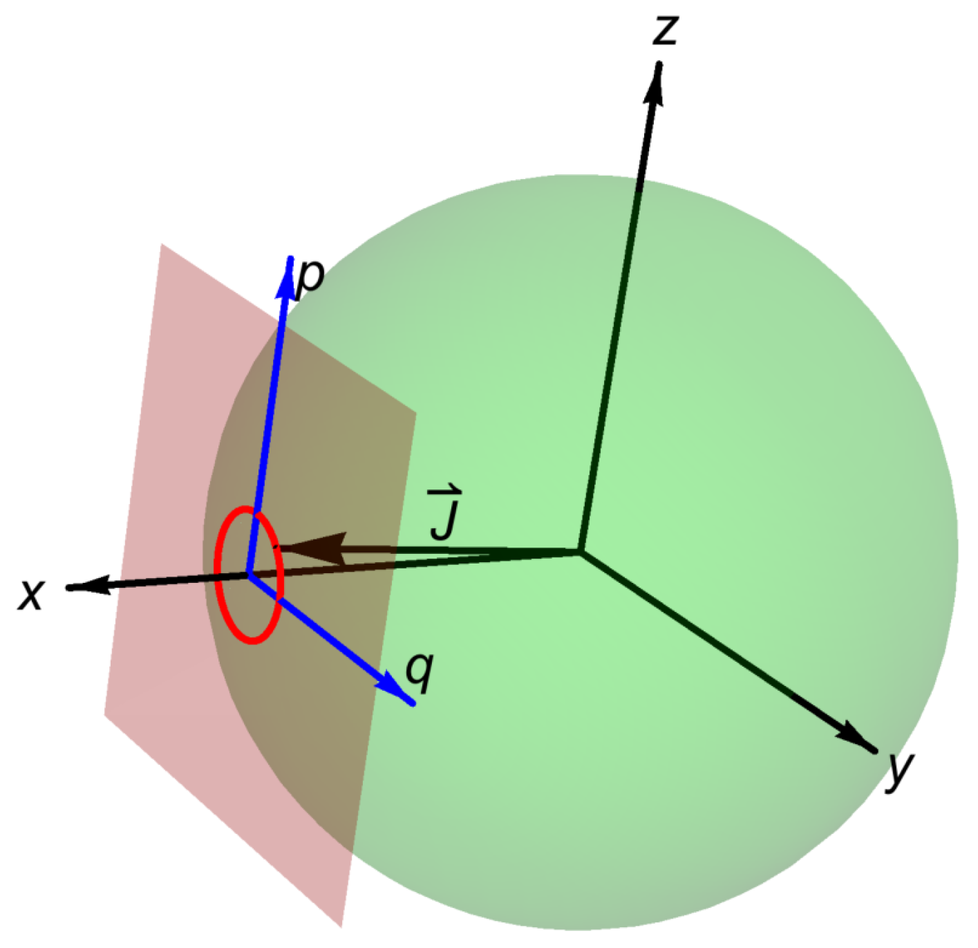
Equation (8) describes the precession of a magnetic moment in a constant magnetic field. The process plays a crucial role in our construction. Firstly, let us notice that the arrow of the vector goes around a circle (see Figure 1). Secondly, suppose that the precession angle (angle between the and vectors) is small. Then, let us make use of the new variables and direct the vector through the origin of the coordinate system (i.e., along the x axis).
One can now easily conclude that the precession of the vector corresponds to a circle in the phase space. The precession (for small precession angles) is, therefore, described by a harmonic oscillator. In order to see this explicitly, let us fix so that precession takes place around the origin of the coordinate system. Then, for small spin displacements from the equilibrium point, the Hamiltonian (7) can be written as
where we defined the constants such that and . The constant energy trajectory is, in general, an ellipse in the variables or a circle if the variables are appropriately rescaled, namely if the pair is considered.
The picture can now be generalized to the area of field theory. For this purpose, let us consider a continuous spin distribution, which may be viewed as an approximated description of some discrete spin systems studied experimentally. Then, at any space point, the following identification can be performed:
The continuous spin system is, therefore, in correspondence with the scalar field theory with the spherical field phase space. This is basically because the dimension of the scalar field phase space at any point is equal to the dimension of the spin phase space:
Depending on the particular form of the interactions between the spins, different types of the field theories with the bounded field spaces can be reconstructed. In what follows, we consider the Heisenberg model of the spin system and find what is the field theoretical counterpart in such a case.
2. The Heisenberg Model
The Heisenberg model with an external magnetic field can be defined by the following Hamiltonian:
where and are real-valued coupling constants and the first sum is performed over the nearest neighbors. The indices are labeling different spins (not the spin vector components) distributed on a regular three-dimensional lattice. In the physical picture of ferromagnets, the spins are accompanied by magnetic moments. Here, the 3D spin lattice is considered. However, an analogous analysis can be performed in case of other dimensions of the spin lattice (e.g., 1D or 2D). The Spin-Field Correspondence (at least for the case of a scalar field considered here) does not rely on the dimensionality of the spin lattice of the dual condensed matter system. The only restriction on dimensionality concerns the phase space, which has to be dimensionally even dimensional, such as the two dimensional case for a system with a single spin per point.
The discrete spin system described by the Heisenberg model (13) can be approximated by continuous spin distribution. In such a limit, the spin labels i are replaced by the position vector and, neglecting the higher-order derivatives, the corresponding continuous version of the Hamiltonian (13) can be written as:
together with the condition . The sign change of the first factor with respect to Expression (13) appears to be a consequence of the integration by parts. Here, and are new coupling constants determined by , and a lattice spacing parameter.
Let us now choose the direction of the vector along the x axis. In this way, the set of field variables, Equations (10) and (11), discussed in the previous section can be introduced. Additionally, it is worth mentioning here that Expression (14), interpreted not as a Hamiltonian but as a Lagrangian, gives us a certain non-linear sigma model [2].
Using relations Equations (4) and (5) together with Equations (10) and (11), we find that the scalar field Hamiltonian density resulting from (14) is up to the quadratic terms:
where we fixed the first three terms to have the standard form. This leads to the following relations between the parameters:
where we also used the condition coming from the small field values limit of the symplectic form. Substantially, J and M can be treated as two independent parameters. However, then we have to keep in mind that the coupling constants and may vary as functions of J and M. On the other hand, one may assume that is fixed, and then . Actually, the presence of J in the expression for is a good sign. The J factor in the denominator compensates the J coming from vector in the interaction term with the magnetic field. This is in agreement with the experimental evidence that the interaction energy does not depend on the absolute value of .
The novelty in the Hamiltonian (15) is the presence of the factor , which is, in some sense, dual to the kinetic term . The term is, however, explicitly breaking the Lorentz symmetry and, therefore, is not present in the standard field theory. It is tempting to consider the large mass limit (), which would suppress the Lorentz symmetry breaking term. However, one has to keep in mind that the mass term then becomes dominant. In the case of the ferromagnetic system, this limit would be associated with the domination of the coupling to the external magnetic field, e.g., as a consequence of the increase in the magnetic field strength. Whether or not the limit is relevant in the context of the relativistic limit will become clear while studying equations of motion and the resulting dispersion relation for the plane waves.
In order to derive equations of motion resulting from the Hamiltonian (15), we have to firstly write the Poisson bracket:
which is a field theoretical version of the Poisson bracket (3), studied in the previous section. In leading order, the Hamilton equations for the canonical variables are:
which, when combined, lead to the following equation of motion for the field :
There are two differences between Equation (23) and the standard relativistic Klein–Gordon equation
First is the factor 2 in front of the Laplace operator; second is the Lorentz symmetry breaking term .
To address the issue of departure of Equation (23) from the Lorentz invariance in more detail, let us perform the Fourier transform
which leads to the following dispersion relation of the plane waves:
The dispersion relation can be factorized and squared leading to the following simple expression for :
The obtained quadratic dispersion relation is in agreement with the dispersion relation of magnons (spin waves) expected for ferromagnets [3]. Here, we refer to the low temperature ordered state for which the spin waves provide a correct description of the collective excitations of the spin system. In a high temperature state, the thermal fluctuations are expected to spoil the collective behavior.
Furthermore, it is worth noticing that for the discrete Heisenberg model in the external magnetic field, the dispersion relation for the spin waves simplifies to the parabolic form (27) in the limit of either small k or small lattice spacing. The constant shift M in the dispersion relation (27) is proportional to the value of the external magnetic field, in accordance with what is expected for magnons [3]. The dispersion relation (27) is also directly associated with the quadratic and is shifted by a constant factor dispersion relation obtained from the Fourier representation of the continuous Heisenberg model defined by the Hamiltonian (14).
Correspondingly, the group velocity of the plane waves is a linear function of k: . As one can easily conclude, the large mass limit () has no significance in the context of the relativistic limit of the theory. However, let us mention that the model of the spin system which leads to relativistic scalar field theory in the leading order, can be constructed [4]. In particular, the relativistic theory can be recovered from the XXZ generalization of the Heisenberg model. In such a case, the Lorentz symmetry breaking term in the Hamiltonian (15) is additionally multiplied by the dimensionless anisotropy parameter , i.e., . The relativistic limit is then obtained for . There is no need to perform the potentially problematic limit in such a case. It is also worth mentioning that the limit is related to the XY model, which in 2D may serve as a description of a superconducting state [5]. This link between the relativistic fields and superconductivity potentially opens a reach area for further investigations.
All of the results presented in this section are classical. The units are such that . However, one has to keep in mind that in the adopted convention, the value of the J parameter is measured in the units of ℏ, as a result of the quantum normalization of the variables. The full quantum theory is not discussed here, but can be introduced using standard canonical methods. Worth stressing is the observation that the relation between the spin () and bosonic quantum representations is conceptually similar to the Holstein–Primakoff transformation [6].
3. The Spin-Field Correspondence
Analysis of the last two sections has shown that there is a direct relation between the spin system and the scalar field theory. Basically, the relation is possible because the dimension of the phase space of spin (angular momentum) and the dimension of the scalar field phase space at a given point are equal:
Taking this into account, the angular momentum vector of a fixed length can be parametrized by the field variables:
and the field theoretical Hamiltonian can be reconstructed for a given spin system model. As an example, we have shown that the Heisenberg model coupled to a constant magnetic field is in correspondence with the following scalar field theory:
The question is now, whether the construction can be generalized to the different types of (bosonic and fermonic) fields, so that the relation:
is not reserved only to the case of the scalar field.
Indeed, we conjecture that such a correspondence can be postulated, which will require the introduction of multiple spins per space point or for elementary cell in the discrete solid state model, e.g., a spinor field can possibly be constructed out of two scalar fields. Two different spins per point are, therefore, required in the model of the spin system. The same is expected in the case of the scalar field doublet. However, the corresponding Hamiltonian must then have a fundamentally different structure. In general, in order to construct a massive field with the angular momentum s, we need
different spins at each point in the dual spin system. In Table 1, we summarize the corresponding number of spins at each point for the five most commonly considered types of physical fields.
Of course, in the case of massless fields, some of the degrees of freedom have to be suppressed. This can be realized either as an appropriate large spin limit of the corresponding field theories or assumed from the very beginning by restricting the number of physical degrees of freedom. In this second possibility, for all fields, there are only two physical degrees of freedom (or field polarizations) at a given space point. Therefore, in the dual description, each such field is described by the spin system with two spins at a given point. However, the spin systems are characterized by very different types of interactions for each type of field.
4. Conclusions
In this article, we have extended the discussion of [7] by focusing on the case of spherical field space in the position representation, instead of the momentum representation. We have shown that the scalar field theory with spherical phase space can be considered as a dual description of the continuous spin system. The concrete form of the scalar field theory depends on the particular spin interaction Hamiltonian. As an example, we have shown that the Heisenberg model coupled to an external magnetic field corresponds (in the perturbative limit) to the non-relativistic scalar field theory with an additional term in the Hamilton function.
In the considered case, we focused our attention on the leading order terms. However, the relation between the field theories and the spin systems discussed here leads also to higher order interaction terms, which will require careful analysis in the future studies. In particular, the specific form of the interaction terms, which may also break Lorentz invariance, may turn out to be relevant from the viewpoint of renormalizability of the theory.
On the basis of the scalar field example, we proposed the Spin-Field correspondence which extends the duality to the different types of fields considered in the context of fundamental interactions. The correspondence may play a technical role in constructing a field theoretical description of condensed matter systems. Another application is more fundamental and provides a way to address the issue of the origin of existing types of fields. The correspondence suggests that all known types of fields can be considered as an emergent property of the spin systems. Furthermore, the correspondence provides a geometric interpretation of the Hamiltonians considered in the field theory. In particular, the quadratic terms can be seen as the leading order contributions from such geometric objects as angles resulting from the scalar products of the type and .
In the case of the fundamental spin structure, the question is, however, what is the underlying spin system? It might only be a coincidence, but the currently considered approaches to quantum gravity, such as Loop Quantum Gravity [8] are heavily based on the mathematical structure of spin as well as spin networks and spin foams. One can hypothesize that a structure of this type (but perhaps more sophisticated) may play the role of a discrete spin system behind the field theoretical description of matter and interactions (including gravity). In such a picture, different types of excitations of the underlying spin system would lead to effective field theoretical descriptions. The theoretical realization of this tempting possibility will be a subject of our further studies.
Furthermore, the Spin-Field Correspondence opens a new possibility of building cosmological models inspired by condensed matter physics, which can be beneficial for both disciplines. In particular, in the forthcoming article [9], a cosmological model with a scalar field derived from the XXZ Heisenberg model will be discussed. The scalar field with the Hamiltonian originating from the XXZ model can be considered either in the context of the inflationary epoch or the current acceleration phase. One can go even further and consider the Spin-Field Correspondence as a way to introduce other types of field to cosmological models, including spinor and gauge fields. The ultimate goal would be to apply the framework to the gravitational field, which, for instance, can be perceived as a field theoretical generalization of the approach called Relative Locality [10].
Acknowledgments
This work is supported by the Iuventus Plus grant No. 0302/IP3/2015/73 from the Polish Ministry of Science and Higher Education. Author would like to thank to Tomasz Trześniewski for his careful reading of the manuscript and helpful comments.
Conflicts of Interest
The authors declare no conflict of interest.
References
- Kirillov, A.A. Lectures on the Orbit Method; American Mathematical Society: Providence, RI, USA, 2004. [Google Scholar]
- Gell-Mann, M.; Levy, M. The axial vector current in beta decay. Il Nuovo Cimento 1960, 16, 705–726. [Google Scholar] [CrossRef]
- Prabhakar, A.; Stancil, D.D. Spin Waves, Theory and Applications; Springer: New York, NY, USA, 2009. [Google Scholar]
- Bilski, J.; Brahma, S.; Marcianò, A.; Mielczarek, J. Klein-Gordon field from the XXZ model. Unpublished work. 2017. [Google Scholar]
- Kosterlitz, J.M.; Thouless, D.J. Metastability and Phase Transitions in Two-Dimensional Systems. J. Phys. C 1973, 6, 1181–1203. [Google Scholar] [CrossRef]
- Holstein, T.; Primakoff, H. Field Dependence of the Intrinsic Domain Magnetization of a Ferromagnet. Phys. Rev. 1940, 58, 1098–1113. [Google Scholar]
- Mielczarek, J.; Trześniewski, T. The Nonlinear Field Space Theory. Phys. Lett. B 2016, 759, 424–429. [Google Scholar] [CrossRef]
- Ashtekar, A.; Lewandowski, J. Background independent quantum gravity: A Status report. Class. Quantum Gravity 2004, 21, R53–R152. [Google Scholar] [CrossRef]
- Mielczarek, J.; Trześniewski, T. Nonlinear Field Space Cosmology. Unpublished work. 2017. [Google Scholar]
- Amelino-Camelia, G.; Freidel, L.; Kowalski-Glikman, J.; Smolin, L. The principle of relative locality. Phys. Rev. D 2011, 84, 084010. [Google Scholar] [CrossRef]
Figure 1.
Graphical representation of the precession of the vector around the x axis (the magnetic field ). For small precession angles, the arrow of the vector outlines a circle on the plane. The picture captures the idea of local approximation of the spin phase space () by the phase space, where the relation precession of = oscillation of q is satisfied.

Table 1.
The correspondence between the different multiplicities of spins and the corresponding field theories.
Table 1.
The correspondence between the different multiplicities of spins and the corresponding field theories.
| Field Type | Field Spin (s) | ||
|---|---|---|---|
| Scalar field | 0 | 2 | 1 |
| Spinor field | 1/2 | 4 | 2 |
| Vector field | 1 | 6 | 3 |
| Rarita–Schwinger field | 3/2 | 8 | 4 |
| Tensor field | 2 | 10 | 5 |
© 2017 by the author. Licensee MDPI, Basel, Switzerland. This article is an open access article distributed under the terms and conditions of the Creative Commons Attribution (CC BY) license (http://creativecommons.org/licenses/by/4.0/).
Share and Cite
MDPI and ACS Style
Mielczarek, J. Spin-Field Correspondence. Universe 2017, 3, 29. https://doi.org/10.3390/universe3020029
AMA Style
Mielczarek J. Spin-Field Correspondence. Universe. 2017; 3(2):29. https://doi.org/10.3390/universe3020029
Chicago/Turabian StyleMielczarek, Jakub. 2017. "Spin-Field Correspondence" Universe 3, no. 2: 29. https://doi.org/10.3390/universe3020029
APA StyleMielczarek, J. (2017). Spin-Field Correspondence. Universe, 3(2), 29. https://doi.org/10.3390/universe3020029
Note that from the first issue of 2016, this journal uses article numbers instead of page numbers. See further details here.