
Lévy Femtoscopy with PHENIX at RHIC


Eötvös Loránd University, Department of Atomic Physics, Pázmány P. s. 1/A, H-1117 Budapest, Hungary
Universe 2017, 3(4), 85; https://doi.org/10.3390/universe3040085
Submission received: 15 November 2017
/
Revised: 11 December 2017
/
Accepted: 11 December 2017
/
Published: 18 December 2017
(This article belongs to the Special Issue BGL2017: 10th Bolyai-Gauss-Lobachevsky Conference on Non-Euclidean Geometry and Its Applications)
Abstract
:In this paper we present the measurement of charged pion two-particle femtoscopic correlation functions in GeV Au + Au collisions in 31 average transverse mass bins, separately for positive and negative pion pairs. Lévy-shaped source distributions yield a statistically acceptable description of the measured correlation functions, with three physical parameters: correlation strength parameter , Lévy index and Lévy scale parameter R. The transverse mass dependence of these Lévy parameters is then investigated. Their physical interpretation is also discussed, and the appearance of a new scaling variable is observed.
1. Introduction
In nucleus-nucleus collisions at the Relativistic Heavy Ion Collider, a strongly coupled Quark Gluon Plasma (sQGP) is formed [1,2,3,4], creating hadrons at the freeze-out. The measurement of femtoscopic correlation functions is used to infer the space-time extent of hadron creation. The field of femtoscopy was founded by the astronomical measurements of R. Hanbury Brown and R. Q. Twiss [5] and the high energy physics measurements of G. Goldhaber and collaborators [6,7]. If interactions between the created hadrons, higher order correlations, decays and all other dynamical two-particle correlations may be neglected, then the two-particle Bose-Einstein correlation function is simply related to the source function (which describes the probability density of particle creation at the space-time point p and with four-momentum x). This can be understood if one defines as the invariant momentum distribution and as the momentum pair distribution. Then the definition of the correlation function is [8]:
Here is two-particle wave function, for which
follows in an interaction-free case, denoted by the superscript . This leads to
and is the momentum difference, is the average momentum, and we assumed, that holds for the investigated kinematic range. Usually, correlation functions are measured versus Q, for a well-defined K-range, and then properties of the correlation functions are analyzed as a function of the average K of each range. If the source is a static Gaussian with a radius R, then the correlation function will also be a Gaussian with an inverse radius, hence it can be described by one plus a Gaussian: . However, if the source is expanding, then the observed Gaussian radius R does not represent the geometrical size, but rather a length of homogeneity, depending on the average momentum K. The approximate dependence of is observed for various collision systems, collision energies and particle types [9,10], where , and is the transverse component of K. This can be interpreted as a consequence of hydrodynamical expansion [11,12]. See Ref. [13] (and references therein) for details.
Usually, the shape of the particle emitting source is assumed to be Gaussian, however, this does not seem to be the case experimentally [14,15]. In an expanding hadron resonance gas, increasing mean free paths lead to a Lévy-flight, anomalous diffusion, and hence to spatial Lévy distributions [16,17,18]. The one-sided, symmetric Lévy distribution as a function of spatial coordinate r is defined as:
where is the Lévy index and R is the Lévy scale. Then gives back the Gaussian case and yields a Cauchy distribution. This source function leads to a correlation function of
It is interesting to observe that the spatial Lévy distribution results in power-law tails in the spatial correlation function, with an exponent of . Such power-law spatial correlations are also expected in case of critical behavior, with an exponent of , with being the critical exponent. It is easy to see that in this case, , i.e., the Lévy exponent is identical to the critical exponent [19]. The second order QCD phase transition is expected to be in the same universality class as the phase transition of the 3D Ising model or the random field 3D Ising model (see Refs [20,21,22,23] for details and values for the critical exponents), and hence around the critical point, values may be expected [19]. Since the exploration of the QCD phase diagram, in particular the search for the QCD critical endpoint is one of the major goals of experimental heavy ion physics nowadays, the above discussed relations yield additional motivation for the measurement and analysis of Bose-Einstein correlation functions.
Furthermore, it is important to note, that not all pions are primordial, i.e., not all of them are created directly from the collision. A significant fraction of pions are secondary, coming from decays. Hence the source will have two components: a core of primordial pions, stemming from the hydrodynamically expanding sQGP (and the decays of very short lived resonances, with half-lives less than a few fm), and a halo, consisting of the decay products of long lived resonances (such as , , , )
These two components have characteristically different sizes (≲10 fm for the core, >50 fm for the halo, based on the half-lives of the above mentioned resonances). In particular, the halo component is so narrow in momentum-space, that it cannot be resolved experimentally. This leads to
where and were introduced. Furthermore
was defined, equivalent to the “intercept” of the correlation function, i.e., its extrapolated value based on the observable Q region:
Hence, in the core-halo picture, is related to the fraction of primordial (core) pions among all (core plus halo) pions at a given momentum. One of the motivations for measuring is that it is related [24] to the meson yield, expected [25] to increase in case of chiral symmetry restoration in heavy-ion collisions (due to the expected in-medium mass decrease of the ).
We also have to take into account that the interaction-free case is not valid for the usual measurement of charged particle pairs, the electromagnetic and strong interactions distort the above simple picture. For identical charged pions, the Coulomb interaction is the most important, and this decreases the number of particle pairs at low momentum differences. This can be taken into account by utilizing the pair wave function solving the Schrödinger-equation for charged particles, given for example in Ref. [13]. With this, a so-called “Coulomb-correction” can be calculated as
hence the measured correlation function, including the Coulomb interaction, can be described by
For details, see again Ref. [13] and references therein.
In the following, we utilize a generalization of the usual Gaussian shape of the Bose-Einstein correlations, namely we analyze our data using Lévy stable source distributions. We have carefully tested that this source model is in agreement with our data in all the transverse momentum regions reported here: all the Lévy fits were statistically acceptable, as discussed also later. We note that using the method of Lévy expansion of the correlation functions [26], we have found that within errors all the terms that measure deviations from the Lévy shape are consistent with zero. Hence we restrict the presentation of our results to the analysis of the correlation functions in terms of Lévy stable source distributions.
2. Results
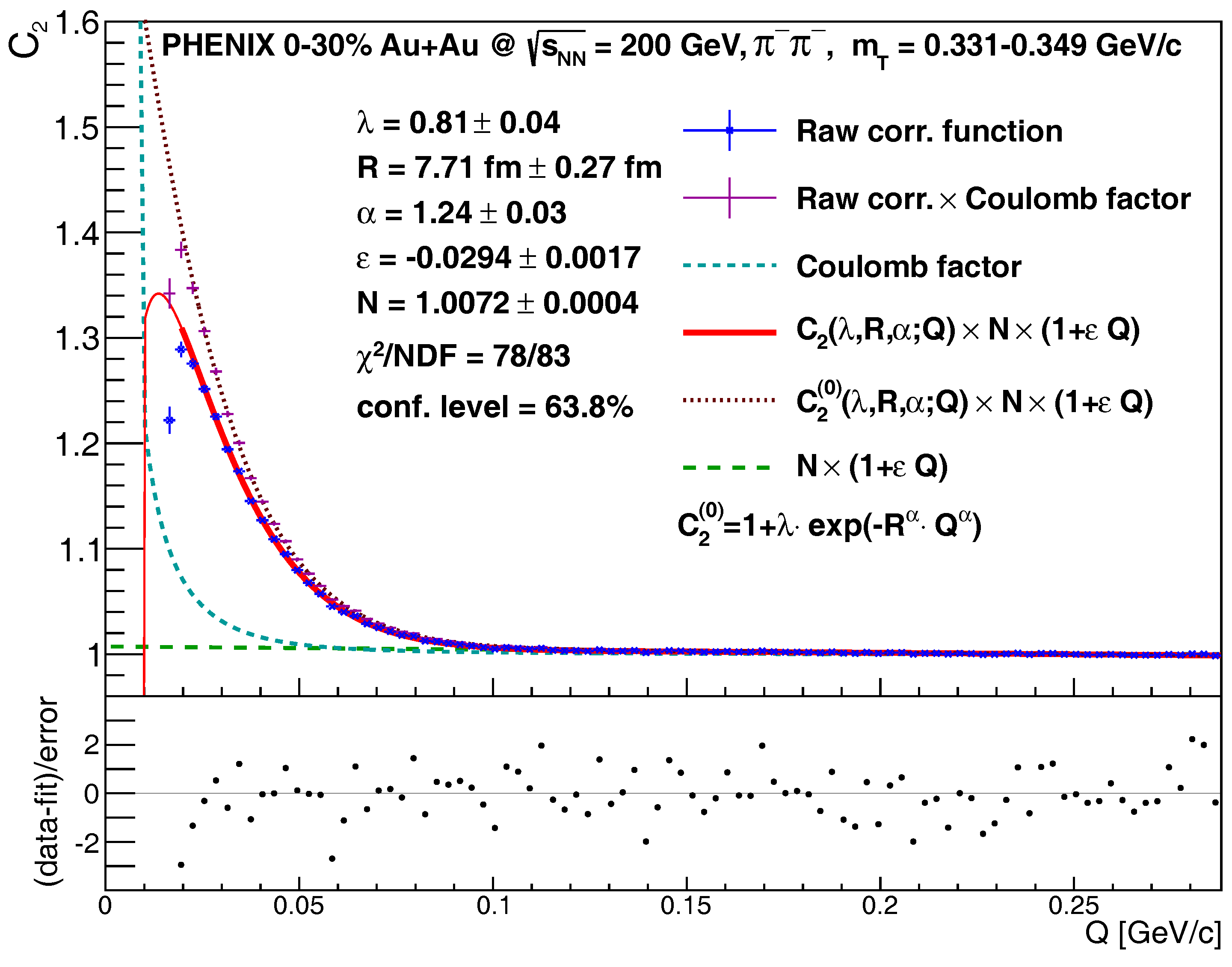
We analyzed 2.2 billion 0–30% centrality 200 GeV Au + Au collisions recorded by the PHENIX experiment in the 2010 running period1. We measured two-particle correlation functions of and pairs, in 31 bins ranging from 228 to 871 MeV, as detailed in Ref. [13]. The calculated correlation functions based on Lévy-shaped sources gave statistically acceptable descriptions of all measured correlation functions (all transverse momenta and both charges), see for example Figure 1. Note that besides the event selection and the track selection criteria discussed in Ref. [13], we applied two-track cuts as well, to remove merged tracks and “ghost” tracks, both of which appear due to the spatial two-track resolution of our tracking system. This removes the very small Q part of the correlation functions, as seen in Figure 1. A reminiscence of this is seen from the lowest Q point in Figure 1: this defines our fit range. The effect of the choice of the fit range and the two-track cuts was studied and incorporated into the systematic uncertainties. See more details about this topic also in Ref. [13]. The fact that the correlation functions were described by Lévy fits allows us to study and interpret the dependence of the fit parameters R, and , as they do represent the measured correlation functions.
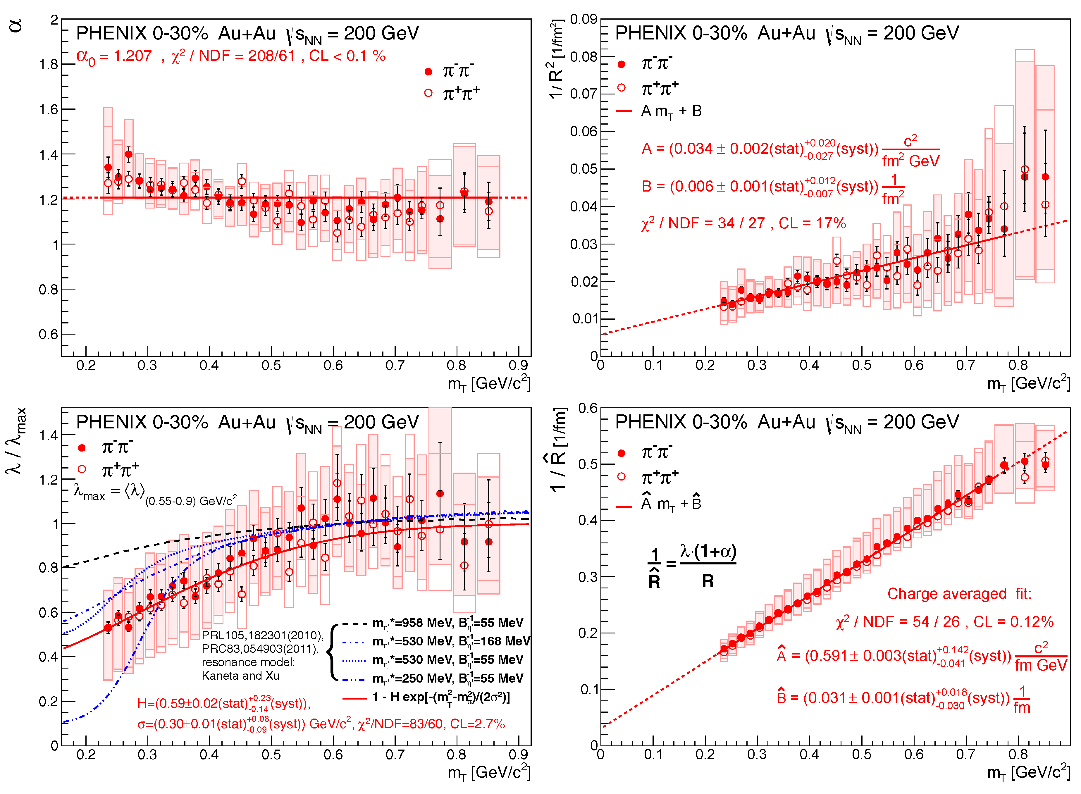
Let us turn to the resulting fit parameters and their dependence. Parameters , R and are shown in Figure 2, as a function of pair (corresponding to the given bin). The detailed description of the systematic uncertainties is given in Ref. [13], here we focus on the characteristics of the dependencies. In the top left panel of Figure 2, we observe that is constant within systematic uncertainties, with an average value of 1.207. This average value is far from the Gaussian assumption of as well as from the conjectured value at the critical point. We show as a function of on the top right panel of Figure 2. We observe, that the hydro prediction of still holds—even though in hydrodynamics, usually no power-law tails appear, due to the Boltzmann factor creating an exponential cut-off. This is intriguing point may be investigated in phenomenological models in the future. The correlation function intercept parameter is shown in the bottom left panel of Figure 2, after a normalization by
as detailed in Ref. [13]. The dependence of indicates a decrease at small . This may be explained by the increase of the resonance pion fraction at low . Such an increase is predicted to occur in case of an in-medium mass, as discussed above. It is interesting to observe that our data are not incompatible with predictions [28] based on a reduced mass, using the Kaneta-Xu model for ratios of long-lived resonances [29]. Finally, in the bottom right panel of Figure 2 we show the observation of a new scaling parameter
The inverse of this variable exhibits a clear linear scaling with , and it also has much decreased statistical uncertainties. Let us conclude by inviting the theory/phenomenology community to calculate the dependence of the above Lévy parameters, and compare their result to the measurements.
Acknowledgments
M. Cs. was supported by the New National Excellence program of the Hungarian Ministry of Human Capacities, the NKFIH grant FK-123842 and the János Bolyai Research Scholarship.
Conflicts of Interest
The author declares no conflict of interest.
References
- Adcox, K.; Adler, S.S.; Afanasiev, S.; Aidala, C.; Ajitanand, N.N.; Akiba, Y.; Al-Jamel, A.; Alexander, J.; Amirikas, R.; Aoki, K.; et al. Formation of dense partonic matter in relativistic nucleus nucleus collisions at RHIC: Experimental evaluation by the PHENIX collaboration. Nucl. Phys. A 2005, 757, 184–283. [Google Scholar] [CrossRef]
- Adams, J.; Aggarwal, M.M.; Ahammed, Z.; Amonett, J.; Anderson, B.D.; Arkhipkin, D.; Averichev, G.S.; Badyal, S.K.; Bai, Y.; Balewski, J.; et al. Experimental and theoretical challenges in the search for the quark gluon plasma: The STAR collaboration’s critical assessment of the evidence from RHIC collisions. Nucl. Phys. A 2005, 757, 102–183. [Google Scholar] [CrossRef]
- Arsene, I.; Bearden, I.G.; Beavis, D.; Besliu, C.; Budick, B.; Bøggild, H.; Chasman, C.; Christensen, C.H.; Christiansen, P.; Cibor, J.; et al. Quark gluon plasma and color glass condensate at RHIC? The Perspective from the BRAHMS experiment. Nucl. Phys. A 2005, 757, 1–27. [Google Scholar] [CrossRef]
- Back, B.B.; Baker, M.D.; Ballintijn, M.; Barton, D.S.; Becker, B.; Betts, R.R.; Bickley, A.A.; Bindel, R.; Budzanowski, A.; Busza, W.; et al. The PHOBOS perspective on discoveries at RHIC. Nucl. Phys. A 2005, 757, 28–101. [Google Scholar] [CrossRef]
- Hanbury Brown, R.; Twiss, R.Q. A Test of a new type of stellar interferometer on Sirius. Nature 1956, 178, 1046–1048. [Google Scholar] [CrossRef]
- Goldhaber, G.; Fowler, W.B.; Goldhaber, S.; Hoang, T.F. Pion-pion correlations in antiproton annihilation events. Phys. Rev. Lett. 1959, 3, 181–183. [Google Scholar] [CrossRef]
- Goldhaber, G.; Goldhaber, S.; Lee, W.Y.; Pais, A. Influence of Bose-Einstein statistics on the antiproton proton annihilation process. Phys. Rev. 1960, 120, 300–312. [Google Scholar] [CrossRef]
- Yano, F.B.; Koonin, S.E. Determining Pion Source Parameters in Relativistic Heavy Ion Collisions. Phys. Lett. B 1978, 78, 556–559. [Google Scholar] [CrossRef]
- Adler, S.S.; Afanasiev, S.; Aidala, C.; Ajitanand, N.N.; Akiba, Y.; Alexander, J.; Amirikas, R.; Aphecetche, L.; Aronson, S.H.; Averbeck, R.; et al. Bose-Einstein correlations of charged pion pairs in Au + Au collisions at s(NN)**(1/2) = 200 GeV. Phys. Rev. Lett. 2004, 93. [Google Scholar] [CrossRef] [PubMed]
- Afanasiev, S.; Aidala, C.; Ajitanand, N.N.; Akiba, Y.; Alexander, J.; Al-Jamel, A.; Aoki, K.; Aphecetche, L.; Armendariz, R.; Aronson, S.H.; et al. Kaon interferometric probes of space-time evolution in Au + Au collisions at s(NN)**(1/2) = 200 GeV. Phys. Rev. Lett. 2009, 103. [Google Scholar] [CrossRef] [PubMed]
- Makhlin, A.N.; Sinyukov, Y.M. The hydrodynamics of hadron matter under a pion interferometric microscope. Z. Phys. C 1988, 39, 69–73. [Google Scholar] [CrossRef]
- Csörgő, T.; Lörstad, B. Bose-Einstein Correlations for Three-Dimensionally Expanding, Cylindrically Symmetric, Finite Systems. Phys. Rev. C 1996, 54, 1390–1403. [Google Scholar] [CrossRef]
- Adare, A.; Aidala, C.; Ajitanand, N.N.; Akiba, Y.; Akimoto, R.; Alexander, J.; Alfred, M.; Al-Ta’ani, H.; Angerami, A.; Aoki, K.; et al. Lévy-stable two-pion Bose-Einstein correlations in GeV Au+Au collisions. arXiv, 2017; arXiv:1709.05649. [Google Scholar]
- Afanasiev, S.; Aidala, C.; Ajitanand, N.N.; Akiba, Y.; Alexander, J.; Al-Jamel, A.; Aoki, K.; Aphecetche, L.; Armendariz, R.; Aronson, S.H.; et al. Source breakup dynamics in Au + Au Collisions at s(NN)**(1/2) = 200 GeV via three-dimensional two-pion source imaging. Phys. Rev. Lett. 2008, 100. [Google Scholar] [CrossRef] [PubMed]
- Adler, S.S.; Afanasiev, S.; Aidala, C.; Ajitanand, N.N.; Akiba, Y.; Alexander, J.; Amirikas, R.; Aphecetche, L.; Aronson, S.H.; Averbeck, R.; et al. Evidence for a long-range component in the pion emission source in Au + Au collisions at s(NN)**(1/2) = 200 GeV. Phys. Rev. Lett. 2007, 98. [Google Scholar] [CrossRef] [PubMed]
- Metzler, R.; Barkai, E.; Klafter, J. Anomalous Diffusion and Relaxation Close to Thermal Equilibrium: A Fractional Fokker-Planck Equation Approach. Phys. Rev. Lett. 1999, 82, 3563–3567. [Google Scholar] [CrossRef]
- Csörgő, T.; Hegyi, S.; Zajc, W.A. Bose-Einstein correlations for Levy stable source distributions. Eur. Phys. J. C 2004, 36, 67–78. [Google Scholar] [CrossRef]
- Csanád, M.; Csörgő, T.; Nagy, M. Anomalous diffusion of pions at RHIC. Braz. J. Phys. 2007, 37, 1002–1013. [Google Scholar] [CrossRef]
- Csörgő, T. Correlation Probes of a QCD Critical Point. arXiv, 2008; arXiv:0903.0669. [Google Scholar]
- El-Showk, S.; Paulos, M.F.; Poland, D.; Rychkov, S.; Simmons-Duffin, D.; Vichi, A. Solving the 3D Ising Model with the Conformal Bootstrap II. c-Minimization and Precise Critical Exponents. J. Stat. Phys. 2014, 157, 869–914. [Google Scholar] [CrossRef]
- Rieger, H. Critical behavior of the three-dimensional random-field Ising model: Two-exponent scaling and discontinuous transition. Phys. Rev. B 1995, 52, 6659–6667. [Google Scholar] [CrossRef]
- Halasz, M.A.; Jackson, A.D.; Shrock, R.E.; Stephanov, M.A.; Verbaarschot, J.J.M. On the phase diagram of QCD. Phys. Rev. D 1998, 58. [Google Scholar] [CrossRef]
- Stephanov, M.A.; Rajagopal, K.; Shuryak, E.V. Signatures of the tricritical point in QCD. Phys. Rev. Lett. 1998, 81, 4816–4819. [Google Scholar] [CrossRef]
- Vance, S.E.; Csörgő, T.; Kharzeev, D. Partial U(A)(1) restoration from Bose-Einstein correlations. Phys. Rev. Lett. 1998, 81, 2205–2208. [Google Scholar] [CrossRef]
- Kapusta, J.I.; Kharzeev, D.; McLerran, L.D. The Return of the prodigal Goldstone boson. Phys. Rev. D 1996, 53, 5028–5033. [Google Scholar] [CrossRef]
- Novák, T.; Csörgő, T.; Eggers, H.C.; de Kock, M. Model independent analysis of nearly Lévy correlations. Acta Phys. Pol. Suppl. 2016, 9, 289. [Google Scholar] [CrossRef]
- Kincses, D. PHENIX results on Lévy analysis of Bose-Einstein correlation functions. Acta Phys. Pol. Suppl. 2017, 10, 627–632. [Google Scholar]
- Vértesi, R.; Csörgő, T.; Sziklai, J. Significant in-medium η’ mass reduction in GeV Au + Au collisions at the BNL Relativistic Heavy Ion Collider. Phys. Rev. C 2011, 83. [Google Scholar] [CrossRef]
- Kaneta, M.; Xu, N. Centrality dependence of chemical freeze-out in Au + Au collisions at RHIC (QM2004 proceedings). arXiv, 2004; arXiv:nucl-th/0405068. [Google Scholar]
| 1. |
Figure 1.
Example fit of pairs with between 0.331 and 0.349 GeV/c (corresponding to GeV/c), measured in the longitudinal co-moving frame. The fit shows the measured correlation function and the complete fit function, while a “Coulomb-corrected” fit function is also shown, with the data multiplied by .

Figure 2.
Fit parameters (top left), R (top right, shown as ), (bottom left, shown as ) and (bottom right, shown as ) versus average of the pair. Statistical and symmetric systematic uncertainties shown as bars and boxes, respectively.
Figure 2.
Fit parameters (top left), R (top right, shown as ), (bottom left, shown as ) and (bottom right, shown as ) versus average of the pair. Statistical and symmetric systematic uncertainties shown as bars and boxes, respectively.

© 2017 by the author. Licensee MDPI, Basel, Switzerland. This article is an open access article distributed under the terms and conditions of the Creative Commons Attribution (CC BY) license (http://creativecommons.org/licenses/by/4.0/).
Share and Cite
MDPI and ACS Style
Csanád, M. Lévy Femtoscopy with PHENIX at RHIC. Universe 2017, 3, 85. https://doi.org/10.3390/universe3040085
AMA Style
Csanád M. Lévy Femtoscopy with PHENIX at RHIC. Universe. 2017; 3(4):85. https://doi.org/10.3390/universe3040085
Chicago/Turabian StyleCsanád, Máté. 2017. "Lévy Femtoscopy with PHENIX at RHIC" Universe 3, no. 4: 85. https://doi.org/10.3390/universe3040085
APA StyleCsanád, M. (2017). Lévy Femtoscopy with PHENIX at RHIC. Universe, 3(4), 85. https://doi.org/10.3390/universe3040085
Note that from the first issue of 2016, this journal uses article numbers instead of page numbers. See further details here.