Universal Hyperbolic Geometry, Sydpoints and Finite Fields: A Projective and Algebraic Alternative

Abstract

Universal hyperbolic geometry gives a purely algebraic approach to the subject that connects naturally with Einstein’s special theory of relativity. In this paper, we give an overview of some aspects of this theory relating to triangle geometry and in particular the remarkable new analogues of midpoints called sydpoints. We also discuss how the generality allows us to consider hyperbolic geometry over general fields, in particular over finite fields.

1. Two Famous Questions and a Projective/Algebraic Look at Hyperbolic Geometry

While physicists have long pondered the question of the physical nature of the “continuum”, mathematicians have struggled to similarly understand the corresponding mathematical structure. In the last decade, we have seen the emergence of rational trigonometry [1,2] as a viable alternative to traditional geometry, built not over a continuum of “real numbers”, but rather algebraically over a general field, so also over the rational numbers, or over finite fields.

Universal hyperbolic geometry (UHG) extends this understanding to the projective setting, yielding a new and broader approach to the Cayley–Klein framework (see [3]) for the remarkable geometry discovered now almost two centuries ago by Bolyai, Gauss and Lobachevsky as in [4,5,6]. See also [7,8] for the classical and modern use of projective metrical structures in geometry. In this paper, we will give an outline of this new approach, which connects naturally to the relativistic geometry of Lorentz, Einstein and Minkowski and also allows us to consider hyperbolic geometries over general fields, including finite fields.

To avoid technicalities and make the subject accessible to a wider audience, including physicists, we aim to describe things both geometrically in a projective visual fashion, as well as algebraically in a linear algebraic setting.

2. The Polarity of a Conic Discovered by Apollonius

We augment the projective plane, which we may regard as a two-dimensional affine plane and a line at infinity, with a fixed conic. This conic is called the absolute in Cayley–Klein geometry. In this universal hyperbolic geometry (UHG), developed in [9,10,11,12], we take it to be a circle, typically in blue, and call it the null circle.

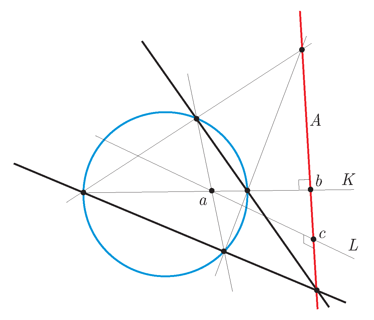
The polarity associated with a conic was investigated by Apollonius and gives a duality between points a and lines $A=a^{\perp }$ in the space, which we also write as $a=A^{\perp }.$ Given a point $a,$ consider any two lines through a, which meet the conic at two points each as in Figure 1. The other two diagonal points of this cyclic quadrilateral defines the dual line $A.$ Remarkably, this construction does not depend on the choice of lines through $a,$ as Apollonius realized.

Figure 1. The dual of a point a is a line $a=A^{\perp }$.

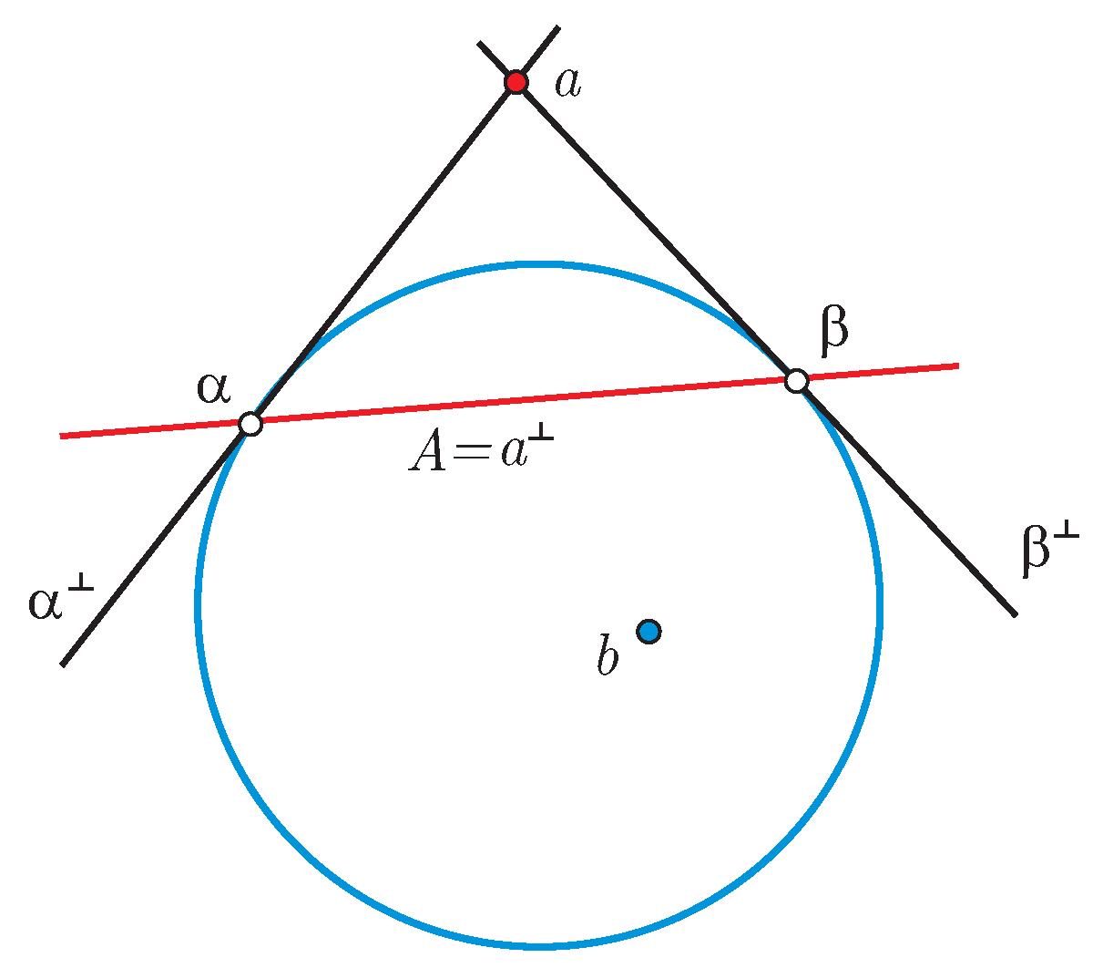
When a approaches the conic, the dual A approaches the tangent to the conic at that point. If b lies on $A=a^{\perp },$ then it turns out that a lies on $B=b^{\perp }.$

From this duality, we may define the perpendicularity, which lies at the core of hyperbolic geometry. Two points are perpendicular when one lies on the dual of the other, and similarly two lines are perpendicular when one passes through the dual of the other. We treat points and lines symmetrically!

Hyperbolic geometry is then the study of those aspects of projective geometry that are determined by the fixed conic, with isometries just those projective transformations, which fix the null circle. This turns out to be essentially the relativistic group $O\left(2,1\right),$ with coefficients in the base field, as we shall see. However, to describe the actual metrical structure, we move beyond the usual hyperbolic distance and angle found in the classical theory of Bolyai, Gauss and Lobachevsky; rather, we employ hyperbolic analogues of the quadrance and spread of rational trigonometry.

3. Null Points, Lines and Light Cones

Null points are perpendicular to themselves; these are the points lying on the original null circle, such as $\alpha$ and $\beta$ in Figure 2. Null lines are also perpendicular to themselves; these are just duals of null points or the tangents to the null circle, as shown in Figure 2. In classical hyperbolic geometry, only the interior of the circle is usually considered, and the absolute circle is considered to be “infinitely far away”. Here, we are interested in the entire projective plane, including also the null conic itself and its exterior, including actually points at infinity.

Figure 2. Null points and null lines on the null conic.

This corresponds to considering a $2+1$ relativistic space projectively: with the null conic corresponding to the light cone; points inside the null conic to time-like directions; and points outside the null conic to space-like directions. Like the physicist, we regard the entire space as of primary interest, not just the interior of our light cone, even if this is our initial orientation!

The usual geometry of special relativity in $2+1$ dimensions, in a vector space with inner product:

$$\left(x_1,y_1,z_1\right)·\left(x_2,y_2,z_2\right)=x_1{x}_2+y_1{y}_2-z_1{z}_2$$

(1)

when looked at projectively, gives us UHG, with the null cone $x^2+y^2-z^2=0$. The usual hyperboloid of two sheets $x^2+y^2-z^2=-1$, the top sheet of which classically corresponds to the hyperbolic plane, is a Riemannian sub-manifold of the Lorentzian three-dimensional space. This variant of Euclidean structure holds in the interior of the null conic, but outside, we are in a de Sitter-type space as represented by the hyperboloid of one sheet $x^2+y^2-z^2=1$. This kind of universal hyperbolic geometry is no longer homogeneous, as points outside the null conic behave differently from points inside the conic, and indeed over more general fields, the distinction between these two types of points is considerably more subtle.

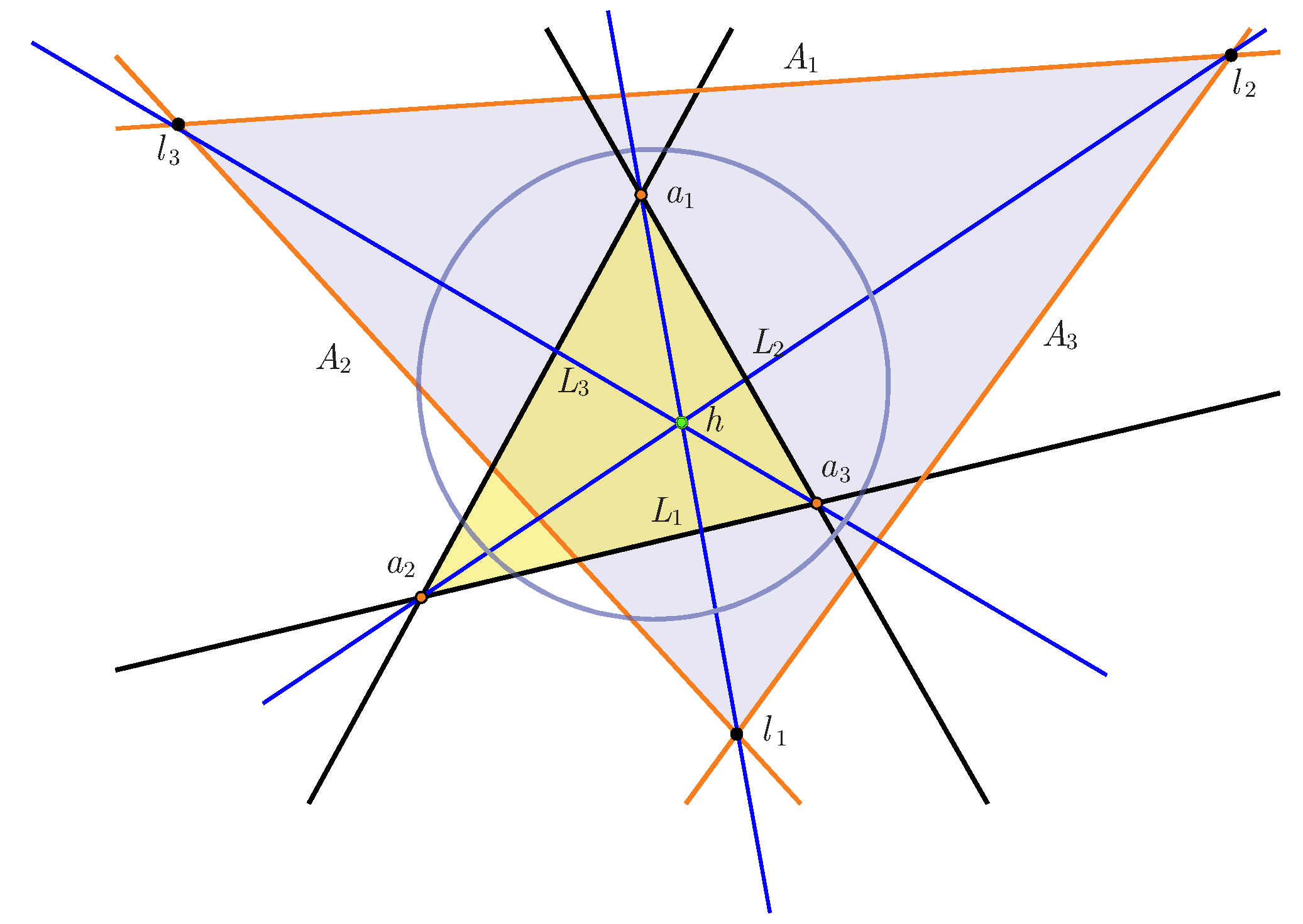
4. Triangle and Dual

To see, the importance and usefulness of considering both interior and exterior points, let us look at a triangle $\overline{a_1{a}_2{a}_3}$ with sides the lines $L_1,L_2,L_3,$ and its dual triangle $\overline{l_1{l}_2{l}_3},$ with sides $A_1,A_2$ and $A_3.$ These two triangles play now a symmetrical role: the duals of the points $a_1,a_2,a_3$ are the lines $A_1,A_2,A_3,$ while the duals of the points $l_1,l_2,l_3$ are the lines $L_1,L_2,L_3.$

The dual triangle plays a natural role in establishing the existence of an orthocenter of a general triangle, which is a valid theorem in this form of hyperbolic geometry, although it is not in classical hyperbolic geometry! In Figure 3, we see the three altitudes of the triangle $\overline{a_1{a}_2{a}_3}$ determined by lines from vertices to dual vertices, meeting at the orthocenter $h.$ The reason that this does not work in general in classical hyperbolic geometry is that the meeting of the three altitudes may well be outside the null conic even if all three points of the triangle are inside, and so it is invisible to the geometry of Bolyai, Gauss and Lobachevsky! Since this anecdotally was one of Einstein’s favourite geometry theorems, it is definitely worthwhile having it as part of the picture.

Figure 3. The dual triangle and the orthocenter h.

In fact, a similar discussion may be had for the circumcenter. This is all part of the rich and mostly new subject of hyperbolic triangle geometry; see for example [11,13,14], which recently has also been extended to include quadrilateral geometry in [15].

5. Quadrance May Be Defined Algebraically

In classical hyperbolic geometry, the metrical structure is introduced using differential geometry in the context of Riemannian metrics on smooth manifolds. In the more projective situation, as in [16], the notions of projective quadrance and projective spread can be introduced using the fundamental idea of a cross-ratio of four points on a line, as appreciated also by [17].

If four collinear points have projective coordinates $a,b,c$ and d, which can be either from the given field or possibly have the value infinity (∞), then their cross-ratio may be defined as:

$$\left(a,b:c,d\right)\equiv \frac{\left(c-a\right)\left(d-b\right)}{\left(c-b\right)\left(d-a\right)}.$$

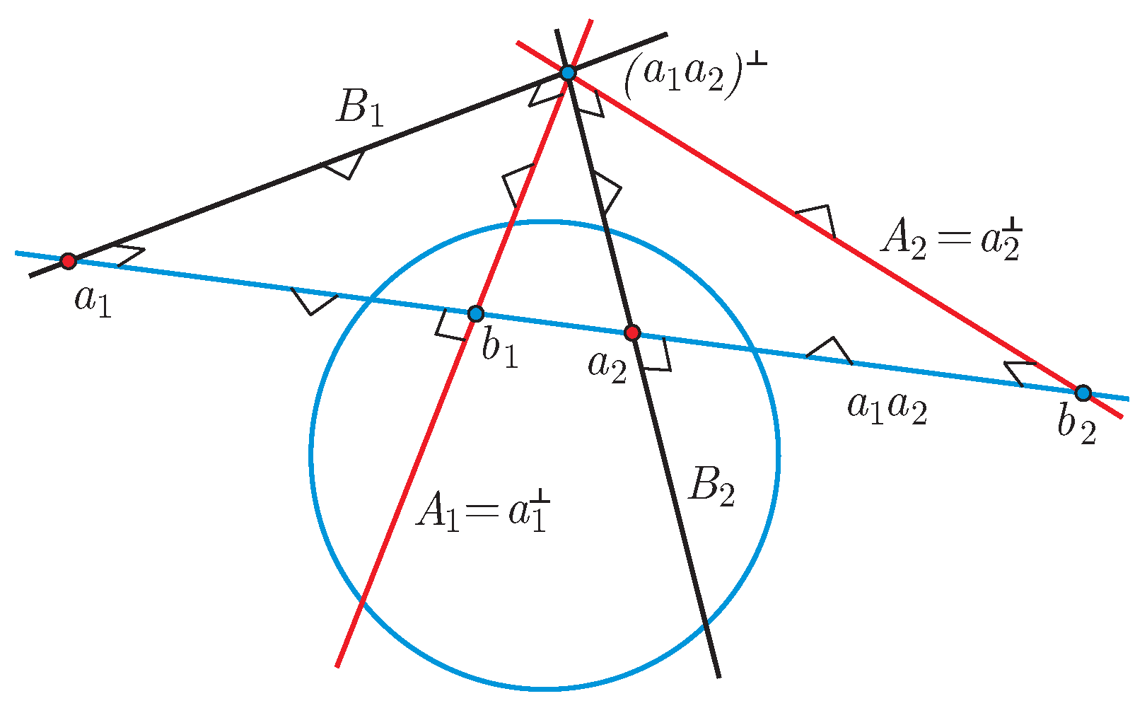
Now, given two points $a_1$ and $a_2$ in the hyperbolic plane, they have dual lines $A_1$ and $A_2,$ which meet the line $a_1{a}_2$ in the conjugate points:

$$b_1\equiv A_1\left(a_1{a}_2\right)\mathrm{and}{b}_2\equiv A_2\left(a_1{a}_2\right)$$

giving four collinear points $a_1,a_2,b_1$ and $b_2.$ Then, the (projective) quadrance between $a_1$ and $a_2$ is the cross-ratio:

$$q\left(a_1,a_2\right)\equiv \left(a_1,b_2:a_2,b_1\right).$$

In Figure 4, we see an example of $a_1$ exterior and $a_2$ interior, to emphasize the case that this metrical notion applies very generally to all non-null points.

Figure 4. Conjugate points make a cross-ratio.

Define the spread between lines dually, so that:

$$S\left(A_1,A_2\right)\equiv q\left(a_1,a_2\right).$$

In this way, the relation between the points and lines metrically is completely symmetric. There is a natural connection with the usual classical metrical notions in the Beltrami–Klein model (see [5]) when we restrict to interior points (inside the light cone or null conic) and lines that meet also at interior points; in these cases:

$$q\left(a_1,a_2\right)=-{sinh}^2\left(d\left(a_1,a_2\right)\right)\mathrm{and}S\left(L_1,L_2\right)={sin}^2\left(\theta \left(L_1,L_2\right)\right).$$

6. The Algebraic Approach

Due to the modern familiarity with linear algebra, it may be useful to reframe the projective setup above using homogeneous coordinates, where we follow: [9]. In a three-dimensional vector space of row vectors $\left(x,y,z\right)$, we may define a (hyperbolic) point $a\equiv \left[x:y:z\right]$ to be a one-dimensional subspace through a non-zero vector $\left(x,y,z\right).$ This corresponds to the planar point $\left[\frac{x}{z},\frac{y}{z}\right]$ if $z\ne 0.$

A (hyperbolic) line $L\equiv \left(l:m:n\right)$ may be defined to be a two-dimensional subspace with equation $lx+my-nz=0$. The incidence between these points and lines is that the point $a\equiv \left[x:y:z\right]$ lies on the line $L\equiv \left(l:m:n\right)$, or equivalently L passes through $a,$ precisely when:

$$lx+my-nz=0.$$

In matrix terms, this is the relation:

$$\left(\begin{array}{ccc}x& y& z\end{array}\right)\left(\begin{array}{ccc}1& 0& 0\\ 0& 1& 0\\ 0& 0& -1\end{array}\right)\left(\begin{array}{c}l\\ m\\ n\end{array}\right)=0.$$

The point $a\equiv \left[x:y:z\right]$ is then dual to the line $L\equiv \left(l:m:n\right)$ precisely when:

$$x:y:z=l:m:n.$$

In this case, we write $a^{\perp }=L$ or $L^{\perp }=a.$ This algebraic structure ensures that these definitions work over a general field.

The metrical structure comes about from the symmetric bilinear form (1) of Einstein, Lorentz and Minkowski of the ambient three-dimensional space. It may be used to define a relation between one-dimensional subspaces as follows: the quadrance between points $a_1\equiv \left[x_1:y_1:z_1\right]$ and $a_2\equiv \left[x_2:y_2:z_2\right]$ is:

$$q\left(a_1,a_2\right)\equiv 1-\frac{{\left(x_1{x}_2+y_1{y}_2-z_1{z}_2\right)}^2}{\left(x_1^2+y_1^2-z_1^2\right)\left(x_2^2+y_2^2-z_2^2\right)}.$$

Dually, the spread between lines $L_1\equiv \left(l_1:m_1:n_1\right)$ and $L_2\equiv \left(l_2:m_2:n_2\right)$ is:

$$S\left(L_1,L_2\right)\equiv 1-\frac{{\left(l_1{l}_2+m_1{m}_2-n_1{n}_2\right)}^2}{\left(l_1^2+m_1^2-n_1^2\right)\left(l_2^2+m_2^2-n_2^2\right)}.$$

For three points $a_1,a_2$ and $a_3,$ the three quadrances will be:

$$q_1=q\left(a_2,a_3\right)q_2=q\left(a_1,a_3\right)q_3=q\left(a_1,a_2\right)$$

and for three lines $L_1,L_2$ and $L_3,$ the three spreads will be:

$$S_1=S\left(L_2,L_3\right)S_2=S\left(L_1,L_3\right)S_3=S\left(L_1,L_2\right).$$

7. The Main Trigonometric Laws of UHG

Here are the main trigonometric laws in the subject, established first in [9]. We begin with essentially the one-dimensional situations:

Theorem 1 (Triple quad formula).

If $a_1,a_2$ and $a_3$ are collinear points, then:

$${\left(q_1+q_2+q_3\right)}^2=2\left(q_1^2+q_2^2+q_3^2\right)+4q_1{q}_2{q}_3.$$

Theorem 2 (Triple spread formula).

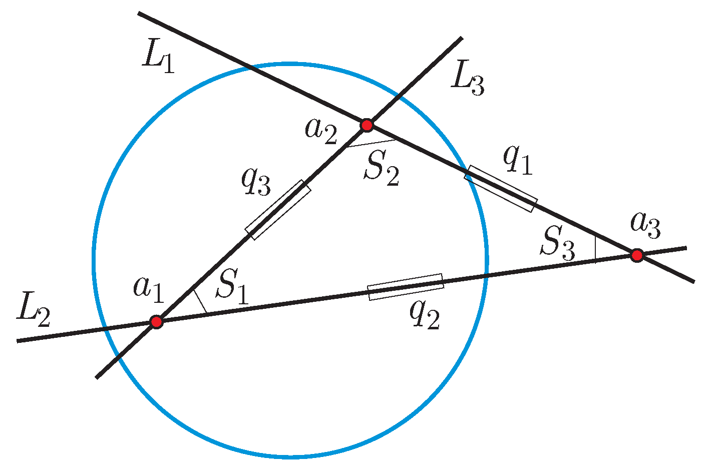
If $L_1,L_2$ and $L_3$ are concurrent lines, then:

$${\left(S_1+S_2+S_3\right)}^2=2\left(S_1^2+S_2^2+S_3^2\right)+4S_1{S}_2{S}_3.$$

Now, for the quadrances and spreads of a triangle $\overline{a_1{a}_2{a}_3}$ as in Figure 5:

Figure 5. Quadrance and spreads in a hyperbolic triangle.

Theorem 3 (Pythagoras).

If $L_1$ and $L_2$ are perpendicular lines, then:

$$q_3=q_1+q_2-q_1{q}_2.$$

Theorem 4 (Pythagoras dual).

If $a_1$ and $a_2$ are perpendicular points, then:

$$S_3=S_1+S_2-S_1{S}_2.$$

Theorem 5 (Spread law).

$$\frac{S_1}{q_1}=\frac{S_2}{q_2}=\frac{S_3}{q_3}.$$

Theorem 6 (Spread dual law).

$$\frac{q_1}{S_1}=\frac{q_2}{S_2}=\frac{q_3}{S_3}.$$

Theorem 7 (Cross law).

$${\left(q_1{q}_2{S}_3-\left(q_1+q_2+q_3\right)+2\right)}^2=4\left(1-q_1\right)\left(1-q_2\right)\left(1-q_3\right).$$

Theorem 8 (Cross dual law).

$${\left(S_1{S}_2{q}_3-\left(S_1+S_2+S_3\right)+2\right)}^2=4\left(1-S_1\right)\left(1-S_2\right)\left(1-S_3\right).$$

There are three symmetrical forms of Pythagoras’s theorem, the cross law and their duals, obtained by rotating indices. These various laws replace the transcendental hyperbolic Pythagoras’ theorem, the sine law and cosine law of both kinds. They work over a general field, both inside and outside the null circle, and actually even with more general bilinear forms. They are arguably more natural and convenient for physicists.

The quantity:

$$\mathcal{A}\equiv q_2{q}_3{S}_1=q_1{q}_3{S}_2=q_1{q}_2{S}_3$$

is the quadrea of the triangle $\overline{a_1{a}_2{a}_3}$ and is somewhat analogous to the hyperbolic area of the triangle, but it is decidedly of a different character. It is a big step to make the transition from transcendental to purely algebraic concepts here: computations can actually now be exhibited completely and clearly.

8. Circles, Midpoints and Circumcenters

A hyperbolic circle with centre a and quadrance k is the locus of points x, which satisfy $q\left(a,x\right)=k$. This is a conic, which includes what in the classical literature are called “equi-distant curves” in the case of an external centre.

A midpoint m of a side $\overline{a_1{a}_2}$ is a point lying on the line $a_1{a}_2$ that satisfies $q\left(a_1,m\right)=q\left(a_2,m\right)$. Midpoints exist precisely when $1-q\left(a_1,a_2\right)$ is a square in the field. There are in general two midpoints if they exist at all, and they are perpendicular. A midline is the dual of a midpoint, or equivalently a line through a midpoint perpendicular to the line joining the two original points; in other words, the hyperbolic version of a perpendicular bisector. The following is illustrated in Figure 6.

Figure 6. Circumcenters and circumlines of a triangle $\overline{a_1{a}_2{a}_3}$.

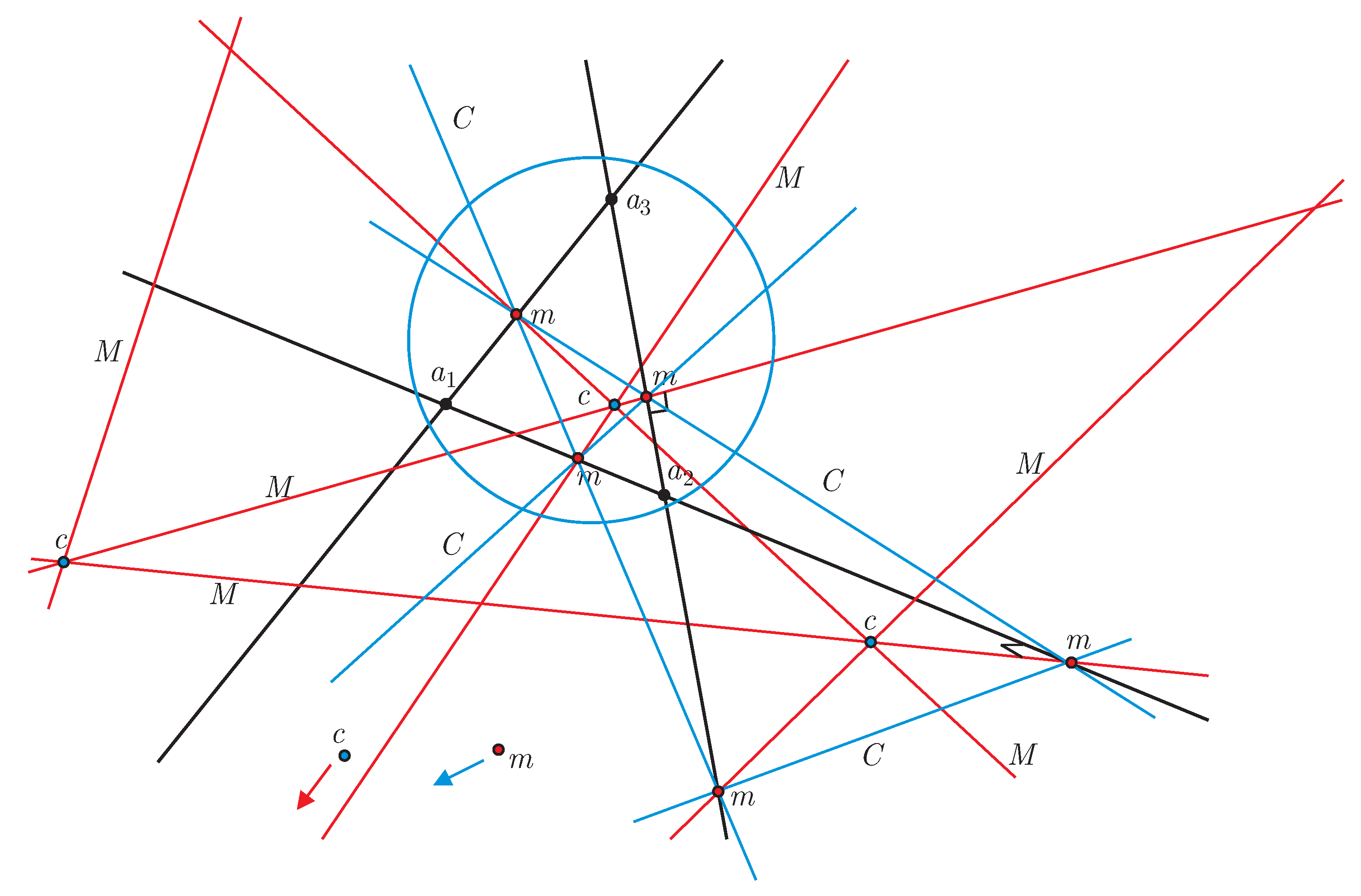
Theorem 9 (Circumcenters).

Assume that the six midpoints m of a triangle $\overline{a_1{a}_2{a}_3}$ exist. Then, they are collinear three at a time, lying on four distinct circumlines $C.$ The six midlines M of $\overline{a_1{a}_2{a}_3}$ are concurrent three at a time, meeting at four distinct circumcenters c that are dual to the circumlines C. The circumcenters are the centres of in general four hyperbolic circles that pass through the points of the triangle $\overline{a_1{a}_2{a}_3}$.

9. Sydpoints Augment Midpoints

While midpoints have been studied since the early days of the subject, an important related notion was only introduced very recently in [12]. A sydpoint of a side $\overline{a_1{a}_2}$ is a point s lying on $a_1{a}_2$ that satisfies $q(a_1,s)=-q(a_2,s).$ Sydpoints exist precisely when $q\left(a_1,a_2\right)-1$ is a square in the field. There are in general two sydpoints, if they exist at all, but they are not perpendicular.

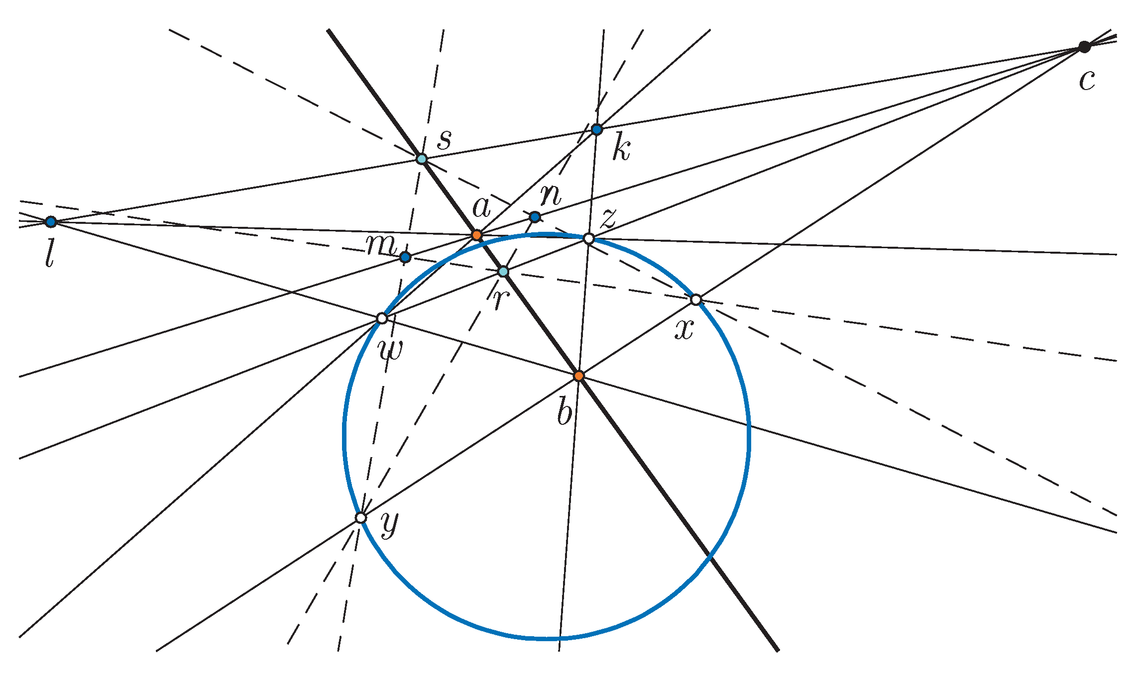
A construction of sydpoints r and s of $\overline{ab}$ may be deduced from Figure 7.

Figure 7. Construction of sydpoints.

First construct $c={\left(ab\right)}^{\perp }$, then the midpoints m and n of $\overline{ac}$ and then use the null points x and y lying on $bc$ as shown.

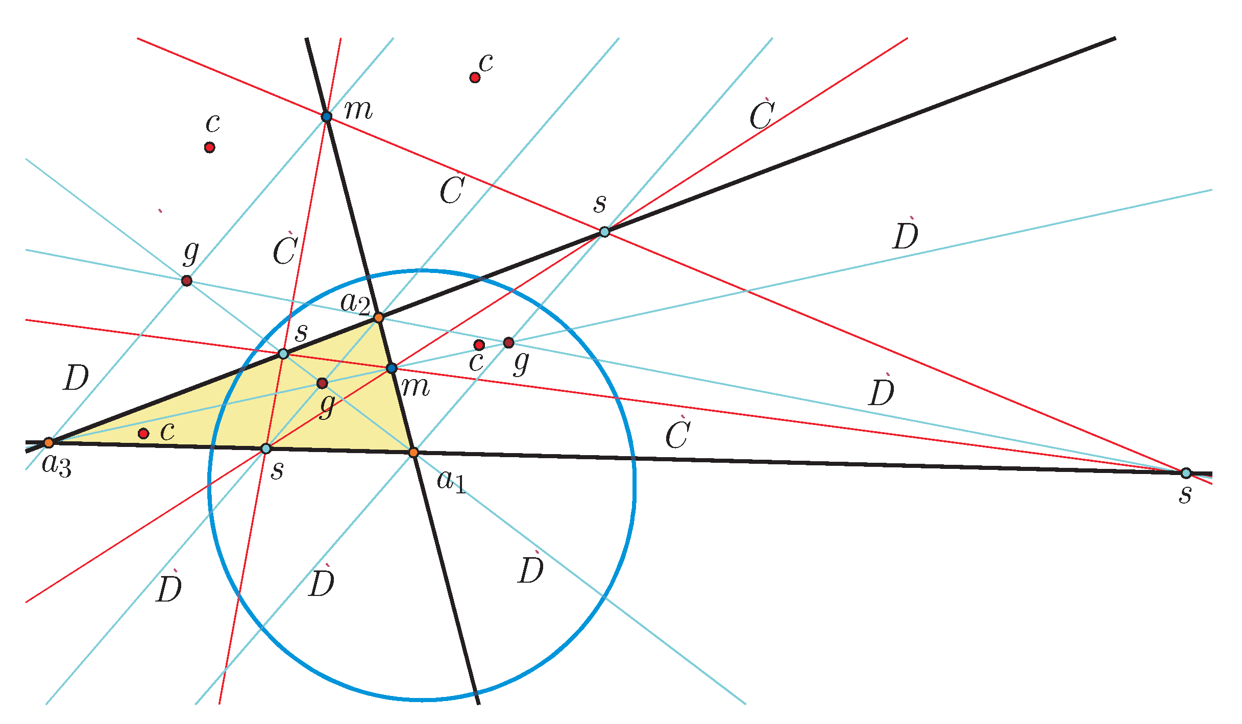
Sydpoints work with midpoints to extend triangle geometry to triangles with vertices both inside and outside the null conic. In Figure 8, we see centroids g and circumlines C of such a triangle. For the remarkable connection of the circumcenters c to circles through the three points, see [12].

Figure 8. Centroids and circumlines of a triangle.

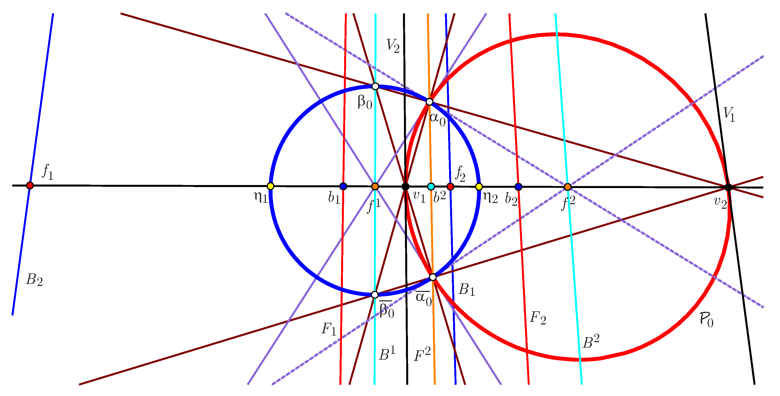
10. Sydpoints and the Parabola

In [18,19], we defined the hyperbolic parabola ${\mathcal{P}}_0$ to be the locus of a point $p_0$ (actually a conic) satisfying:

$$q(p_0,f_1)+q(p_0,f_2)=1$$

for fixed points $f_1,f_2$ called the foci. Equivalently:

$$q\left(p_0,f_1\right)=q\left(p_0,F_2\right)\mathrm{or}q\left(p_0,f_2\right)=q\left(p_0,F_1\right),$$

where $F_1\equiv f_1^{\perp },$ $F_2\equiv f_2^{\perp }$ are the directrices. Note that the quadrance between a point and a line is defined in terms of the perpendicular transversal. Such a parabola is shown in red in Figure 9.

Figure 9. A parabola with foci $f_1$ and $f_2$.

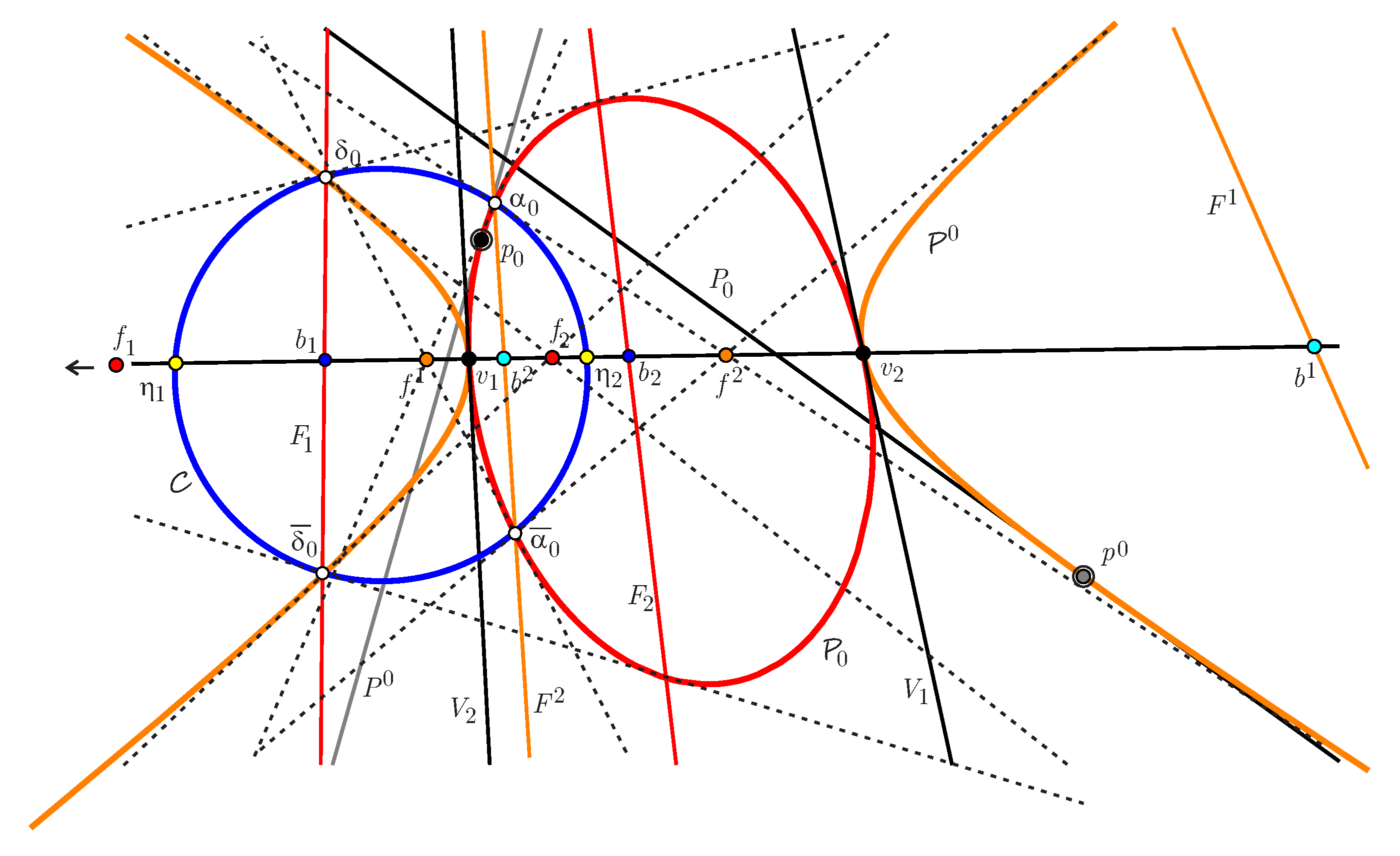
In general, if we take duals of the tangents of a conic, we get a dual conic. It turns out that the dual of a parabola $P_0$ is another parabola: the twin parabola ${\mathcal{P}}^0$ whose foci $f^1$, $f^2$ are the sydpoints of the original foci pair $f_1,f_2,$ shown in orange in Figure 10. Therefore, sydpoints appear prominently in the geometry of the parabola!

Figure 10. The twin parabola with foci $f^1$ and $f^2$.

11. UHG over Finite Fields

Can midpoints and sydpoints exist together? The conditions that $1-q\left(a,b\right)$ is a square and $q\left(a,b\right)-1$ is a square are not simultaneously satisfied over our usual number system, or over a field $F_p$ where $p\equiv 3$ mod $4.$ However, in the case of $F_p$ where $p\equiv 1$ mod $4,$ then $-1$ is a square, so both midpoints and sydpoints can exist together. This is an entirely new aspect of hyperbolic geometry that is invisible to us usually. However, how can we visualize UHG over a finite field?

Fortunately, a new and powerful program being developed by Michael Reynolds at University of New South Wales (UNSW) Sydney accomplishes exactly this. This program will hopefully be available for public use in the near future.

In fact, hyperbolic geometry over finite fields has been considered previously; see [20,21]. With UHG, we get a novel approach that unifies all these geometries over arbitrary fields, so freeing us from the reliance on a particular ideology with respect to the “continuum”.