Hot Accretion Flow in Two-Dimensional Spherical Coordinates: Considering Pressure Anisotropy and Magnetic Field

1
Key Laboratory for Research in Galaxies and Cosmology, Shanghai Astronomical Observatory, Chinese Academy of Sciences, 80 Nandan Road, Shanghai 200030, China
2
School of Physical Science and Technology, Shanghai Tech University, 393 Middle Huaxia Road, Pudong, Shanghai 201210, China
3
University of Chinese Academy of Sciences, 19A Yuquan Road, Beijing 100049, China
*
Author to whom correspondence should be addressed.
Universe 2019, 5(9), 197; https://doi.org/10.3390/universe5090197
Submission received: 24 June 2019
/
Revised: 9 September 2019
/
Accepted: 10 September 2019
/
Published: 12 September 2019
(This article belongs to the Special Issue Black Hole Physics and Astrophysics)
Abstract
:For systems with extremely low accretion rate, such as Galactic Center Sgr A* and M87 galaxy, the ion collisional mean free path can be considerably larger than its Larmor radius. In this case, the gas pressure is anisotropic to magnetic field lines. In this paper, we pay attention to how the properties of outflow change with the strength of anisotropic pressure and the magnetic field. We use an anisotropic viscosity to model the anisotropic pressure. We solve the two-dimensional magnetohydrodynamic (MHD) equations in spherical coordinates and assume that the accretion flow is radially self-similar. We find that the work done by anisotropic pressure can heat the accretion flow. The gas temperature is heightened when anisotropic stress is included. The outflow velocity increases with the enhancement of strength of the anisotropic force. The Bernoulli parameter does not change much when anisotropic pressure is involved. However, we find that the energy flux of outflow can be increased by a factor of 20 in the presence of anisotropic stress. We find strong wind (the mass outflow is about 70% of the mass inflow rate) is formed when a relatively strong magnetic field is present. Outflows from an active galactic nucleus can interact with gas in its host galaxies. Our result predicts that outflow feedback effects can be enhanced significantly when anisotropic pressure and a relatively powerful magnetic field is considered.
1. Introduction
Black hole accretion models can be divided into hot and cold types based on its temperature. Both models are in a prevalent trend. For example, outflow/jet generated from a cold thin disk has been studied by both analytical (e.g., [1,2,3]) and simulation works (e.g., [4,5,6]). Hot accretion flows also are promising topics since the pioneering works of [7,8,9]. More recently, numerous numerical simulations have been performed to study hot accretion flows (e.g., [10,11,12,13,14,15,16,17,18,19,20,21,22,23,24,25,26,27,28]). Hot accretion flow can be applied to both the low-luminosity active galactic nuclei (LLAGNs) (e.g., [29,30,31]) and hard and quiescent states of black hole X-ray binaries (e.g., [32,33,34,35,36,37,38,39,40]).
The observations of LLAGNs (e.g., [41,42,43,44,45,46]) and the hard state of black hole X-ray binaries ([47]) show that outflow can be launched from hot accretion flow. The launching mechanisms and properties of outflow have been studied by numerical simulations(e.g., [24,26,27,48,49,50,51]) and analytical works ([52,53,54,55,56,57,58]). Outflow can push away gas which surrounds the black hole at sub-parsec and parsec scales, and can finally affect the black hole accretion rate and the star formation rate of galaxies (e.g., [59,60,61,62,63,64,65,66]).
In hot accretion flow of extremely low-luminosity AGNs, such as Sgr A and M 87, the Coulomb mean free paths of ions and electrons are more significant than the length-scale of the system (, where G, M, and c are gravitational constant, black hole mass, and speed of light, respectively) ([67,68,69,70]). In extremely low-accretion-rate system (like the accretion flow in our galactic center), at first glance, the pressure is wholly anisotropic. However, particle-in-cell simulations show that wave-particle interactions can increase the effective collisional rate of particles (e.g., [71,72,73,74]). Therefore, the accretion flow is just weakly collisional. The pressure is not wholly anisotropic. In plasmas physics, plasmas are fundamentally nonlinear. One of the most straightforward nonlinear effects is trapping of particles in large-amplitude waves, in which the wave potential exceeds the particle kinetic energy. Trapping is most significant for resonant particles, which are moving at the wave phase speed. The trapped particles bounce back and forth between the potential walls and oscillate periodically. Nonlinear interaction can lead to stable states consisting of large-amplitude waves and related particle distributions of trapped and free populations. It is difficult to find these states. No general mathematic algorithms exist in nonlinear theory, and often perturbation expansions are used, leading to what is called weak plasma turbulence theory or perturbation theory. The starting point is the coupled system of Maxwell’s and Vlasov’s equations. Likewise, in our cases, we better treat non-ideal effects anisotropic as perturbation relative to the ideal fluid. It is, however, an open question exactly how well this approach compares to full kinetic theory calculations. There are some other works studying the extremely low-accretion-rate accretion flow by adding an anisotropic pressure to the ideal gas (e.g., [69,70]).
The electron collisional mean free path can be much larger than its Larmor radius when the accretion flows are weakly collisional. In this case, thermal conduction is anisotropic and along magnetic field lines ([75,76,77]). The conduction can influence the dynamics of the accretion flow significantly ([68,78]). For example, conduction can transport energy from the inner to the outer regions. The gas in the outer region can have higher specific energy, which helps produce outflow in the outer region ([79]).
The ion collisional mean free path can also be larger than its Larmor radius in a quite low-accretion-rate hot accretion flow. Therefore, the pressure perpendicular to the magnetic field line is different from that parallel to the magnetic field line ([69,80,81]). Reference [82] performed numerical simulations and studied the effects of anisotropic pressure on the dynamics of the hot accretion flow. In their work, they assume that magnetic pressure is at least four orders of magnitude smaller than gas pressure. They find that gas can be accreted to the central black hole due to angular momentum transfer by anisotropic pressure. Also, they find that extremely weak outflow can be produced. Observations to some accretion system indicate that the viscous coefficient (see [83] and references in that paper). Because , with B and p are magnetic field and gas pressure respectively, therefore, magnetic pressure is about 0.1 times gas pressure. We define the ratio of gas to magnetic pressure as . The effects of anisotropic pressure on accretion flow have not been studied when magnetic pressure is not significantly smaller than gas pressure () ([82]). In [82], the authors only studied the accretion flow with an extremely weak magnetic field. In their work, the magnetic pressure is at least four orders of magnitude smaller than the gas pressure. However, in reality, in hot accretion flows, magnetic pressure is just smaller as a factor of 10 (e.g., [83]). Thus, it is necessary to study the hot accretion flow with anisotropic pressure in relatively stronger magnetic fields. In the present work, we study the hot accretion flow with anisotropic pressure in a much stronger magnetic field ().
Reference [84] studied hot accretion flow with anisotropic pressure in one-dimensional cylindrical coordinates, which is too simplified. We study the more complicated case: we solve the two-dimensional magnetohydrodynamic (MHD) equations in two-dimensional spherical coordinates considering the different magnitude of anisotropic pressure and magnetic field. Two-dimensional solutions have significant advantages compared to one-dimensional solutions. For example, in a one-dimensional solution, outflows are assumed to be present. However, the detailed structures of outflow are unknown. In two-dimensional solutions, we have the detailed structure of outflows (e.g., the spatial distribution of outflow, velocity, temperature, density as the functions of spatial locations). The detailed structures of outflows (e.g., the opening angle) are essential parameters in active galactic nuclei studies ([64]). Therefore, it is quite important to obtain the two-dimensional solutions of hot accretion flows with anisotropic pressure. In the radial direction, we assume that the accretion flow is self-similar. The most fundamental paper on self-similar outflows is [1]. They illustrated hydromagnetic flows from accretion disks and the production of radio jets. We pay attention to how the outflow properties are affected by anisotropic pressure and the magnetic field.
2. Basic MHD Equations
The basic MHD equations describing accretion flows read:
Here, denote the density, is the velocity, p is the gas pressure. We use the non-relativistic Newtonian potential (). e is gas internal energy. We adopt an ideal gas equation of state , with being adiabatic index.
Numerical simulations show that the magnetic field can be divided into a large-scale ordered component and a small-scale turbulent component (e.g., [85,86,87]). In Equations (2), (4) and (5), represents the large-scale component of the magnetic field. In Equation (2), is the electric current density.
In Equation (2), represents angular momentum transfer by the turbulent magnetic field. We assume only has azimuthal component, see [10,58,88].
Here, , with and are sound speed and Keplerian angular velocity, respectively.
In the energy Equation (3), is the heating due to viscosity and magnetic dissipation. The heating rate can be decomposed into two terms,
with
and
The anisotropic pressure can be modeled by an anisotropic viscosity ([69,89,90]),
where is a unit vector in the direction of magnetic field, and is the unit tensor. The anisotropic viscosity . In the energy Equation (3), the last term is the heating due to the work done by anisotropic pressure. Here is the magnetic diffusivity.
Previous works (e.g., [86,87,91]) find in their simulations that in the main body region of the accretion flow, the magnetic field is mainly toroidal. A poloidal component of the magnetic field can also be present. The anisotropic pressure tensor is related to the magnetic field geometry. If the poloidal magnetic field is included, the anisotropic pressure term can be very complicated. We find it is hard to solve the equations analytically in this case. Therefore, in this paper, we mainly study the dominant toroidal component of the magnetic field as a first step due to numerical simplicity. We may use numerical simulations to study this issue again by including a poloidal magnetic field in the future. We expect that with the presence of a poloidal magnetic field, the jet can be formed, and the power of wind can be much larger.
We seek for the steady state, axisymmetric solutions of Equations (1)–(5) in spherical coordinates (r, , ). The tensor then has the form below,
and
We can get the continuity equation,
In this paper, the magnetic field only has a toroidal component.
The equation of energy is expressed as,
The induction equation can be presented as,
2.1. Self-Similar Solutions
As with previous works (e.g., [58,88,92,93,94]), we seek the radially self-similar solutions in the following forms:
where is the Keplerian velocity at , is density at , is the power index. We note that the self-similar approach cannot be applied to the region in the vicinity of the black hole.
Both and are proportional to , where . The viscous coefficients (, ) and magnetic diffusivity () also need to satisfy the self-similar assumption, they have the form,
The radial profiles of , and satisfy the radial self-similar condition. For example, in the energy Equation (19), the terms in both left- and right- hand sides are proportional to .
2.2. System of Differential Equations
2.3. Boundary Conditions
We solve the six differential Equations (28)–(33) to get the functions for six variables: and . We assume the accretion flow is evenly symmetric about the equatorial plane, then , and . Thus, we can get the boundary conditions.
At the equatorial plane, we have by symmetry,
We adopt . Putting these assumptions into Equations (28)–(33), we can get the boundary conditions, which has the form
We define a coefficient which describes the ratio of the gas pressure to the magnetic field.
We denote the coefficient at the equatorial plane as , and we set its value manually.
3. Results
We use the second-order Runge–Kutta method to solve Equations (28)–(33) numerically. The resolution is for all the cases. We integrate these equations from the equatorial plane () towards the rotational axis ().We find that at a certain angle, there is a numerical error: a singularity exists near the axis. Therefore, we stopped our integration at . We have done tests and find that the value of does not change with resolution. Previous two-dimensional self-similar solutions (e.g., [88,94]) also found an error when integrating. In these two works, the authors have also not obtained the solution from to 0. We think the reason for the numerical error should be that the self-similar assumption cannot be applied to the region close to the rotational axis. Indeed, in the black hole accretion field, some other works are using self-similar approach, the solution over the whole space is obtained (e.g., [92]). Whether we can achieve a whole space solution may depend on the physics studied and the assumptions made. We think the solution in the region of are still physical. There are two reasons. First, the solutions satisfy the equation and boundary conditions at . Second, the quantities derived at are physical. For the low-accretion-rate hot accretion flow, radiation can be neglected. In this case, from the hydrodynamical equations, we can see that the normalization unit of density () in the left and right-hand sides of the equations can be deleted. In other words, for the non-radiative accretion flows, the gas density normalization unit can be any value. The other properties of the accretion flow (e.g., temperature, velocity) cannot be changed with the change of normalization. The magnetic energy is scaled by the gas pressure. The gas pressure is proportional to density multiply temperature. Therefore, the normalization unit of magnetic energy can be any value. However, the ratio of magnetic pressure to gas pressure is fixed.
For the extremely low-accretion-rate accretion flow, the radiative cooling is very weak, almost all the viscous heating energy is stored in gas and advected to the central black hole ([40]). Therefore, in this paper, we assume that the advection parameter . As introduced above, observations ([83]) show that the viscosity coefficient is . In this paper, we set the viscous coefficient . In [69], the authors did stability analysis to the accretion flow with anisotropic pressure. They found that for linear perturbations, the flow is stable if . Therefore, in our paper, the maximum value of is set to be 0.4, which is slightly smaller than .The radial infall velocity is for hot accretion flow. If the outflow is absent, the mass accretion rate will be a constant with radius, correspondingly, the density profile is . Numerical simulations of hot accretion flow show that the radial profile of density can be described as a power-law function of r as is proportional to , with ([10,24]). In this paper, we set the radial power-law index of density to be . We have done several tests and find that the results do not change much if the value of n slightly changes. We set the resistivity coefficient .
3.1. Model with Weak Magnetic Field
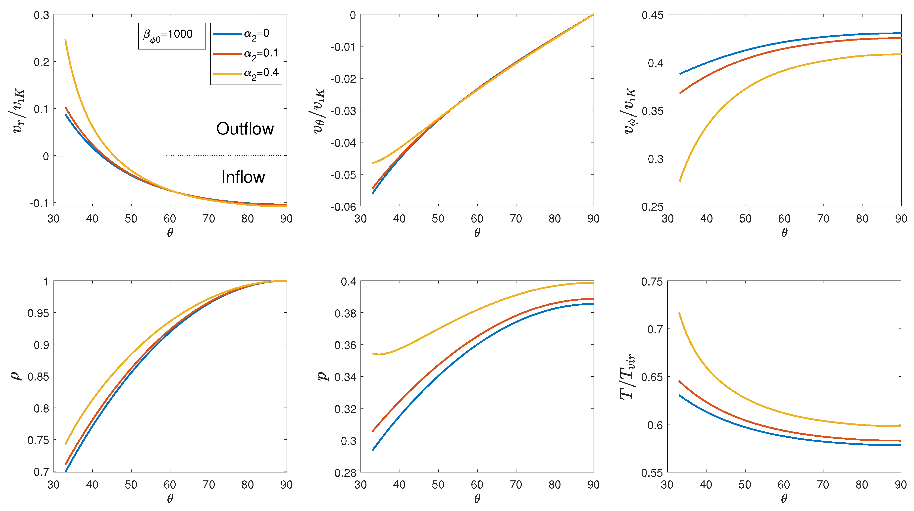
We first study the models with a weak magnetic field. We set the ratio of gas pressure to magnetic pressure , which means the gas pressure is 1000 times larger than the magnetic pressure in the midplane. Figure 1 plots angular profiles of velocities (), density (), pressure (p), and temperature (). The blue, red, and yellow lines correspond to , and , respectively. is the virial temperature, which is defined by,
where are the masses of proton and electron, k is Boltzmann constant. In this figure, we also show how the properties of accretion flow change with the strength of anisotropic pressure (denoted by , see Equation (10)). The mass density and pressure p decrease as decreases. Around the equator, it is the inflow region. changes its sign at a certain angle, denoted as . When , it is outflow region. is between –. From the last panel in Figure 1, we see that with the increase of the strength of anisotropic pressure (), the gas temperature increases. Correspondingly, the gas pressure rises with the increase of (see the bottom-middle panel). The accretion flow scale height ; therefore, the accretion flow in the model with has highest scale height. Correspondingly, in model with , the density decreases much slower towards the rotational axis (see bottom-left panel). From the top-left panel, we see that with the increase of , the outflow region widens.Also, the radial velocity of outflow increases. The reason is that for hot accretion flow, gas pressure gradient force is mainly responsible for driving outflow ([24]). When the anisotropic pressure increases, the gas pressure gradient increases. Therefore, the wind/outflow turns stronger. With the increase of gas temperature, outflows are more easily to be driven. The gas rotational velocity decreases with an increase of (see top-right panel). The reason is as follows. In the radial direction, the gravity is balanced by the gas pressure gradient and centrifugal forces. The gas pressure gradient force (or gas temperature) increases with . In order to keep the force balance, the centrifugal force (or rotational velocity) decreases with the increase of .
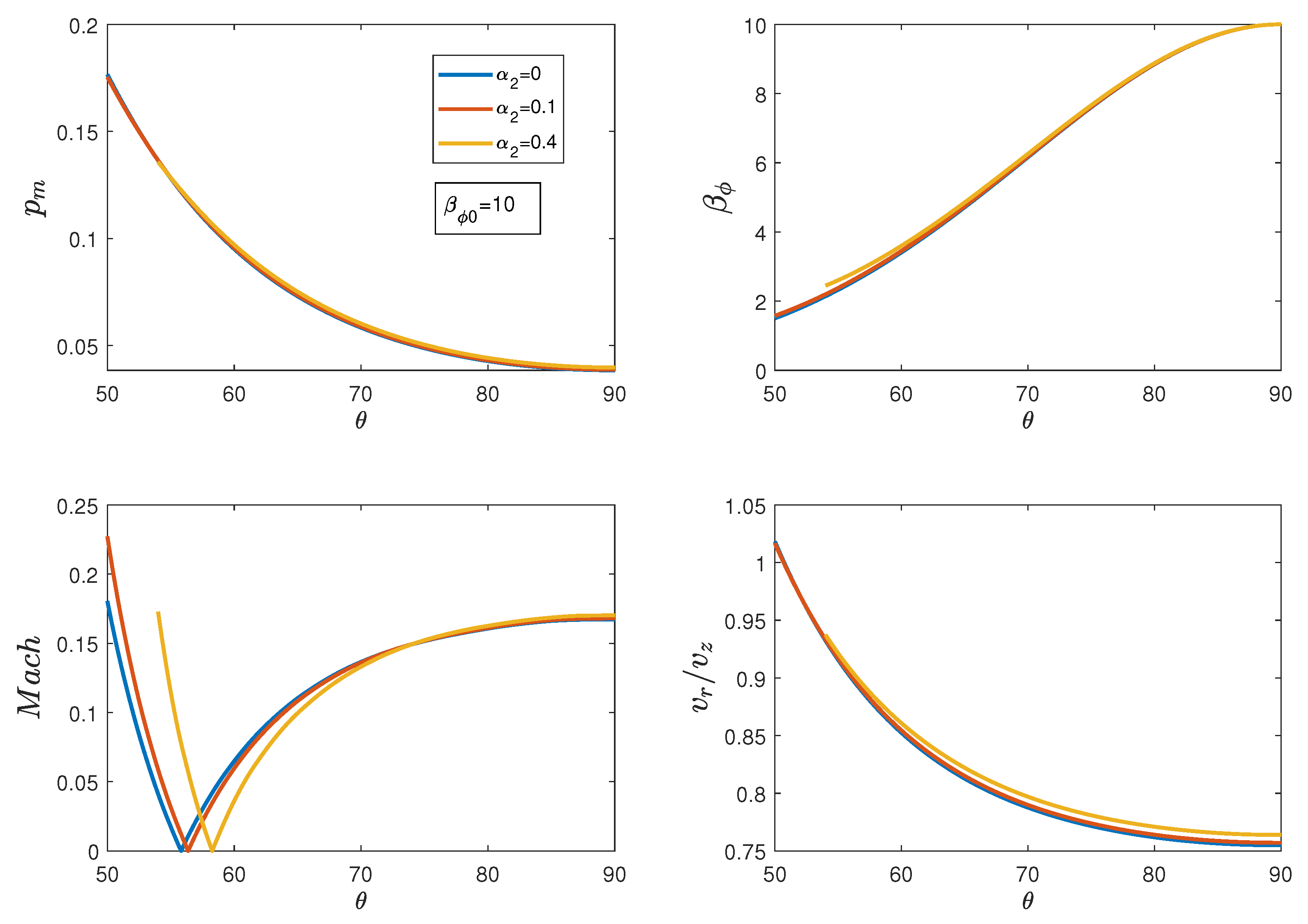
Figure 2 plots the magnetic pressure (), the ratio of gas pressure to magnetic pressure (), Mach number (), and change with . is the fast magnetosonic velocity, which is defined by:
where is the Alfvén velocity. In our case, . can be used to judge whether the flow passes the fast magnetosonic point or not. The blue, red, and yellow lines correspond to , and . The first panel in Figure 2 shows the magnetic pressure changes with . The strength of the magnetic pressure increases when decreases. However, it seems that the anisotropic pressure has no effect on the magnetic pressure. Please note that the values of are significantly larger compared to other variables. The magnetic pressure . Therefore, the change of the magnetic pressure is not apparent. The top-right panel in Figure 2 shows change with . The ratio of the gas pressure to the magnetic field decreases when decreases since the magnetic field turn stronger. The Mach number (see the bottom-left panel) increases when increases (). It has a minimum point when between 40–50 because changes its sign here. The Mach number is below 1. Therefore, the flow is subsonic. Because we assume that the accretion flow is radially self-similar, then the Mach number at any angle is a constant of the radius. The last panel of this figure shows that the flow does not pass the fast magnetosonic point in the weak magnetic model.
The work done by anisotropic pressure (the second term on the right-hand side of Equation (3)) heats the accretion flow.
Bernoulli parameter is usually used to judge whether outflow can escape from the black hole gravitational potential to infinity. In the magnetized accretion flow with only one toroidal magnetic field, the Bernoulli parameter is defined as,
Here, is enthalpy. Figure 3 plots the Bernoulli parameter in a unit of square Keplerian velocity. The Bernoulli parameter is positive as found by previous works (e.g., [9]). Because the magnetic field is quite weak, the magnetic term is quite small. The enthalpy term dominates other terms. The enthalpy is proportional to temperature. From Figure 1, we can see, with the increase of , the temperature increases. Therefore, the enthalpy increases with . Bernoulli parameter increases with .
The central black hole in a galaxy is believed to evolve with its host galaxy together. AGNs feedback plays a vital role in the evolution of galaxies. Outflow from black hole accretion flow can interact with the interstellar medium surrounding the AGN significantly. Outflow power is a crucial parameter in the AGN feedback study. Now, we study how the outflow power changes with . The power of outflow includes three components. They are kinetic, thermal powers, and Poynting flux. They are calculated as follows,
is the radial component of Poynting flux. If only is present, it is defined as,
Figure 4 shows how the outflow power changes with . Because the magnetic field is weak, the Poynting flux is quite small. The thermal energy carried by outflow dominates over other terms. With the increase of , gas temperature increases (see Figure 1). Correspondingly, the thermal energy flux carried by outflow increases. When , the total outflow power is 3–4 times larger than that when .
Now we calculate the ratio of mass inflow to outflow rates, and are defined as,
We find out that when the gas pressure is 1000 times larger than the magnetic pressure and the anisotropic pressure exists, the mass outflow rate is about 26%. In [82], their mass outflow rate is 10 to 15% of the mass inflow rate. Their wind is extremely weak due to their weak magnetic field ().
3.2. Model with Stronger Magnetic Fields
In black hole accretion flow, in the main body of the flow, it is always found that magnetic pressure is smaller than gas pressure by a factor of 10 (e.g., [14]). Therefore, in this section, we study relatively stronger magnetic field models with . Figure 5 plots angular profiles of velocities (), density (), pressure (p), and temperature (). The blue, red, yellow lines correspond to parameters , respectively. In this model, we set the gas pressure is ten times larger than the magnetic pressure at the midplane. Same as in the weak magnetic field models, the work done by anisotropic pressure makes the temperature of accretion flow higher. Correspondingly, the gas pressure increases. The rotational velocity decreases with the increase of the strength of anisotropic pressure (). In the presence of anisotropic pressure, the outflow region is widened, and the outflow radial velocity is increased. Figure 6 plots the magnetic pressure, the ratio of gas pressure to magnetic pressure , Mach number, and change with . The top-left panel in Figure 6 shows the magnetic pressure changes with . The top-right panel in Figure 6 shows change with . Compared to the weak magnetic field case, they turn out to have the same trends. The flow is subsonic in the strong magnetic case, and it passes the fast magnetosonic point when .
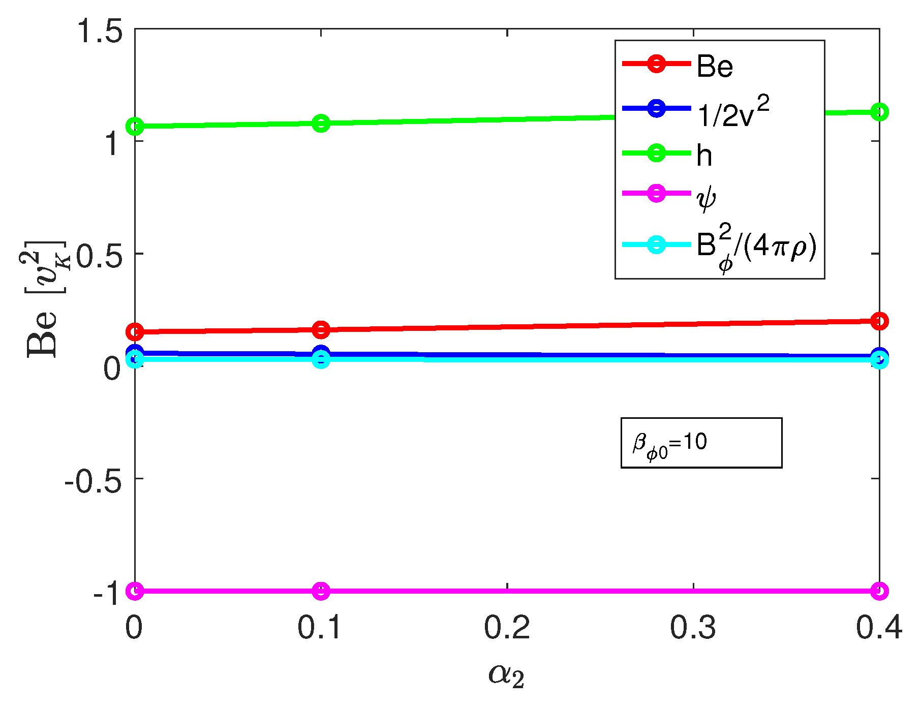
Figure 7 shows the Bernoulli parameter. Same as in the model with a weak magnetic field, the enthalpy dominates the kinetic and magnetic terms. The Bernoulli parameter increases in the presence of anisotropic pressure.
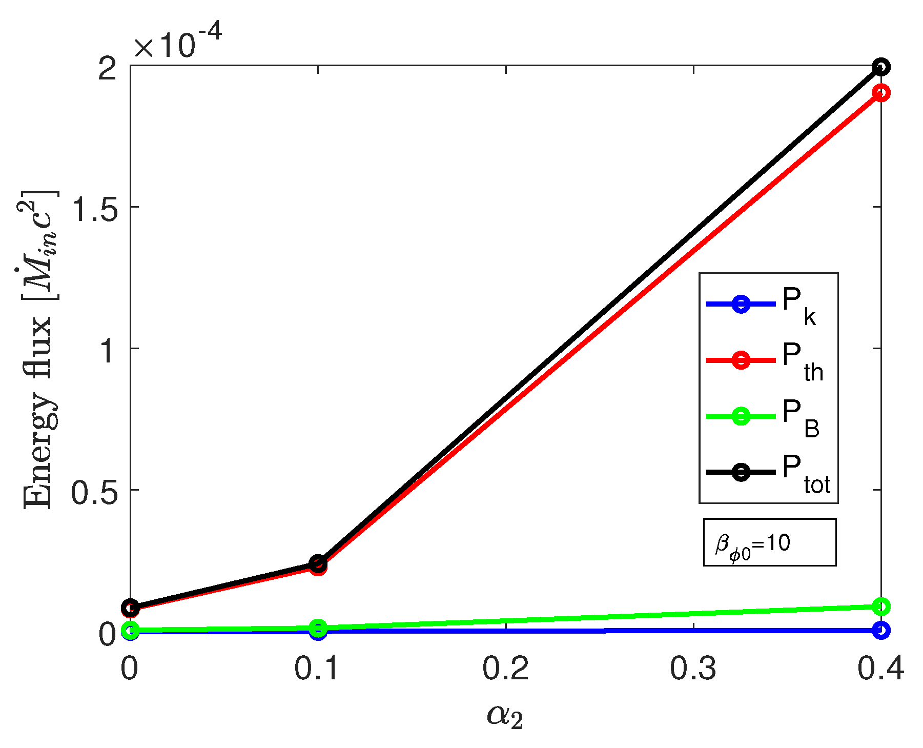
Figure 8 shows the energy fluxes carried by outflow. The thermal energy flux is much higher than the kinetic and Poynting energy fluxes. The work done by anisotropic pressure increases gas temperature. Correspondingly, the thermal energy flux carried by outflow increases significantly in the presence of anisotropic pressure. When , the total outflow power is 20 times higher than that when .
The mass outflow rate is about 70% of the mass inflow rate in the relatively strong magnetic case. The wind is powerful. Magnetohydrodynamic (MHD) simulation found that wind is driven by the combination of gas pressure gradient, magnetic pressure gradient, and centrifugal forces ([48]). When performing a stronger magnetic field, a stronger wind is driven.
For direct comparison, we plot a figure ( see Figure 9) with three different magnetic fields () change with a fixed anisotropic pressure . We can see when the magnetic field is stronger, and the outflow velocity turns to be larger than in a weak field case. Therefore, a stronger wind is performed. In both present works and [87], it is found that the value of decreases with the decrease of . has the largest value at the midplane. In [26] ( the simulations are about hot accretion flow), it is found that at midplane, is slightly larger than 1 (at the midplane gas pressure dominates magnetic pressure). Please note that at small region, [26] also found that can be smaller than 1. Both [87,95] are about the cold thin disc. They also found that the value of is largest at the midplane. In [87], at the midplane, the lowest value of is 0.4 (see Figure 1 in their paper). The value of at midplane for hot accretion flow ([26]) is different from that at the midplane for cold thin discs ([87]). The difference may be due to different physical conditions. We have tried to calculate the case at the midplane (we expect at the region , the value of beta can be much smaller than 0.1). We cannot obtain a solution. The reason may be that for hot accretion flow, the value of at midplane is required to be larger than 1.
4. Summary and Discussion
In extreme low-accretion-rate hot accretion flow, the collision of the ion means free path can be much larger than its Larmor radius. Pressure parallel to the magnetic field line is different from that perpendicular to the magnetic field line. We study the effects of anisotropic pressure on the properties of the hot accretion flow. In particular, we pay attention to how the outflow properties change with the strength of anisotropic pressure. The anisotropic pressure is modeled by the anisotropic viscosity. In the outflow region, the pressure is also anisotropic. Therefore, we still have a viscosity in an outflow far from the disk. We solve two-dimensional magnetohydrodynamic equations of hot accretion flow by assuming the flow is radially self-similar. We assume that the magnetic field only has a toroidal component. We find that the work done by anisotropic pressure can heat the flow and increases gas temperature. The Bernoulli parameter changes slightly when anisotropic pressure is included. However, the specific energy flux carried by outflow can be increased by a factor of 20. We found that with the increase of , the specific power of outflow increases. The value of depends on the accretion rate. Lower accretion rate system has lower particle collisional rate and higher value of . Therefor for hot accretion flow, the fraction of energy taken away from the accretion system by outflow increase with the decrease of accretion rate. Lower accretion rate system tends to drive stronger outflow/jet. The outflow feedback effects can be enhanced significantly in the presence of anisotropic pressure.
The black hole at the galactic center is believed to co-evolve with its host galaxy. AGN feedback plays a vital role in affecting the properties of its host galaxy. AGN outflow can interact with the interstellar medium significantly. The efficiency of interaction depends on the power of outflow. In this paper, we find that when considering anisotropic pressure, the power of outflow can be increased by a factor of ∼10. Therefore, AGN feedback effects can be significantly enhanced by the presence of anisotropic pressure.
Reference [82] assumed an extremely weak magnetic field. Consequently, their mass flow of outflow is quite weak; the mass inflow flow is ten percent of the out-mass flow. In our paper, when we assume a relatively stronger magnetic field (the gas pressure is 1000 times larger than the magnetic field), the outflow rate is quite large (the mass flux of outflow is 26% of inflow). When the gas pressure is ten times larger than the magnetic field, strong winds are formed. The mass outflow is about 70% to the mass inflow rate.
In this paper, the magnetic field is assumed only to have a toroidal component. In this case, the force due to the anisotropic pressure only exists in the radial and momentum equations. The presence of anisotropic pressure cannot transfer angular momentum. In reality, the vertical component of the magnetic field should also be present. When the poloidal component of the magnetic field is present, wind/jet can be formed ([48]). The convective motions of accretion flow can be suppressed ([24,26]). Since hydrodynamical simulations of hot accretion flow ([10]) found that if the magnetic field is absent, the accretion flow is kinetically unstable, convective motions are present. Plus, numerical simulations found that if the magnetic field is present, the convective motions disappears ([24,26]), the turbulent motion of accretion flow is induced by MRI. Lacking the presence of poloidal magnetic field may lead us to unrealistic results.
However, we think our results are trustable. For example, in our calculation, the outflow power increases when the anisotropic pressure increases. We find that the thermal energy flux of outflow is significantly higher than the kinetic energy flux of outflow. The anisotropic pressure plays a heating role. Therefore, with the increase of anisotropic pressure (), the temperature of outflow increases (see the bottom right panel of Figure 1 and Figure 5). Thus, the (thermal) power of outflow increases with the increase of . If a vertical magnetic field is present, the outflow should be stronger. The anisotropic pressure can still play a heating role in the presence of a vertical magnetic field. Therefore, with the increase of anisotropic pressure, the outflow temperature can still increase in the presence of the vertical magnetic field. We expect the (thermal) power of outflow can increase with the increase of anisotropic pressure even with the presence of the vertical magnetic field.
In the future, it is indispensable to perform numerical simulations, including all three components of the magnetic field to study the effects of anisotropic pressure on the dynamics of the hot accretion flow.
Author Contributions
D.-F.B. is the corresponding author, who supplies the idea of this paper. H.-H.D. is responsible for the calculations, plotting figures, writing—original draft, and writing—review & editing.
Funding
: This work is supported in part by the Natural Science Foundation of China (Grants 11773053, 11573051, 11633006, and 11661161012), the Key Research Program of Frontier Sciences of CAS (No. QYZDJSSW-SYS008).
Acknowledgments
We thank Amin Mosallanezhad for his helpful discussions. This work made use of the High-Performance Computing Resource in the Core Facility for Advanced Research Computing at Shanghai Astronomical Observatory.
Conflicts of Interest
The authors declare no conflict of interest. The funders had no role in the design of the study; in the collection, analyses, or interpretation of data; in the writing of the manuscript, or in the decision to publish the results.
References
- Blandford, R.; Payne, D.G. Hydromagnetic flows from accretion discs and the production of radio jets. Mon. Not. R. Astron. Soc. 1982, 199, 883–903. [Google Scholar] [CrossRef] [Green Version]
- Ferreira, J.; Pelletier, G. Low Mass Star Formation—From Infall to Outflow, Poster Proceedings of IAU Symp. No. 182; Malbet, F., Castets, A., Eds.; Observatoire de Grenoble: Chamonix, France, 1997; p. 112. [Google Scholar]
- Stepanovs, S.; Fendt, C. An extensive numerical survey of the correlation between outflow dynamics and accretion disk magnetization. Astrophys. J. 2016, 825, 14. [Google Scholar] [CrossRef]
- Murphy, G.C.; Ferreira, J.; Zanni, C. Large scale magnetic fields in viscous resistive accretion disks-I. Ejection from weakly magnetized disks. Astron. Astrophys. 2010, 512, A82. [Google Scholar] [CrossRef]
- Sheikhnezami, S.; Fendt, C.; Porth, O.; Vaidya, B.; Ghanbari, J. Bipolar jets launched from magnetically diffusive accretion disks. I. ejection efficiency versus field strength and diffusivity. Astrophys. J. 2012, 757, 65. [Google Scholar] [CrossRef]
- Stepanovs, D.; Fendt, C.; Sheikhnezami, S. Modeling MHD accretion-ejection: Episodic ejections of jets triggered by a mean-field disk dynamo. Astrophys. J. 2014, 796, 29. [Google Scholar] [CrossRef]
- Ichimaru, S. Bimodal behavior of accretion disks-Theory and application to Cygnus X-1 transitions. Astrophys. J. 1977, 214, 840–855. [Google Scholar] [CrossRef]
- Rees, M.J.; Begelman, M.C.; Blandford, R.D.; Phinney, E.S. Ion-supported tori and the origion of radio jets. Nature 1982, 295, 17. [Google Scholar] [CrossRef]
- Narayan, R.; Yi, I. Advection-dominated accretion: A self-similar solution. Astrophys. J. 1994, 428, L13–L16. [Google Scholar] [CrossRef]
- Stone, J.M.; Pringle, J.E.; Begelman, M.C. Hydrodynamical non-radiative accretion flows in two dimensions. Mon. Not. R. Astron. Soc. 1999, 310, 1002–1016. [Google Scholar] [CrossRef] [Green Version]
- Igumenshchev, I.V.; Abramowicz, M.A. Rotating accretion flows around black holes: Convection and variability. Mon. Not. R. Astron. Soc. 1999, 303, 309–320. [Google Scholar] [CrossRef]
- Igumenshchev, I.V.; Abramowicz, M.A. Two-dimensional models of hydrodynamical accretion flows into black holes. Astrophys. J. 2000, 130, 463. [Google Scholar] [CrossRef]
- Hawley, J.F.; Balbus, S.A.; Stone, J.M. A magnetohydrodynamic nonradiative accretion flow in three dimensions. Astrophys. J. 2011, 554, L49. [Google Scholar] [CrossRef]
- Machida, M.; Matsumoto, R.; Mineshige, S. Convection-dominated, magnetized accretion flows into black holes. Publ. Astron. Soc. Jpn. 2001, 53, L1–L4. [Google Scholar] [CrossRef]
- Stone, J.M.; Pringle, J.E. Magnetohydrodynamical non-radiative accretion flows in two dimensions. Mon. Not. R. Astron. Soc. 2011, 322, 461–472. [Google Scholar] [CrossRef]
- Hawley, J.F.; Balbus, S.A. The dynamical structure of nonradiative black hole accretion flows. Astrophys. J. 2002, 573, 738. [Google Scholar] [CrossRef]
- De Villiers, J.P.; Hawley, J.F.; Krolik, J.H. Magnetically driven accretion flows in the Kerr metric. I. Models and overall structure. Astrophys. J. 2003, 599, 1238. [Google Scholar] [CrossRef]
- Pen, U.L.; Matzener, C.D.; Wong, S. The Fate of Nonradiative Magnetized Accretion Flows: Magnetically Frustrated Convection. Astrophys. J. 2003, 596, L207. [Google Scholar] [CrossRef]
- Beckwith, K.; Hawley, J.F.; Krolik, J.H. The influence of magnetic field geometry on the evolution of black hole accretion flows: Similar disks, drastically different jets. Astrophys. J. 2008, 678, 1180. [Google Scholar] [CrossRef]
- Pang, B.; Pen, U.-L.; Matzner, C.D.; Green, S.R.; Liebendorfer, M. Numerical parameter survey of non-radiative black hole accretion: Flow structure and variability of the rotation measure. Mon. Not. R. Astron. Soc. 2011, 415, 1228–1239. [Google Scholar] [CrossRef]
- Tchekhovskoy, A.; Narayan, R.; McKinney, J.C. Efficient generation of jets from magnetically arrested accretion on a rapidly spinning black hole. Mon. Not. R. Astron. Soc. 2011, 418, L79–L83. [Google Scholar] [CrossRef]
- Tchekhovskoy, A.; McKinney, J.C. Prograde and retrograde black holes: Whose jet is more powerful? Mon. Not. R. Astron. Soc. 2012, 423, L55–L59. [Google Scholar] [CrossRef]
- Yuan, F.; Wu, M.; Bu, D. Numerical simulation of hot accretion flows. I. A large radial dynamical range and the density profile of accretion flow. Astrophys. J. 2012, 761, 129. [Google Scholar] [CrossRef]
- Yuan, F.; Bu, D.; Wu, M. Numerical simulation of hot accretion flows. II. Nature, origin, and properties of outflows and their possible observational applications. Astrophys. J. 2012, 761, 130. [Google Scholar] [CrossRef]
- McKinney, J.; Tchekhovskoy, A.; Blandford, R. General relativistic magnetohydrodynamic simulations of magnetically choked accretion flows around black holes. Mon. Not. R. Astron. Soc. 2012, 423, 3083–3117. [Google Scholar] [CrossRef] [Green Version]
- Narayan, R.; Sadowski, A.; Penna, R.F.; Kulkarni, A.K. GRMHD simulations of magnetized advection-dominated accretion on a non-spinning black hole: Role of outflows. Mon. Not. R. Astron. Soc. 2010, 426, 3241–3259. [Google Scholar] [CrossRef]
- Li, J.; Ostriker, J.; Sunyaev, R. Rotating accretion flows: From infinity to the black hole. Astrophys. J. 2013, 767, 105. [Google Scholar] [CrossRef]
- Sadowski, A.; Narayan, R.; Penna, R.; Zhu, Y. Energy, momentum and mass outflows and feedback from thick accretion discs around rotating black holes. Mon. Not. R. Astron. Soc. 2013, 436, 3856–3874. [Google Scholar] [CrossRef]
- Ho, L.C. Nuclear activity in nearby galaxies. Annu. Rev. Astron. Astrophys. 2008, 46, 475–539. [Google Scholar] [CrossRef]
- Antonucci, R. A panchromatic review of thermal and nonthermal active galactic nuclei. Astron. Astrophys. Trans. 2012, 27, 557–602. [Google Scholar]
- Done, C. Accretion flows in Binaries and AGN. In Proceedings of the Suzaku-MAXI 2014: Expanding the Frontiers of the X-ray Universe, Matsuyama, Japan, 19–22 February 2014; p. 300. [Google Scholar]
- Esin, A.A.; McClintock, J.E.; Narayan, R. Advection-Dominated Accretion and the Spectral States of Black Hole X-ray Binaries: Application to Nova Muscae 1991. Astrophys. J. 1997, 489, 865–889. [Google Scholar] [CrossRef]
- Fender, R.P.; Belloni, T.M.; Gallo, E. Towards a unified model for black hole X-ray binary jets. Mon. Not. R. Astron. Soc. 2004, 355, 1105–1118. [Google Scholar] [CrossRef] [Green Version]
- Zdziarski, A.A.; Gierliński, M. Radiative processes, spectral states and variability of black-hole binaries. Prog. Theor. Phys. Suppl. 2004, 155, 99–119. [Google Scholar] [CrossRef]
- Narayan, R. Low-luminosity accretion in black hole X-ray binaries and active galactic nuclei. Astrophys. Space Sci. 2005, 300, 177–188. [Google Scholar] [CrossRef]
- Remillard, R.A.; McClintock, J.E. X-ray properties of black-hole binaries. Annu. Rev. Astron. Astrophys. 2006, 44, 49–92. [Google Scholar] [CrossRef]
- Narayan, R.; McClintock, J.E. Advection-dominated accretion and the black hole event horizon. New Astron. Rev. 2008, 51, 733–751. [Google Scholar] [CrossRef] [Green Version]
- Belloni, T.M. States and transitions in black hole binaries. In The Jet Paradigm—From Microquasars to Quasars; Springer: Berlin/Heidelberg, Germany, 2010; pp. 53–84. [Google Scholar]
- Wu, Q.; Cao, X.; Ho, L.C.; Wang, D. A physical link between jet formation and hot plasma in active galactic nuclei. Astrophys. J. 2013, 700, 31. [Google Scholar] [CrossRef]
- Yuan, F.; Narayan, R. Hot accretion flows around black holes. Annu. Rev. Astron. Astrophys. 2014, 52, 529–588. [Google Scholar] [CrossRef]
- Crenshaw, D.M.; Kraemer, S.B. Feedback from mass outflows in nearby active galactic nuclei. I. Ultraviolet and X-ray absorbers. Astrophys. J. 2012, 753, 75. [Google Scholar] [CrossRef]
- Tombesi, F.; Sambruna, J.N.; Reeves, J.N.; Braito, V.; Ballo, L.; Gofford, J.; Cappi, M.; Mushotzky, R.F. Discovery of ultra-fast outflows in a sample of broad-line radio galaxies observed with suzaku. Astrophys. J. 2010, 719, 700. [Google Scholar] [CrossRef]
- Tombesi, F.; Tazaki, F.; Mushotzky, R.F.; Ueda, Y.; Cappi, M.; Gofford, J.; Reeves, J.N.; Guainazzi, M. Ultrafast outflows in radio-loud active galactic nuclei. Mon. Not. R. Astron. Soc. 2014, 443, 2154–2182. [Google Scholar] [CrossRef] [Green Version]
- Wang, Q.D.; Nowak, M.A.; Markoff, S.B.; Baganoff, F.K.; Nayakshin, S.; Yuan, F.; Cuadra, J.; Davis, J.; Dexter, J.; Fabian, A.C.; et al. Dissecting X-ray–emitting gas around the center of our galaxy. Science 2013, 341, 981–983. [Google Scholar] [CrossRef] [PubMed]
- Cheung, E.; Bundy, K.; Cappellari, M.; Peirani, S.; Rujopakarn, W.; Westfall, K.; Yan, R.; Bershady, M.; Greene, J.E.; Heckman, T.M.; et al. Suppressing star formation in quiescent galaxies with supermassive black hole winds. Nature 2016, 533, 504. [Google Scholar] [CrossRef] [PubMed]
- Ma, M.; Roberts, S.R.; Li, Y.; Wang, Q.D. Spectral energy distribution of the inner accretion flow around Sgr A* - clue for a weak outflow in the innermost region. Mon. Not. R. Astron. Soc. 2019, 483, M5614. [Google Scholar] [CrossRef]
- Homan, J.; Neilson, J.; Allen, J.L.; Chakrabarty, D.; Fender, R.; Fridriksson, J.K.; Remillard, R.A.; Schulz, N. Evidence for simultaneous jets and disk winds in luminous low-mass X-ray binaries. Astrophys. J. 2016, 830, L5. [Google Scholar] [CrossRef]
- Yuan, F.; Gan, Z.; Narayan, R.; Sadowski, A.; Bu, D.; Bai, X. Numerical simulation of hot accretion flows. III. revisiting wind properties using the trajectory approach. Astrophys. J. 2015, 804, 101. [Google Scholar] [CrossRef]
- Bu, D.; Yuan, F.; Wu, M.; Cuadra, J. On the role of initial and boundary conditions in numerical simulations of accretion flows. Mon. Not. R. Astron. Soc. 2013, 434, 1692–1701. [Google Scholar] [CrossRef] [Green Version]
- Bu, D.; Yuan, F.; Gan, Z.; Yang, X. Hydrodynamical numerical simulation of wind production from black hole hot accretion flows at very large radii. Astrophys. J. 2016, 818, 83. [Google Scholar] [CrossRef]
- Bu, D.; Yuan, F.; Gan, Z.; Yang, X. Magnetohydrodynamic numerical simulation of wind production from hot accretion flows around black holes at very large radii. Astrophys. J. 2016, 823, 90. [Google Scholar] [CrossRef]
- Xie, F.; Yuan, F. The influences of outflow on the dynamics of inflow. Astrophys. J. 2008, 681, 499. [Google Scholar] [CrossRef]
- Li, S.L.; Cao, X.W. Global dynamics of advection-dominated accretion flows with magnetically driven outflow. Mon. Not. R. Astron. Soc. 2009, 400, L1734. [Google Scholar] [CrossRef]
- Li, S.L.; Cao, X.W. The kinetic power of jets magnetically accelerated from advection-dominated accretion flows in radio galaxies. Mon. Not. R. Astron. Soc. 2010, 405, L61. [Google Scholar] [CrossRef]
- Gu, W.M. Mechanism of Outflows in Accretion System: Advective Cooling Cannot Balance Viscous Heating? Astrophys. J. 2015, 799, 71. [Google Scholar] [CrossRef]
- Ghasemnezhad, M.; Abbassi, S. The influence of outflow and global magnetic field on the structure and spectrum of resistive CDAFs. Astrophys. Space Sci. 2016, 361, 372. [Google Scholar] [CrossRef] [Green Version]
- Ghasemnezhad, M.; Abbassi, S. The influence of large-scale magnetic field in the structure of supercritical accretion flow with outflow. Mon. Not. R. Astron. Soc. 2017, 469, 3307. [Google Scholar] [CrossRef]
- Bu, D.; Mosallanezhad, A. The effects of magnetic field strength on the properties of wind generated from hot accretion flow. Astron. Astrophys. 2018, 615, A35. [Google Scholar] [CrossRef] [Green Version]
- Ostriker, J.P.; Choi, E.; Ciotti, L.; Novak, G.S.; Proga, D. Momentum driving: Which physical processes dominate active galactic nucleus feedback? Astrophys. J. 2010, 722, 642. [Google Scholar] [CrossRef]
- Ciotti, L.; Ostriker, J.P.; Proga, D. Feedback from central black holes in elliptical galaxies. III. Models with both radiative and mechanical feedback. Astrophys. J. 2010, 717, 708. [Google Scholar] [CrossRef]
- Ciotti, L.; Pellegrini, S.; Negri, A.; Ostriker, J.P. The Effect of Agn Feedback on the Interstellar Medium of Early-Type Galaxies: 2D Hydrodynamical Simulations of the Low-Rotation Case. Astrophys. J. 2017, 835, 15. [Google Scholar] [CrossRef]
- Weinberger, R.; Springel, V.; Hernquist, L.; Pillepich, A.; Marinacci, F.; Pakmor, R.; Nelson, D.; Genel, S.; Vogelsberger, M.; Naiman, J.; et al. Simulating galaxy formation with black hole driven thermal and kinetic feedback. Mon. Not. R. Astron. Soc. 2017, 465, 3291–3308. [Google Scholar] [CrossRef]
- Weinberger, R.; Springel, V.; Pakmor, R.; Nelson, D.; Genel, S.; Pillepich, A.; Vogelsberger, M.; Marinacci, F.; Naiman, J.; Torrey, P.; et al. Supermassive black holes and their feedback effects in the IllustrisTNG simulation. Mon. Not. R. Astron. Soc. 2018, 479, 4056–4072. [Google Scholar] [CrossRef] [Green Version]
- Yuan, F.; Yoon, D.; Li, Y.; Gan, Z.M.; Ho, L.C.; Guo, F. Active galactic nucleus feedback in an elliptical galaxy with the most updated AGN physics. I. low angular momentum case. Astrophys. J. 2018, 857, 121. [Google Scholar] [CrossRef]
- Yoon, D.; Yuan, F.; Gan, Z.; Ostriker, J.P.; Li, Y.; Ciotti, L. Active galactic nucleus feedback in an elliptical galaxy with the most updated AGN physics. II. high angular momentum case. Astrophys. J. 2018, 864, 6. [Google Scholar] [CrossRef]
- Bu, D.; Yang, X. Quenching Black Hole Accretion by Active Galactic Nuclei Feedback. Astrophys. J. 2019, 871, 138B. [Google Scholar] [CrossRef]
- Tanaka, T.; Menou, K. Hot accretion with conduction: Spontaneous thermal outflows. Astrophys. J. 2006, 649, 345. [Google Scholar] [CrossRef]
- Johnson, B.M.; Quataert, E. The effects of thermal conduction on radiatively inefficient accretion flows. Astrophys. J. 2007, 660, 1273. [Google Scholar] [CrossRef]
- Chandra, M.; Gammie, C.F.; Foucart, F.; Quataert, E. An extended magnetohydrodynamics model for relativistic weakly collisional plasmas. Astrophys. J. 2015, 810, 162. [Google Scholar] [CrossRef]
- Foucart, F.; Chandra, M.; Gammie, C.F.; Quataert, E. Evolution of accretion discs around a kerr black hole using extended magnetohydrodynamics. Mon. Not. R. Astron. Soc. 2016, 456, 1332. [Google Scholar] [CrossRef]
- Kunz, M.W.; Schekochihin, A.A.; Stone, J.M. Firehose and mirror instabilities in a collisionless shearing plasma. Phys. Rev. Lett. 2014, 112, 205003. [Google Scholar] [CrossRef]
- Hellinger, P.; Trávníček, P.M. Proton temperature-anisotropy-driven instabilities in weakly collisional plasmas: Hybrid simulations. J. Plasma Phys. 2015, 81, 305810103. [Google Scholar] [CrossRef]
- Riquelme, M.A.; Mario, A.; Quataert, E.; Verscharen, D. Particle-in-cell simulations of continuously driven mirror and ion cyclotron instabilities in high beta astrophysical and heliospheric plasmas. Astrophys. J. 2015, 800, 27. [Google Scholar] [CrossRef]
- Sironi, L.; Narayan, R. Electron heating by the ion cyclotron instability in collisionless accretion flows. I. Compression-driven instabilities and the electron heating mechanism. Astrophys. J. 2015, 800, 88. [Google Scholar] [CrossRef]
- Parrish, I.J.; Stone, J.M. Saturation of the magnetothermal instability in three dimensions. Astrophys. J. 2007, 664, 135. [Google Scholar] [CrossRef]
- Sharma, P.; Quataert, E.; Stone, J.M. Spherical accretion with anisotropic thermal conduction. Mon. Not. R. Astron. Soc. 2008, 389, 1815–1827. [Google Scholar] [CrossRef] [Green Version]
- Bu, D.; Yuan, F.; Stone, J.M. Magnetothermal and magnetorotational instabilities in hot accretion flows. Mon. Not. R. Astron. Soc. 2011, 413, 2808. [Google Scholar] [CrossRef]
- Quataert, E. A dynamical model for hot gas in the Galactic center. Astrophys. J. 2004, 613, 322. [Google Scholar] [CrossRef]
- Bu, D.; Wu, M.; Yuan, Y. Effects of anisotropic thermal conduction on wind properties in hot accretion flow. Mon. Not. R. Astron. Soc. 2016, 459, 746. [Google Scholar] [CrossRef]
- Quataert, E.; Dorl, W.; Hammett, G.W. The Magnetorotational Instability in a Collisionless Plasma. Astrophys. J. 2002, 577, 524. [Google Scholar] [CrossRef]
- Sharma, P.; Hammett, G.W.; Quataert, E. Transition from collisionless to collisional magnetorotational instability. Astrophys. J. 2003, 596, 1121. [Google Scholar] [CrossRef]
- Wu, M.; Bu, D.; Gan, Z.; Yuan, Y. Hot accretion flow with anisotropic viscosity. Astrophys. J. 2017, 608, A114. [Google Scholar] [CrossRef] [Green Version]
- King, A.R.; Pringle, J.E.; Livio, M. Accretion disc viscosity: How big is alpha? Mon. Not. R. Astron. Soc. 2007, 376, 1740. [Google Scholar] [CrossRef]
- Bu, D.; Xu, P.; Zhu, B. Self-Similar Solution of Hot Accretion Flow with Anisotropic Pressure. Universe 2019, 5, 89. [Google Scholar] [CrossRef]
- Machida, M.; Hayashi, M.R.; Matsumoto, R. Global simulations of differentially rotating magnetized disks: Formation of low-ßfilaments and structured coronae. Astrophys. J. 2000, 532, L67. [Google Scholar] [CrossRef] [PubMed]
- Hirose, S.; Krolik, J.H.; De Villiers, J.P.; Hawley, J.H. Magnetically driven accretion flows in the Kerr metric. II. Structure of the magnetic field. Astrophys. J. 2004, 606, 1083. [Google Scholar] [CrossRef]
- Bai, X.N.; Stone, J.M. Local study of accretion disks with a strong vertical magnetic field: Magnetorotational instability and disk outflow. Astrophys. J. 2013, 767, 30. [Google Scholar] [CrossRef]
- Mosallanezhad, A.; Bu, D.; Yuan, F. Two-dimensional inflow-wind solution of black hole accretion with an evenly symmetric magnetic field. Mon. Not. R. Astron. Soc. 2016, 456, 2877–2884. [Google Scholar] [CrossRef]
- Braginskii, S.I. Transport processes in a plasma. Reviews of plasma physics. Rev. Plasma Phys. 1965, 1, 205. [Google Scholar]
- Balbus, S.A. Viscous shear instability in weakly magnetized, dilute plasmas. Astrophys. J. 2004, 616, 857. [Google Scholar] [CrossRef]
- Salvesen, G.; Simon, J.B.; Armitage, P.J.; Begelman, M.C. Accretion disc dynamo activity in local simulations spanning weak-to-strong net vertical magnetic flux regimes. Mon. Not. R. Astron. Soc. 2016, 457, 857–874. [Google Scholar] [CrossRef] [Green Version]
- Narayan, R.; Yi, I. Advection-dominated accretion: Self-similarity and bipolar outflows. Astrophys. J. 1995, 444, 231–243. [Google Scholar] [CrossRef]
- Xue, L.; Wang, J.-C. The Effect of Outflow on Advection-dominated Accretion. Astrophys. J. 2005, 623, 372. [Google Scholar] [CrossRef]
- Jiao, C.L.; Wu, X.B. On the structure of accretion disks with outflows. Astrophys. J. 2011, 733, 112. [Google Scholar] [CrossRef]
- Das, U.; Begelman, M.C.; Lesur, G. Instability in strongly magnetized accretion discs: A global perspective. Mon. Not. R. Astron. Soc. 2018, 473, 2791–2812. [Google Scholar] [CrossRef]
Figure 1.
Angular profiles of velocities (), density (), pressure (p), and temperature (). The blue, red, yellow lines correspond to parameters , respectively. In this model, we set the gas pressure is 1000 times larger than the magnetic pressure at the midplane.
Figure 1.
Angular profiles of velocities (), density (), pressure (p), and temperature (). The blue, red, yellow lines correspond to parameters , respectively. In this model, we set the gas pressure is 1000 times larger than the magnetic pressure at the midplane.

Figure 2.
The magnetic pressure (), the ratio of gas pressure to magnetic pressure (), Mach number (), and change with . The blue, red, and yellow lines correspond to , and , respectively. Here, the gas pressure is 10 times larger than the magnetic pressure at the midplane.
Figure 2.
The magnetic pressure (), the ratio of gas pressure to magnetic pressure (), Mach number (), and change with . The blue, red, and yellow lines correspond to , and , respectively. Here, the gas pressure is 10 times larger than the magnetic pressure at the midplane.

Figure 3.
Bernoulli parameter in unit of . Here, the gas pressure is 1000 times larger than the magnetic pressure at the midplane.
Figure 3.
Bernoulli parameter in unit of . Here, the gas pressure is 1000 times larger than the magnetic pressure at the midplane.

Figure 4.
Energy fluxes carried by outflow. Here, the gas pressure is 1000 times larger than the magnetic pressure at the midplane.
Figure 4.
Energy fluxes carried by outflow. Here, the gas pressure is 1000 times larger than the magnetic pressure at the midplane.

Figure 5.
Angular profiles of velocities (), density (), pressure (p), and temperature (). The blue, red, yellow lines correspond to parameters , respectively. In this model, we set the gas pressure is 10 times larger than the magnetic pressure at the midplane.
Figure 5.
Angular profiles of velocities (), density (), pressure (p), and temperature (). The blue, red, yellow lines correspond to parameters , respectively. In this model, we set the gas pressure is 10 times larger than the magnetic pressure at the midplane.

Figure 6.
The magnetic pressure (), the ratio of gas pressure to magnetic pressure (), Mach number (), and change with . Here, the gas pressure is 10 times larger than the magnetic pressure at the midplane.
Figure 6.
The magnetic pressure (), the ratio of gas pressure to magnetic pressure (), Mach number (), and change with . Here, the gas pressure is 10 times larger than the magnetic pressure at the midplane.

Figure 7.
Bernoulli parameter in unit of . Here the gas pressure is 10 times larger than the magnetic pressure at the midplane.
Figure 7.
Bernoulli parameter in unit of . Here the gas pressure is 10 times larger than the magnetic pressure at the midplane.

Figure 8.
Energy fluxes carried by outflow. Here the gas pressure is 10 times larger than the magnetic pressure at the midplane.
Figure 8.
Energy fluxes carried by outflow. Here the gas pressure is 10 times larger than the magnetic pressure at the midplane.

Figure 9.
Angular profiles of a variety of physical variables. The blue, red, green lines correspond to parameters , respectively. Here, set to be 0.1.
Figure 9.
Angular profiles of a variety of physical variables. The blue, red, green lines correspond to parameters , respectively. Here, set to be 0.1.

© 2019 by the authors. Licensee MDPI, Basel, Switzerland. This article is an open access article distributed under the terms and conditions of the Creative Commons Attribution (CC BY) license (http://creativecommons.org/licenses/by/4.0/).
Share and Cite
MDPI and ACS Style
Deng, H.-H.; Bu, D.-F. Hot Accretion Flow in Two-Dimensional Spherical Coordinates: Considering Pressure Anisotropy and Magnetic Field. Universe 2019, 5, 197. https://doi.org/10.3390/universe5090197
AMA Style
Deng H-H, Bu D-F. Hot Accretion Flow in Two-Dimensional Spherical Coordinates: Considering Pressure Anisotropy and Magnetic Field. Universe. 2019; 5(9):197. https://doi.org/10.3390/universe5090197
Chicago/Turabian StyleDeng, Hui-Hong, and De-Fu Bu. 2019. "Hot Accretion Flow in Two-Dimensional Spherical Coordinates: Considering Pressure Anisotropy and Magnetic Field" Universe 5, no. 9: 197. https://doi.org/10.3390/universe5090197
Note that from the first issue of 2016, this journal uses article numbers instead of page numbers. See further details here.