Abstract
The possibility of an equilibrium state of a gravitating scalar field (describing ordinary matter) inside a black hole, compressed to the state of boson condensate, in balance with a longitudinal vector field (describing dark matter) from the outside, is considered. Analytical analysis, confirmed numerically, shows that there are regular static solutions to the Einstein equations with no limitation on the mass of a black hole. The metric tensor component grr(r) changes sign twice. The behavior of the gravitational field and material fields in the vicinity of these two Schwarzschild radii were studied in detail. The equality of the energy–momentum tensors of the scalar and longitudinal vector fields at the interface supports the phase equilibrium of a black hole and dark matter. Considering the gravitating scalar field as an example, a possible internal structure of a black hole and its influence on the dark matter at the periphery of a galaxy are clarified. In particular, the speed on the plateau of a galaxy rotation curve as a function of a black hole’s mass is determined.
1. Introduction
Astrophysical observations indicate the existence of super-massive objects at the centers of galaxies. In our Milky Way, there is an invisible object located in the same place as the radio source “Sagittarius A”. According to the orbital motion of stars, astronomers estimate its mass to be 4.3 × 10⁶ Mʘ, and its radius to be less than 0.002 light years [1]. The mass of the Sun is Mʘ = 1.989 × 1033 g. If the mass of an object in the center of a galaxy is six orders of magnitude greater than the maximum equilibrium mass of a neutron star, then it is natural to consider black holes as the most likely candidates for super-massive objects in the centers of galaxies.
According to modern concepts, a black hole is a process of unlimited compression (collapse) of matter under the action of dominant forces from its own gravitational field. In this case, the density grows indefinitely, and the energy per particle inevitably reaches and exceeds the binding energy of “elementary” particles in neutrons, or in their composite components.
The time of existence of galaxies (and, consequently, of black holes in their centers) is of the order of lifetime of the universe. With a very slow evolution of a black hole, the local equilibrium concentrations of particles, transforming one into another via “chemical reactions”, depend on temperature and pressure, and do not depend on specific reaction channels (Reference [2], Section 101). One of the most important issues, that is not yet clarified, is the reverse effect of mutual transformations of particles on the process of gravitational self-compression. The fact that the lifetime of a galaxy with a collapsing object in the center is of the order of the universe’s lifetime suggests that the mutual transformation of particles one into another can slow down the compression process, or even stop it. This is the main reason for searching and analyzing static configurations of gravitating objects in the general theory of relativity.
In the macroscopic theory of dark sector [3], the contribution to the galaxy rotation curves by dark matter, described by a longitudinal vector field, is expressed in terms of the non-zero covariant divergence of the field at the center. is a free parameter of the theory [3]. In fact, the non-zero value depends on the interaction of dark matter with a black hole in the center of a galaxy. To establish this connection, it is necessary to analyze the internal structure of a black hole in balance with the dark matter outside of it. In a vacuum (with no stabilizing action by dark matter) an equilibrium state of a super-heavy black hole would be impossible.
In the process of gravitational collapse, the density of matter increases continuously. The stage of compression, when massive Bose particles (Z bosons, W bosons, Higgs scalar bosons, and/or boson pairs of fermions) are dominating, is inevitable. At low temperatures, a degenerate boson gas is energetically more favorite than a degenerate fermion gas. At zero temperature, bosons are located on the ground level. This state of boson matter is named Bose–Einstein condensate. Its wave function is a scalar field (Reference [4], Section 26). At the border of a super-massive scalar field, the energy density vanishes, but the pressure does not. If a degenerate Fermi gas is considered as the ordinary matter of a black hole, then both the energy density and pressure are zeros on the surface. Therefore, a realization of phase equilibrium on the interface of a super-massive black hole and dark matter is more likely at the stage of domination of boson matter in a collapsing black hole.
The main properties of a gravitating Bose–Einstein condensate in an equilibrium state are summarized in my review article [5], published in an issue of the Journal of Experimental and Theoretical Physics (JETP), dedicated to the 85th anniversary of academician Pitaevskii. Applying a homogeneous Klein–Gordon equation, we deal with a nonlinear eigenvalue problem. At a slightest deviation of parameters from eigenvalue, the integral curves go into the signature area of the opposite sign, which is tacitly considered to be “non-physical”. With a restriction of a constant signature, it is not possible to find static solutions that adequately describe the equilibrium state of gravitating super-massive objects.
A possible equilibrium structure of a gravitating scalar field in the region of space of a black hole with the signature changing sign (within the Schwarzschild sphere, where ) is considered in this article. Instead of representing the metric tensor component , which fixes the sign, I use a less rigorous condition of regularity. A change in the metric signature does not lead to logical contradictions, since it occurs beyond the event horizon in an inaccessible area to a remote observer.
The condition of phase equilibrium at the interface between a scalar field (black hole) and a longitudinal vector field (dark matter) determines the covariant divergence of the longitudinal vector field. It becomes possible to establish a connection between the plateau velocity of a galaxy rotation curve and the black hole’s mass (see Equation (68) below).
2. Space-Time, Strongly Curved Up to Changing the Signature of Metric Tensor
In the framework of the standard approach, a static space-time metric,
with a spherically symmetric distribution of matter, is considered.
In the general theory of relativity, one can introduce a local Galilean coordinate system at any point of a smoothly curved space-time. In a curved space-time, a transition from one coordinate system to another, and back, is unambiguous if the Jacobean j of transformation is non-zero. The Jacobean of a transition from coordinates to can be expressed in terms of the determinants of metric tensors and :
where (Reference [6], Section 83). The signature of a Galilean coordinate system is (+, −, −, −). The Jacobean of transition from Galilean coordinates , where , to curved ones is .
In our case of interest, the metric tensor in Equation (1) is diagonal, and there is a Schwarzschild’s sphere inside a gravitating object, where the component changes sign, while does not. When only changes sign, the signature of metric tensor (1) becomes (+, +, −, −). Accordingly, . On the Schwarzschild radius, the Jacobean . Due to different signatures on the opposite sides, the space-time can be either locally flat, or locally non-flat on the hyper-sphere .
Formally, derivation of Einstein equations at , and at should be carried out separately, with where , and in the area with . For both sides, the static gravitational field, created by a spherically symmetric distribution of matter, satisfies the same Einstein equations (see Equations (100.4) and (100.6) in Reference [6]). We write them down in the following form:
Gravitational constant , , .
The general solution of Equation (3) is
r0 is a constant of integration, and is a regular function, provided that the integral in Equation (5) converges. The convergence of this integral means that the mass within the layer ,
(with account of gravitational mass-defect) is finite. If the total mass is finite, the metric component is a continuous function within the whole space . The regularity of follows from the finiteness of the total mass of matter, regardless of its physical nature.
A static solution to Einstein’s equations for a gravitating point-size body was found by Schwarzschild back in 1916 [7].
Actually Equation (7) is applicable outside a gravitating body, including its boundary, provided that, on the surface, . At Newton’s law is applicable, and the Schwarzschild radius is proportional to the total mass M of a gravitating point-like object in the center.
In a vacuum, outside a gravitating body, there is no physical reason for the existence of irregularities. Naturally, the determinant of a Schwarzschild’s static metric (Equation (100.14) in Reference [6]), as well as the determinant of a stationary Kerr’s metric (Equation (104.2) in Reference [6]), does not change signs. In a vacuum, metric signatures remain unchanged, and the space-time on the hyper-surface is locally flat.
Analyzing the equilibrium states of spherically symmetric gravitating matter, it is usually assumed that the energy density at the center is finite, and the metric tends to the Galilean metric at infinity. Bearing in mind a regular solution in the whole space, people choose two equations,
as boundary conditions for the Einstein Equations (3) and (4). These kinds of solutions exist only if the total mass of matter does not exceed a critical value . Critical mass is of the order of the Sun mass in case of a degenerate neutron Fermi gas. For a Bose–Einstein condensate (see Reference [5]),
Plank mass . For bosons with a mass , the critical mass is about one million tons. In the solutions with boundary conditions from Equation (9) and total mass , the metric component does not change sign at all.
Formally, at the absolute zero temperature in a vacuum, there could exist static states of boson condensate having an arbitrarily large mass with not changing sign. However, these states are metastable. An aggregate of numerous isolated centers, each containing a condensate with the maximum possible mass of the order of Equation (10), is energetically more advantageous [5].
As applied to the gravitating Bose–Einstein condensate, the Klein–Gordon Equation (16) for the condensate wave function, together with Einstein Equations (3) and (4), form a complete set of equations. Equation (16) is a homogeneous second-order equation. We face a nonlinear eigenvalue problem [5]. If the total mass M is less than the critical , then, starting from −1, the function grows with increasing r, achieves its maximum value, and decreases back to −1 as . With the function remains negative within the whole interval .
At the slightest deviation from an eigenvalue, the integral curve grows monotonically and inevitably changes sign at some . Note that . If the total mass , then the integral in Equation (6) converges at the upper limit, and the energy density decreases faster than r−3 as . Looking at Equation (3), one can see that, in the region of changed signature , the derivative (grr)′ becomes negative when (1 + grr)/r exceeds with growing r. It means, that there may exist (and does exist, see below) a solution where, with increasing r, the metric component gets into the region of violated signature, passes through a maximum, and returns back into the region of the Galilean signature. intersects the x-axis twice.
Suppose that the metric signature is changed to (+, +, −, −) within a spherical layer . Then,
If , then and the Jacobean in Equation (2) are zeros at , and at . The area of the modified metric signature is tacitly considered “non-physical”. I do not see a reason why (unlike the Schwarzschild’s and/or Kerr’s metrics in a vacuum) a super-massive gravitating object cannot curve the space-time very strongly, up to changing the signature of the metric tensor inside a material medium.
Yes, there can exist selected regions, like hyper-spheres and , where space-time is not locally flat. As a rule, it happens, if there is a physical reason. In our case, the radial function of the gravitating Bose–Einstein condensate satisfies the Klein–Gordon Equation (19). is the coefficient at the highest derivative. At , Equation (19) is not defined, since the coefficient at the highest derivative is zero. I used a standard approach to the problem of a small parameter at the highest derivative in Section 3.
From the general solution in Equation (5) to Equation (3), we get the identity
If, in the region , the metric signature (+, −, −, −) remains unchanged, then is the event horizon for a remote observer. In the Schwarzschild solution in Equation (7), turning to zero can happen at any radius outside the gravitating body. However, in a vacuum, the determinant of metric tensor is non-zero, and the metric signature remains unchanged. Turning to zero, followed by the change of the metric signature, can take place inside a body, or on its surface, or on the interface of two gravitating objects.
As it follows from the identity in Equation (12), in the presence of a layer with a different signature, the radius is not connected with the whole mass of a gravitating object, but only with its part inside the layer. The total mass M is connected with the horizon by Equation (8) only if the integral in Equation (12) converges at . In this case the relation in Equation (7) takes place for . At , we have
In view of Equation (13), it follows from Einstein Equations (3) and (4) that
Turning the energy density to zero at means that the surface of a gravitating body can be an event horizon. However, since , the pressure on the surface does not disappear. It means that (without taking into account interactions of a non-gravitational nature) there can be no static equilibrium state of a gravitating body in a vacuum with a broken signature of the metric tensor. Nevertheless, one cannot exclude a possibility that the event horizon takes place on the interface between two gravitating objects, for instance, if the inside pressure of a black hole is balanced by the pressure of dark matter from outside.
According to modern concepts, the amount of dark matter in the universe is several times larger than the amount of the ordinary (baryonic) matter. The presence of dark matter opens up a possibility for existence of static solutions to the Einstein equations describing the gravitational field of spherically symmetric matter with no limitation of mass. An example of such a solution, in which the metric component changes sign twice (firstly, inside a black hole and, secondly, on the interface with dark matter), is investigated below. The equilibrium state of a super heavy black hole becomes possible due to the presence of dark matter. The balance of pressures at the interface of a black hole and dark matter is able to support a static equilibrium of these two phases. Let us demonstrate this considering a gravitating scalar field as an example of ordinary (not dark) matter inside a black hole.
3. Gravitating Scalar Field behind the Horizon
The Lagrangian of a complex scalar field ψ in a curved space-time with the metric tensor (Equation (1)) has the form
In accordance with the least action principle, ψ and ψ* satisfy the Klein–Gordon equation.
From the point of view of equilibrium in its own gravitational field, it is implied that the number of quanta of the field is large, and all interactions, except the gravitational one, are not significant. Today, the interaction of dark and ordinary matter is observed through the curvature of space-time only.
The main characteristic determining the gravitational properties of a scalar field is the mass of a quantum m. In the power series of the potential,
term and higher degrees are corrections for collisions of particles and/or interactions of non-gravitational nature. Omitting these corrections, in Equation (16) is a constant having the dimension cm−2. It is related to the mass of the quantum m: .
Time is a cyclic coordinate in a static field. The energy of a single quantum E = ω is the integral of motion. In a flat space-time, the Klein–Gordon Equation (16) is a linear one. Its solution is a plane wave , describing the motion of a particle with relativistic spectrum . In a curved space-time, E is the conserved energy of the field per one quantum. A scalar field in the state of definite energy E has the form
Radial function ψ(r) obeys the equation
Note that is the coefficient at the highest derivative in Equation (19). Since , the Klein–Gordon equation is not determined on the hyper-sphere .
The Lagrangian (15) of a scalar field does not depend on the derivatives of the metric tensor. The energy–momentum tensor is derived by the formula
For the components of the mixed energy–momentum tensor, operating in the Einstein Equations (3) and (4), we find
The relation
follows from Equation (21). Using the relations in Equations (21) and (22), it is convenient to present the set of field and Einstein Equations (19), (3) and (4) in the normal form. In the dimensionless variables ,
we have a system of four first-order equations, resolved with respect to derivatives:
The set of Equations (24)–(27) contains no parameters. In Equation (23) and below, g(x) is the component of the metric tensor. Please do not confuse it with the determinant in the previous formulas.
Denote a dimensionless gravitational radius . At the component of metric tensor . Equations (24)–(27) are determined at , and at separately. They are not determined at because, at this point, the coefficient at the highest derivative in the scalar field Equation (19) is zero.
It follows from Equation (27) that, at , (+0 means from above, and −0 means from below)
Here, and are one-sided limits either from above or from below. Substituting Equation (28) into Equation (26), we obtain:
Note that the derivative does not depend on the behavior of and at . The assumption of linearity for at is not required in advance. The linearity of at follows directly from Equation (3) provided that is a regular function. Energy density is a continuous function inside a homogeneous medium and, therefore, one can put in Equation (29).
The sign of depends on the difference . If , then the function itself , and its derivative at . If , the derivative and is a growing function in the vicinity of . In the case , we have , and is a decreasing function in the vicinity of the horizon .
It follows from Equations (28) and (29) that
On the left-hand side ; thus, the right-hand side of Equation (30) is also a positive quantity. The derivative in Equation (29) is a non-zero constant. The factor in Equation (30) changes sign at . Therefore, the combination has different signs at and . In the case when Equation (30) makes sense if at , and at .
3.1. Regular Gravitational Radius
In the case of exact connection between the parameters,
all four functions, , as well as their derivatives, are continuous at . In accordance with Equation (28), at . From Equations (25) and (27), we find
With the exact connection in Equation (31), we have a regular solution of Equations (24)–(27), continuous on the boundary between the regions of different signatures of the metric tensor:
It is convenient to use these relations as boundary conditions for numerical integration. There are two free dimensionless parameters and .
In the absence of the relation in Equation (31), function h(x) would have a gap at . Without a physical reason, just like in a vacuum, there should be no discontinuity of the metric component inside a homogeneous medium.
3.2. Horizon
A sphere, where and , can be the surface of a gravitating body. In this case, at . The scalar field terminates at in a square-root manner. It is the event horizon for a remote observer. In order to avoid confusion, the event horizon where w(x) tends to zero as a square root we denote . We leave the notation for a regular gravitational radius inside a black hole. The horizon with a root feature is the upper border of the region occupied by the scalar field.
Solutions with the metric function g(x), changing signs twice deserve attention: once inside a black hole at a regular gravitational radius and the second time at the horizon .
The area is a layer with a violated signature of the metric tensor. is positive in this zone. Intervals and , where the metric function , are ordinary space-like zones. In the region (from the center to the horizon ) the scalar field is a regular function of the radius. In this region, the unknowns satisfy Equations (24)–(27) with the boundary conditions in Equation (33) in the close vicinity of .
At the boundary of the scalar field, the energy density vanishes (Equation (14)). Comparing in Equation (13) with Equation (29), valid for both cases and , we find that, at the termination point (on the horizon ), the scalar field is non-zero: . In the vicinity of the horizon, we get
The series expansion near the horizon goes in powers of . Determining and at from Equation (27), we see that the main contribution comes from the combination . In accordance with Equation (28), . The main term of expansion is
Inside the horizon sphere the derivative (see Equation (35)). If a test body is at rest, then the force acting on it is directed toward the center (Reference [6], problem 1 at the end of Section 88).
4. Numerical Analysis
4.1. Strip of Regular Solutions
Numerical analysis confirms that, in accordance with Equation (32), within the area of parameters,
there are finite-mass solutions, continuous at the regular gravitational radius , and terminating in a root manner at the horizon . These solutions are of physical interest. In the plane of parameters (), the region in Equation (36) is the strip between blue and red lines in Figure 1.
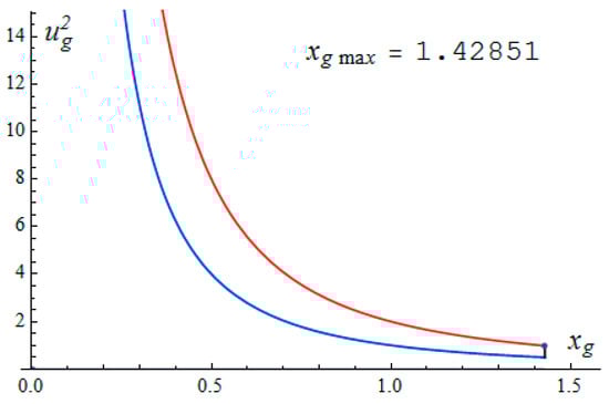
Figure 1.
The blue line in the plane of parameters (Equation (36)) is the lower boundary of the area of existence of regular solutions with finite mass M. The denominator of (Equation (32)) is zero on the blue line. The red line is the upper limit. At , the total mass . (Equation (32)) is zero on the red line.
On the bottom blue line, . On the upper red line, . If the parameters and in the boundary conditions in Equation (33) are inside the strip between the blue and red lines in Figure 1, then the corresponding solution to Equations (24)–(27) is regular and smooth in the domain , including the interval with the violated signature of the metric tensor.
4.2. Example of a Regular Solution behind the Horizon
An example of a regular solution is shown in Figure 2.
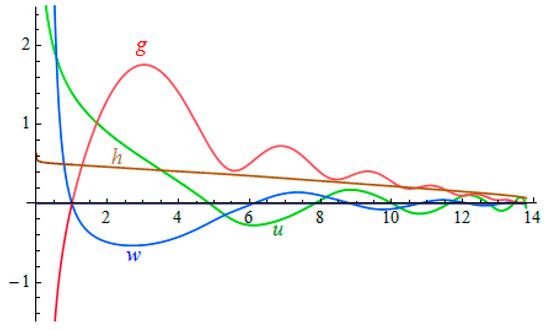
Figure 2.
An example of a regular solution to the set of Equations (24)–(27) with boundary conditions in Equation (33). . In accordance with Equation (31), The horizon radius is found numerically.
On the interval , the metric component . This is the region of changed signature. Its left (regular) boundary is . On the right boundary , the scalar field u(x) terminates with a non-zero value. On enlarged scales, this solution in the vicinity of the horizon is shown in Figure 3.
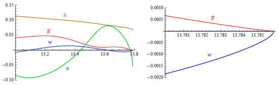
Figure 3.
The same functions and h(x), as in Figure 2, near (left graph), and very close to the horizon (right graph).
The wave function u(x) (green line) terminates at the horizon with a non-zero value and a root feature. In the very close vicinity of (Figure 3, right graph), one can see that w(x) (blue line) vanishes at in a square-root form.
4.3. In the Vicinity of the Upper Boundary
The behavior of all four functions in the vicinity of the upper boundary of the strip in Equation (36) is presented in Figure 4.
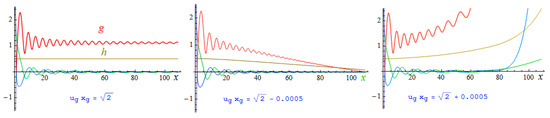
Figure 4.
Functions u(x) green, w(x) blue, g(x) red, and h(x) brown in the vicinity of the upper border of the strip in Equation (36).
At the border (Figure 4, left graph), g(x) tends to a constant value through damping oscillations. Below the border, the horizon radius and total mass M are finite. An example is shown in Figure 4, middle graph: the horizon Above the upper boundary of the strip in Equation (36) ( see Figure 4, right graph), there are no configurations with a finite mass M.
The band of existence of regular solutions in the plane () has a restriction from the right: This limitation is due to the fact that, at , the first left minimum of the red curve g(x) in Figure 5 touches the horizontal axis at the point x = 2.87. After that, g(x) remains positive and grows indefinitely with x.
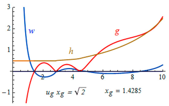
Figure 5.
Functions on the right boundary of the regularity domain in Equation (36). .
4.4. Core of a Black Hole
In the domain , the metric component The dimensionless scalar field diverges logarithmically as .
It is clear from Figure 6a, where (dashed green line) terminates at with a constant value depending on the product . Dependence is shown in Figure 6b.
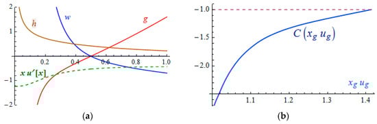
Figure 6.
Dashed green line is (a). Dependence (Equation (37)) (b).
The logarithmic divergence of the wave function in the center takes place because, in view of dominating gravity, interactions of other physical natures are not taken into account. At zero temperature in a static state, the equilibrium concentration of particles involved in the processes of decay and synthesis depends on pressure and does not depend on the specific reaction channel (Reference [2], Section 101). In particular, we ignored the fact that, in “chemical” reactions, the equilibrium concentration of bosons of the standard model falls down in the limits of very low and extremely high density. It is highly likely that this circumstance “cuts off” the logarithm in Equation (37) so that the wave function of bosons in the center becomes finite. In this case, the mass (inside the regular gravitational radius ) also remains finite. However, the contribution of to the total mass is not determined by the value of because of the large logarithm, whose value depends on the non-gravitational interactions of particles.
Corrections caused by non-gravitational interactions can be taken into account using the term in the power series of the potential in Equation (17). It is argued in the article [8] that an equilibrium configuration (with no signature changing) can differ significantly from the case of non-interacting bosons, even when λ is a small parameter. The analysis of the role of non-gravitational interaction of bosons in the strongly compressed state is beyond the scope of this article.
According to the identity in Equation (12), the mass (Equation (6)) in the layer between the regular gravitational radius and the horizon is
The internal gravitational radius (in units of the de Broglie wavelength of a boson) is of the order of unity and less. The gravitational radius of a black hole is larger, and even much larger, than the gravitational radius of the Sun. Although the inequality has a large margin, a remote observer does not determine the total mass of a black hole from the Newtonian asymptote
He (or she) determines only the almost total mass. The core mass of a black hole remains unknown to a distant observer. Although the core mass may be quite large due to the logarithmic divergence, it does not affect the asymptote in Equation (39).
The possibility of existence of a partially hidden mass within a collapsed black hole is associated with an extremely strong curving of space-time, up to violation of the metric signature. This can be treated as a variant of gravitational mass defect. In this regard, it is appropriate to recall Andreev’s prediction back in 1973 about the possible existence of macroscopic objects, whose mass is zero due to the gravitational mass defect [9].
The behavior of the metric function (red lines) at three decreasing values of (0.1, 0.01, and 0.001) with simultaneous increasing along the trajectory,
is shown in Figure 7A–C.
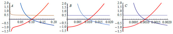
Figure 7.
Red lines in graphs A, B, and C show that, with a decrease of (and a simultaneous increase of along the path in Equation (40)), the metric function gets closer to −1 in the center. Values of are 0.1 (A), 0.01 (B), and 0.001 (C). The blue line is , and the brown line is .
Total mass increases sharply with a decreasing . In a regular center . In this case, the ratio of the circumference to diameter tends to π at . One can see that decreases with the growth of total mass, and as the metric function gets closer to −1. The larger the mass of a black hole is, the less significant the logarithmic singularity in the center will be.
4.5. Super-Heavy Black Hole
The greater the mass of a black hole is, the higher its density will be, and the smaller the size of the core in the center will be. In other words, for a fixed value of the product , the horizon radius increases sharply with a decrease of internal regular gravitational radius . The dependence at (along the dashed line in Figure 8b) is shown in Figure 8a.
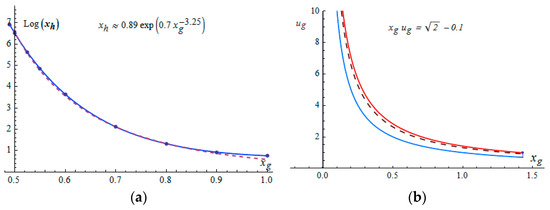
Figure 8.
Dependence (a) along the dashed line (b).
The solid line in Figure 8a is the interpolation of the numerically found points. A barely noticeable dashed line is the approximation by the formula
By reducing by half (along the dashed line in Figure 8b), the horizon (together with the mass ) increases by six orders of magnitude (see Figure 8a). Also, by increasing at a fixed value of , the horizon and mass grow and become infinitely large when approaches the upper red border in Figure 1 (and/or Figure 8b). The zone of a violated metric signature inside a black hole makes the existence of super-heavy objects (with no limitation of mass) possible.
As an example of a massive scalar field, the metric function g(x) for and (close to the upper border of the regularity strip) is shown in Figure 9.
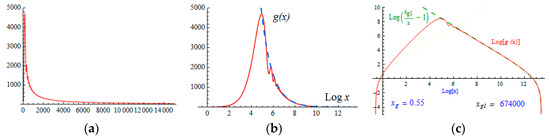
Figure 9.
Metric function g(x): (a) linear scale, (b) log(x) scale, (c) double-log scale.
With these parameters, the horizon is It is much farther than the end of the horizontal axis in Figure 9a. In order to see how the part of the graph that “stuck” to the vertical axis looks like, the same function g(x) is presented in Figure 9b with a logarithmic scale along the x-axis. The dashed line in Figure 9b is the Schwarzschild’s asymptote outside the gravitating mass extrapolated back into the region of localization of the scalar field. The same graph g(x) is shown in Figure 9c with logarithmic scales along both axes. It clearly demonstrates the relationship between and .
The dimensionless metric function h(x) decreases monotonically in the interval (,). Moreover, the longer the interval (,) is, the sharper h(x) decreases. With the same parameters and , as in Figure 9, the function h(x) almost disappears at the horizon . h(x) does not change sign up to (see Figure 10). Extrapolation to the termination point gives the estimate .
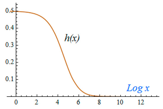
Figure 10.
Function h(x) in the interval (,) of broken signature. , .
According to Equation (34), . In the above example (, ), the amplitude of the scalar field at the horizon is .
Components of the energy–momentum tensor in Equation (21), expressed in terms of dimensionless variables in Equation (23), are as follows:
By virtue of Equations (28) and (34), the energy density of a scalar field vanishes at the horizon: . The pressure at the horizon is non-zero. In accordance with Equation (21) and following Equations (34), (42), and (28), we have
The pressure at the horizon in Equation (43) is inversely proportional to the square of the mass. For a black hole with the visible mass of the order of solar mass Mʘ = 2 × 1033 g, the component of the energy–momentum tensor g/(cm × sec2), that is, atmospheres. A static gravitating scalar field with a very high uncompensated pressure on the interface with a vacuum cannot exist. But this is without dark matter. The presence of dark matter outside the gravitating scalar field makes it possible to ensure a pressure balance at the interface of these two media.
5. Longitudinal Vector Field
The wave function of Bose–Einstein condensate, being a scalar, satisfies the Klein–Gordon Equation (16). Its derivative is a covariant vector. In the case of a longitudinal vector field, it is the opposite situation. The wave function is a vector, and its covariant divergence , being a scalar, satisfies the Klein–Gordon Equation (16). At the same time, the wave function itself is a gradient of the scalar [3],
The mass of a quantum of a longitudinal vector field is denoted by μ, so as not to be confused with the mass m of a quantum of a scalar field. A longitudinal vector field has a potential. The covariant derivative of the field is its potential at the same time.
Lagrangian of a longitudinal vector field ,
depends on the derivatives of the metric tensor via . The energy–momentum tensor is derived using the general Equation (94.4) in Reference [6]. The detailed derivation of the energy–momentum tensor of a longitudinal vector field,
is given in Reference [3] (Section 2.4).
For a super-heavy black hole, the inequality >> is carried out with a huge margin. The function h(x) at is negligible in comparison with unity. One can see it in Figure 10. Energy–momentum tensors in Equations (21) and (46) have the same structure on the interface region. Only the wave function and the derivative are swapped, and masses of quanta are different. In dimensionless variables with as a unit of length,
we have the following system of equations describing the longitudinal vector field and the gravitational field outside a black hole
Equations (48)–(51) are similar to Equations (24)–(27), presented in Section 3 in the reference frame with as a unit of length. Doing the same derivations as in Section 3, we get the derivative of the metric function at the interface from the side of dark matter:
Equations (52) and (29) are derived in different reference systems. Turning from Equation (47) to the reference system used inside a black hole (Equation (23)),
we see that Equation (52) is invariant against this transformation:
Regularity of the gravitational field means that the metric function and its derivative are continuous at the horizon . From Equations (29), (54), and (34), it follows that
In this case, the components of the energy–momentum tensors of the scalar and vector fields coincide at the interface
The equality in Equation (55) provides the balance of pressures on both sides of the horizon . This is the phase equilibrium of the scalar field inside the horizon, and the longitudinal vector field describing dark matter outside the horizon.
6. Galaxy Rotation Curve: Dependence of Plateau Velocity on the Mass of a Black Hole
In Equations (24)–(27), the unit of length along the x-axis is the de Broglie wavelength of a quantum of the scalar field (~10−16 cm for a quantum with the rest mass ~ 100 GeV/c2). The argument of covariant divergence and other functions in Equations (48)–(51) is . On the galactic scale, a natural unit of length is the de Broglie wavelength of a quantum of the longitudinal vector field. According to damped oscillations on the plateau of galaxy rotation curve (see Figure 11), 10 kpc ≈ 3 × 1022 cm.
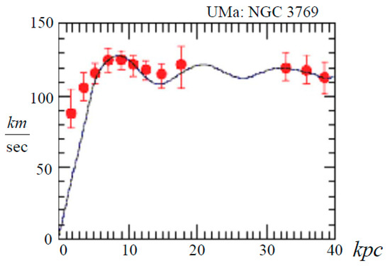
Figure 11.
Rotation curve of the spiral galaxy NGC 3769 in the Ursa Major cluster. The vertical axis is the speed in km/sec. The horizontal axis is the distance from the center of the galaxy in kiloparsecs. The solid line is fitting by Equation (67).
In References [3] and [10], the wavelength is considered as a unit of length. The argument of the covariant divergence is It follows from Equations (48)–(51) that on the horizon . Therefore, on the interface , the covariant divergence gets reduced to the usual one: When the scale is changed by q times, the ordinary derivative is transformed as Thus,
The balance of forces of gravitational attraction and centrifugal repulsion determines dependence of the velocity V(r) of a star, rotating around the center of a galaxy, on the radius. In a static spherical gravitational field, the centripetal acceleration is (Reference [6], problem 1 at the end of Section 88). Equality of centripetal acceleration to centrifugal V2/r gives
In the macroscopic theory of the dark sector [3], dark matter is described by the longitudinal vector field A black hole in the center is considered as a point-like object due to the small size of its radius when compared to the large size of a galaxy. The derivative dν/dr is expressed in terms of the covariant divergence of the field in the center (see Reference [3], Equation (86). This non-zero phenomenological parameter indicates the presence of a connection of dark matter with a black hole. Earlier, it was not possible to determine this connection without knowing what was going on inside a black hole. Now, the condition of phase equilibrium in Equation (55) at the interface between the longitudinal vector field (dark matter) and the gravitating scalar field (black hole) allows us to connect the covariant divergence of the longitudinal vector field to the parameters of a black hole. In particular, it allows us to express the velocity of rotation on the plateau as a function of the mass of a black hole.
Figure 9b,c show that, in the case of , the metric function g(x) (red curve) practically coincides with the Schwarzschild asymptote (dashed line) at . It means that, at the interface the gravitational field is weak. At , metric function The gravitational field is described by linearized Einstein equations,
Divergence of the longitudinal vector field obeys a linear Klein–Gordon equation,
In accordance with Equation (44),
The condition of phase equilibrium in Equation (55) at the interface between a scalar field and a longitudinal vector field determines the value . In the macroscopic theory [3], is a free parameter. In view of insignificance of the gravitational radius of a black hole in the scale of a galaxy ∼1022 cm, the value can be used as a boundary condition at The solution to Equations (61) and (62) is
Equations (8) and (63) determine the dependence of the dark matter wave function on the black hole mass: Local dark matter density is proportional to
Substituting Equation (63) into Equation (60), and using the identity,
we find
Substituting Equations (63) and (65) into Equation (59) and taking into account Equation (57), we get , which is needed for Equation (58).
In accordance with Equation (58), the dependence of the velocity V(r) of a circulating star on the distance r from the center of a galaxy is as follows:
where Vpl,
is the velocity on the plateau of a galaxy rotation curve. is the Plank mass. is the mass of a black hole, visible to a remote observer. m is the mass of a quantum of a scalar field, and μ is the mass of a quantum of a longitudinal vector field (dark matter). Equation (67) shows that the saturation of the function V(r) on the plateau is accompanied by damped oscillations [10].
Figure 11 shows the rotation curve of the spiral galaxy NGC 3769 of the Ursa Major cluster [3,10]. Dots with error bars are observations, copied from Reference [11]. The solid curve is the analytical dependence of the velocity on the radius (Equation (67)).
The plateau velocity of this galaxy is The period of damping oscillations is This corresponds to the de Broglie wavelength of a particle with a mass . On the basis of the standard model of elementary particles, the mass of a quantum of a scalar field with the rest energy about 100 GeV is . If the black hole at the center of the galaxy NGC 3769 in the Ursa Major cluster is really compressed to the state of condensation of scalar particles, then, according to Equation (68), its mass is three times larger than the solar mass:
7. Conclusions
Rejecting the prejudice that the signature of a metric tensor remains unchanged with an arbitrarily strong curvature of space-time, we get a possibility to clarify a number of long-standing questions. Considering a gravitating scalar field as an ordinary matter of a black hole, and a longitudinal vector field describing dark matter from outside, the possibility of a static equilibrium state of these two phases is shown. The main factor providing the ability to stop the collapse is the presence of a layer with a broken signature () inside the black hole. The corresponding static solutions of the Einstein equations do not require a limitation of the black hole mass. Super-massive black holes in the centers of galaxies, being in the state of phase equilibrium with the surrounding dark matter, form the skeleton of modern structure of the universe.
Funding
This research received no external funding.
Acknowledgments
I would like to thank Rachel Meierovich for editing this paper.
Conflicts of Interest
I declare no conflicts of interest.
References
- Gillessen, S.; Eisenhauer, F.; Trippe, S. Monitoring Stellar Orbits around the Massive Black Hole in the Galactic Center. Astrophys. J. 2009, 692, 1075. [Google Scholar] [CrossRef]
- Landau, L.D.; Lifshitz, E.M. Statistical Physics. Part 1; Nauka-Fizmatlit: Moscow, Russian, 1995. [Google Scholar]
- Meierovich, B.E. Macroscopic Theory of Dark Sector. J. Gravity 2014, 586958. [Google Scholar] [CrossRef]
- Landau, L.D.; Lifshitz, E.M. Statistical Physics. Part 2: Theory of the Condensed State; Fizmatlit: Moscow, Russian, 2002. [Google Scholar]
- Meierovich, B.E. On the Equilibrium State of a Gravitating Bose--Einstein Condensate. J. Exp. Theor. Phys. 2018, 127, 889–902. [Google Scholar] [CrossRef]
- Landau, L.D.; Lifshitz, E.M. The Classical Theory of Fields; Nauka: Moscow, Russian, 1973. [Google Scholar]
- Schwarzschild, K. Uber das Gravitationsfeld Eines Massenpunktes Nach Einsteinschen Theorie; Sitzungsberichte der Königlich Preußischen Akademie der Wissenschaften: Berlin, Germany, 1916; pp. 189–196. [Google Scholar]
- Colpi, M.; Shapiro, S.L.; Wasserman, I. Boson stars: Gravitational equilibria of self-interacting scalar fields. Phys. Rev. Lett. 1986, 57, 2485. [Google Scholar] [CrossRef] [PubMed]
- Andreev, A.F. Macroscopic bodies with zero rest mass. J. Exp.Theor. Phys. 1974, 38, 648. [Google Scholar]
- Meierovich, B.E. Galaxy rotation curves driven by massive vector fields: Key to the theory of the dark sector. Phys. Rev. D Part. Fields Gravit. Cosmol. 2013, 87, 103510. [Google Scholar] [CrossRef]
- Brownstein, J.R.; Moat, J.W. Galaxy rotation curves without non-baryonic dark matter. Astrophys. J. 2006, 636, 721. [Google Scholar] [CrossRef]
© 2019 by the author. Licensee MDPI, Basel, Switzerland. This article is an open access article distributed under the terms and conditions of the Creative Commons Attribution (CC BY) license (http://creativecommons.org/licenses/by/4.0/).