β⁻-Decay Half-Lives of Even-Even Nuclei Using the Recently Introduced Phase Space Recipe

Abstract

In this paper, we present the $\beta$-decay half-lives calculation for selected even-even nuclei that decay through electron emission. The kinematical portion of the half-life calculation was performed using a recently introduced technique for computation of phase space factors (PSFs). The dynamical portion of our calculation was performed within the proton-neutron quasiparticle random phase approximation (pn-QRPA) model. Six nuclei (${}^{20}$O, ${}^{24}$Ne, ${}^{34}$Si, ${}^{54}$Ti, ${}^{62}$Fe and ${}^{98}$Zr) were selected for the present calculation. We compare the calculated PSFs for these cases against the traditionally used recipe. In our new approach, the Dirac equation was numerically solved by employing a Coulomb potential. This potential was adopted from a more realistic proton distribution of the daughter nucleus. Thus, the finite size of the nucleus and the diffuse nuclear surface corrections are taken into account. Moreover, a screened Coulomb potential was constructed to account for the effect of atomic screening. The power series technique was used for the numerical solution. The calculated values of half-lives, employing the recently developed method for computation of PSFs, were in good agreement with the experimental data.

1. Introduction

In the last few decades, the $\beta$-decay process shaped our perspective of modern physics. From changing the evolution of the Standard Model and revealing the nature of left-handed ’$V-A$’ weak interaction [1], the theoretical study of $\beta$-decay also performed a key part in the understanding of astrophysical processes, such as nucleosynthesis ($r-$, $rp-$, $s-$, $p-$) processes and pre-supernova evolution of massive stars [2,3,4]. Probing different observables of $\beta$-decay continue to be at the forefront of new physics research, but dealing with the Hamiltonian that administers all types of $\beta$-decay is not a trivial problem and involves approximations.

The weak interaction which produces the real decay is much weaker as compared to the electromagnetic interaction of beta-particle with its neighborhood. Consequently, the later interaction may not be treated in the perturbation theory for nuclear $\beta$-decay Hamiltonian [5,6]. The typical approximation is to use the Dirac equation having an electrostatic potential instead of a plane-wave of $\beta$-particle [7]. With this replacement, the half-life for nuclear $\beta$-decay is calculated after the computation of associated nuclear matrix elements (NMEs) and PSFs.

In the literature, various approaches for $\beta$ spectrum description and PSF calculation were reported [8,9,10,11]. Some of these calculations employed the point charge Fermi function [12]. A realistic PSF must evaluate the $\beta$-particle radial wave function as solutions to the Dirac equation in a finite charge distribution that adequately describe that of the real nucleus [13]. In this paper, we used $\beta$-particle exact radial wave functions for the construction of the Fermi function acquired by solving the Dirac equation numerically with realistic electrostatic potential. In this approach, we included electrostatic finite-size corrections (finite size and diffuse nuclear surface) and atomic screening corrections by constructing an appropriate Coulomb potential. The numerical recipe used to solve the Dirac equation limited the truncation errors of solutions, and the only remaining discrepancies were because of rounding errors and distortion of potential initiated by the interpolating spline [14,15]. The present technique for the calculation of PSFs could easily be developed for any arbitrary nucleus. For further details about the new recipe of PSFs, we refer to [16].

Another consequence of the approximation discussed above is that the PSF calculation and $\beta$ spectrum predictions must include the electromagnetic correction. Examples for such correction are the emission of internal bremsstrahlung during decay and the interaction of the $\beta$-particle with the decaying nucleon. Hayen et al. [11] tabulated all corrections that should be applied on $\beta$ spectrum calculation. This type of correction is not included in the recently introduced recipe for calculation of PSF [16].

For the current half-lives calculation of $\beta$-decay, NMEs were calculated within the framework of the (pn-QRPA) model in a deformed basis and a schematic separable potential, both in particle-hole and particle-particle channels. In this work, we compute PSFs and ${\beta }^{-}$-decay half-lives for six even-even nuclei (${}^{20}$O, ${}^{24}$Ne, ${}^{34}$Si, ${}^{54}$Ti, ${}^{62}$Fe and ${}^{98}$Zr). We compare our PSFs [16] with the ones computed by Gove and Martin (GM) [17]. We later calculate the half-lives of $\beta$-decay for these selected nuclei using the traditional [17] and newly introduced [16] recipes for the computation of PSFs. The half-lives are further compared with the measured values.

We briefly describe the necessary formalism of reported work in Section 2. We discuss our results and compare them with measured data in Section 3. We report our findings in Section 4.

2. Theoretical Framework

The theoretical framework for computation of PSFs for any type of nuclear $\beta$ transition is presented in detail in Ref. [17]. We included only the allowed transitions (Fermi and Gamow-Teller type) in our calculations. The traditional PSF for an allowed $\beta$ transition is given in natural units ($\hslash =m=c=1$) by

$$f={\int }_1^{E_0}pE{(E_0-E)}^{2}F(Z,E)dE.$$

(1)

In “Equation (1)”, p denotes $\beta$-particle momentum, and E = $\sqrt{p^2+1}$ stands for total energy, while $E_0$ is the maximum energy of the $\beta$-particle. Many authors [10,18] start from the point charge Fermi function $F(Z,E)$;

$$F(Z,E)=4{\left(2pR\right)}^{2(\gamma -1)}{e}^{\pi \eta }\frac{{\left|\Gamma (\gamma +i\eta )\right|}^2}{{[\Gamma (2\gamma +1)]}^2}$$

(2)

introduced in 1934 [12]. In “Equation (2)”, $\alpha \simeq 1/137$ is the fine structure constant; $\gamma =\sqrt{1-{\alpha }^2{Z}^2}$; $\eta =\alpha ZE/p$; R is the radius of the nucleus in units of $\hslash /m_e{c}^2$; and $\Gamma$ is the gamma function. The Fermi function could be described in terms of the radial wave functions

$$F(Z,E,r)=\frac{f_1^2(Z,E,r)+g_{-1}^2(Z,E,r)}{2p^2},$$

(3)

which, historically, has been evaluated at the nuclear radius or the origin. In this paper, we consider the evaluation at the nuclear surface. The functions $f_1(Z,E,r)$ and $g_{-1}(Z,E,r)$ are small and large radial wave functions, respectively, and satisfy coupled equations [19],

$$\begin{array}{c}\hfill \begin{array}{ccc}\hfill \left(\frac{d}{dr}+\frac{\kappa +1}{r}\right)g_{\kappa }(E,r)& =& (E+V\left(r\right)+1)f_{\kappa }(E,r)\hfill \\ \hfill \left(\frac{d}{dr}+\frac{\kappa -1}{r}\right)f_{\kappa }(E,r)& =& -(E+V\left(r\right)-1)g_{\kappa }(E,r),\hfill \end{array}\end{array}$$

(4)

where $V\left(r\right)$ is the central potential of the $\beta$-particle, while $\kappa$ is the relativistic quantum number.

At this point, a comparison between our approach and the method presented by GM can be made. There are two major differences between the approaches. The GM recipe used the analytical radial wave function solutions of “Equation (4)” with $V\left(r\right)$ given by $-Z{e}^2/r$. The finite-size correction introduced by Rose and Holmes [20] has been later applied analytically to the obtained Fermi function. The advantage of numerically solving “Equation (4)” was that we introduced the finite-size correction and the diffused nuclear surface correction by choosing a proper electrostatic potential, presented below. The second difference between the two formalisms is the inclusion of the atomic screening correction. Whereas GM used the change of variables in the radial wave functions, we implemented this directly in the electrostatic potential.

The electrostatic potential used in this work was adopted from a more realistic proton density distribution in the nucleus, in comparison with a uniform one. The charge density was introduced using

$${\rho }_e\left(\overrightarrow{r}\right)=\sum _i(2j_i+1)v_i^2{\left|{\psi }_i\left(\overrightarrow{r}\right)\right|}^2,$$

(5)

where ${\psi }_i$ denotes the proton wave function for the spherical single-particle state i, and $v_i$ stands for the amplitude of occupation. By solving the Schrödinger equation using the Woods-Saxon potential, the wave functions ${\psi }_i$ were obtained. The (2$j_i$ + 1) term in “Equation (5)” reflects the degeneracy of spin. The difference between a uniform charge density and the one derived in this work can be found in “Figure 1”.

The Coulomb potential was obtained by integrating the realistic proton density distribution

$$V(Z,r)=\alpha \hslash c\int \frac{{\rho }_e(\overrightarrow{r^{\prime }})}{|\overrightarrow{r}-\overrightarrow{r^{\prime }}|}d\overrightarrow{r^{\prime }}.$$

(6)

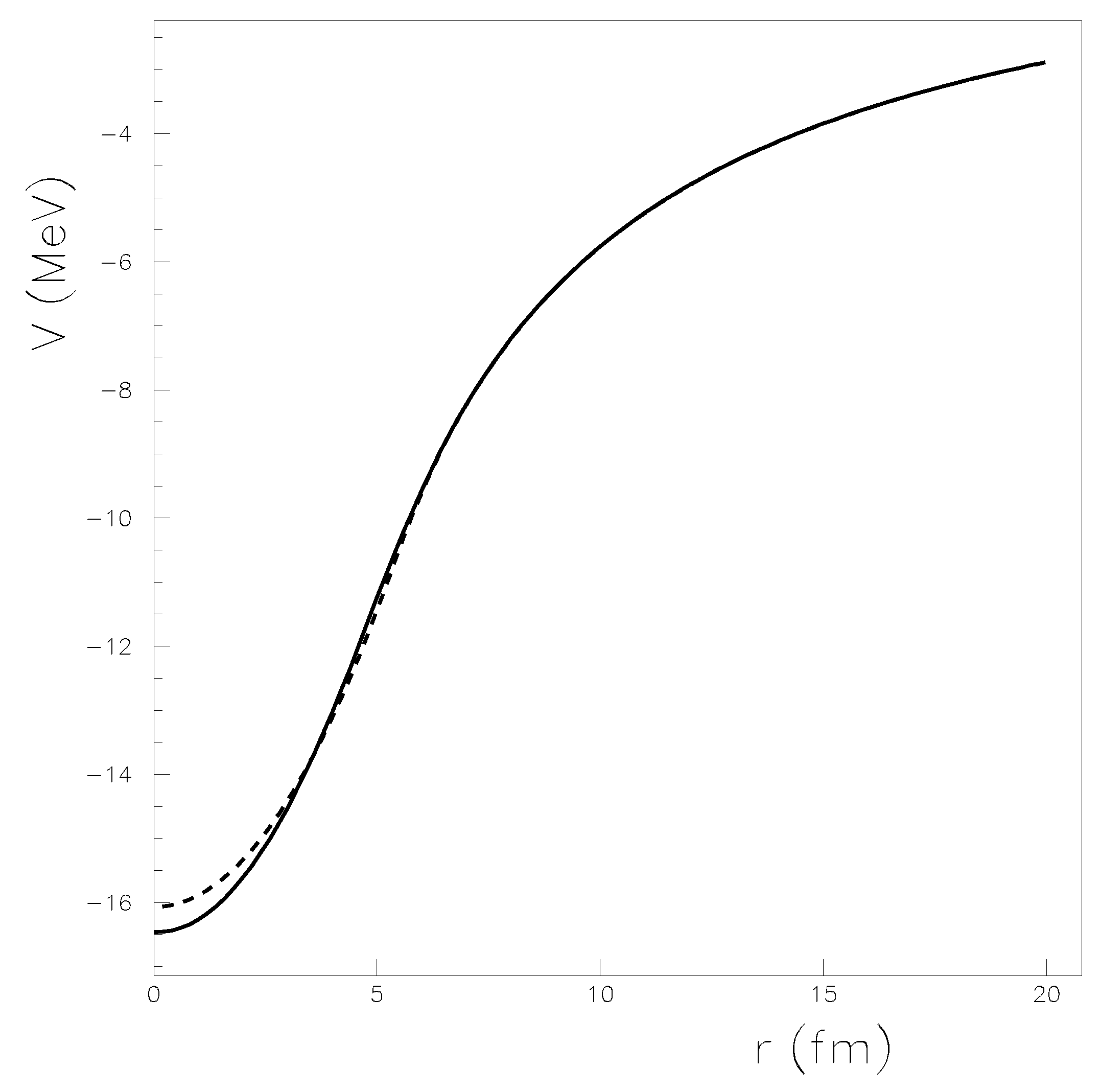
The Coulomb potential obtained with the “Equation (6)” is represented in “Figure 2” with a full curve for a residual nucleus with Z = 40 and A = 90. In the same figure, the Coulomb potential obtained with a constant charge density in the volume of the residual nucleus is also displayed with a dashed line. For some nuclei, the differences between the two potentials can lead to spreads which amount to 0.5% in the Fermi function. One considers that the potential obtained within the calculated proton density is more realistic.

Solutions of “Equation (4)” with the electrostatic potential described by “Equation (6)” include the finite-size and diffuse nuclear surface effects. Furthermore, we also consider the atomic screening effect by changing the expression of $V\left(r\right)$ with function $\varphi \left(r\right)$, that is, the solution for the Thomas-Fermi equation

$$\frac{d^2\varphi }{d{x}^2}=\frac{{\varphi }^{3/2}}{\sqrt{x}},$$

(7)

with $x=r/b$, where $b\approx 0.8853r_b{Z}^{-1/3}$ and $r_b$ is the Bohr radius. The solution $\varphi \left(r\right)$ was calculated using the Majorana recipe [21]. In the case of ${\beta }^{-}/{\beta }^{+}$, the effective potential $V_{{\beta }^{\mp }}$ was improved with the help of screening function $\varphi \left(r\right)$, as

$$r{V}_{{\beta }^{\mp }}(Z,r)=(rV(Z,r)+1)\times \varphi \left(r\right)-1.$$

(8)

$\beta$-decay half-lives were calculated by summing all transition probabilities to daughter excited states lying within the Q${}_{\beta }$ value

$$T_{1/2}={(\sum _{0\le E_x\le Q_{\beta }}1/t_x)}^{-1},$$

(9)

where t${}_x$ are the partial half-lives:

$$t_x=\frac{C}{{(g_A/g_v)}^2{F}_{A/V}B\left(E_x\right)}.$$

(10)

In “Equation (10)”, C is a constant whose value was taken as 6143 s [22], for the weak interaction $g_A$, $g_v$ denotes axial-vector and vector coupling constants, respectively, having $g_A$/$g_v$ = −1.2694 [23], while $E_x$ is the daughter excitation energy. $F_{A/V}$ are the PSFs discussed above. $B\left(E_x\right)$ are the reduced transition probabilities for the Fermi and Gamow–Teller (GT) transitions. We can express these reduced transition probabilities in the form of NMEs, as follows:

$$B_F\left(E_x\right)=\frac{1}{2I_i+1}\mid <x\Vert M_F\Vert i>{\mid }^2,$$

(11)

$$B_{GT}\left(E_x\right)=\frac{1}{2I_i+1}\mid <x\Vert M_{GT}\Vert i>{\mid }^2.$$

(12)

In “Equations (11) and (12)”, $I_i$ represents the spin of the parent state, and $M_F$ and $M_{GT}$ denote the Fermi and GT transition operators, respectively. A detailed description about the computation of NMEs using the pn-QRPA theory can be seen in Refs. [24,25].

We further explored the effect of pairing gaps on calculated PSFs and $\beta$-decay half-lives. The pairing gap computation proved crucial for the current calculation. For the calculation of the pairing gap, in units of MeV, we employed the so-called three-point formulae. These formulae are a function of neutron and proton separation energies, as shown in Equations (13) and (14)

$${\Delta }_{pp}=\frac{1}{4}{(-1)}^{Z+1}[S_p(A+1,Z+1)-2S_p(A,Z)+S_p(A-1,Z-1)]$$

(13)

$${\Delta }_{nn}=\frac{1}{4}{(-1)}^{A-Z+1}[S_n(A+1,Z)-2S_n(A,Z)+S_n(A-1,Z)].$$

(14)

For further details of the calculation of PSFs and NMEs, we refer to [16,26].

3. Results

Table 1. Calculated total phase space factors $F_{{\beta }^{-}}$ for ${\beta }^{-}$ decay, with Q-values from [27].

Nucleus	${\mathit{Q}}_{{\mathit{\beta }}^{-}}$ (MeV) [27]	${\mathit{F}}_{{\mathit{\beta }}^{-}}^{\left(\mathit{GM}\right)}$	${\mathit{F}}_{{\mathit{\beta }}^{-}}^{\left(\mathit{C}\right)}$
${}^{20}$O	3.81366	5864.37	5849.69
${}^{24}$Ne	2.46630	70.6367	70.4907
${}^{34}$Si	4.59170	5531.61	6167.34
${}^{54}$Ti	4.27300	26816.4	26556.5
${}^{62}$Fe	2.54600	2452.09	2422.20
${}^{98}$Zr	2.23800	3372.44	3294.33

shows the PSFs computed with the current and GM recipes for the six even–even selected nuclei. Q-values were taken from Ref. [27]. The two results differ at the maximum by 10 percent.

A comparison between the measured and calculated values of $\beta$-decay half-lives for the six selected nuclei are shown in

Table 2. Comparison of measured [27] and computed half-lives using PSFs by GM prescription of [17] and by newly introduced recipe (C) [16]. Half-life values are stated in units of s.

Nucleus	${\mathit{T}}_{1/2}^{\left(\mathit{EXP}\right)}$ (s) [27]	${\mathit{T}}_{1/2}^{\left(\mathit{GM}\right)}$ (s) [17]	${\mathit{T}}_{1/2}^{\left(\mathit{C}\right)}$ (s)
${}^{20}$O	(1.351±0.005) E+01	2.12E+01	1.49E+01
${}^{24}$Ne	(2.028±0.012) E+02	2.26E+02	2.05E+02
${}^{34}$Si	(2.770±0.200) E+00	3.01E+00	2.87E+00
${}^{54}$Ti	(2.100±1.000) E+00	3.14E+00	2.41E+00
${}^{62}$Fe	(6.800±0.200) E+01	9.24E+01	7.68E+01
${}^{98}$Zr	(3.070±0.040) E+01	4.06E+01	3.33E+01

. Measured half-lives appearing in the second column were taken from [27]. Computed half-lives in the third column were obtained using the traditional PSF recipe of GM and associated NMEs from the pn-QRPA model. The last column presents the calculated half-lives employing the newly introduced PSFs and labeled $\left(C\right)$ (current). The associated NMEs were calculated within the framework of the pn-QRPA model. Half-life values in Table 2 are stated in units of seconds. One notes that the GM half-life values are systematically bigger than those calculated using the current recipe. It is noted that the calculated half-lives using the new prescription of PSFs are in better agreement with the experimental data. This is an important finding of the current work.

Table 3. State-by-state comparison of computed $\beta$-decay half-lives using the GM and newly introduced recipes for computation of PSFs. The daughter energy levels, NMEs, Q values, partial half-lives t${}_f$ and branching ratio I${}_{\left({\beta }^{-}\right)}$ for ${\beta }^{-}$-decay to calculated daughter states are also shown.

${}^{20}$O
E${}_{\mathit{x}}$ (MeV)	NME	${\mathit{Q}}_{{\mathit{\beta }}^{-}}$(MeV)	${\mathit{F}}_{{\mathit{\beta }}^{-}}^{\left(\mathit{GM}\right)}$[17]	${\mathit{F}}_{{\mathit{\beta }}^{-}}^{\left(\mathit{C}\right)}$	t${}_{\mathit{f}}^{\left(\mathit{GM}\right)}$[17]	t${}_{\mathit{f}}^{\left(\mathit{C}\right)}$	I${}_{\left({\mathit{\beta }}^{-}\right)}^{\left(\mathit{GM}\right)}$[17]	I${}_{\left({\mathit{\beta }}^{-}\right)}^{\left(\mathit{C}\right)}$
0.00400	0.00000	3.80967	1689.06	1684.56	1.40644E+06	4.87374E+05	0.0020	0.0030
0.24900	0.01929	3.56411	1252.16	1249.04	1.65717E+02	4.16003E+01	12.810	17.260
0.26200	0.03908	3.55175	1232.83	1229.70	8.30920E+01	4.80330E+01	25.549	35.898
0.54200	0.09132	3.27209	854.878	852.899	5.12796E+01	9.48294E+01	41.399	31.091
0.55800	0.04569	3.25521	835.436	833.484	1.04884E+02	6.66259E+03	20.240	15.748
${}^{34}$Si
0.70800	0.26574	3.88335	2167.55	2414.32	6.94985E+00	6.65015E+00	43.421	43.163
0.84300	0.00000	3.74878	1850.47	2062.28	1.54665E+08	1.60074E+08	0.0000	0.0000
1.07200	0.53771	3.51923	1395.43	1557.01	5.33510E+00	5.05171E+00	56.563	56.821
2.66400	0.00000	1.92758	102.739	115.983	2.09311E+09	1.19578E+09	0.0000	0.0000
3.47600	0.01324	1.11531	11.0202	12.6278	2.74395E+04	2.64834E+04	0.0110	0.0110
3.82500	0.00000	0.76635	2.57740	2.99066	4.10905E+11	3.83127E+11	0.0000	0.0000
3.96800	0.05621	0.62359	1.19018	1.39208	5.98407E+04	5.67186E+04	0.0050	0.0050
4.06900	0.00000	0.52264	0.62227	0.73302	3.54261E+12	3.28252E+12	0.0000	0.0000

presents the state-by-state computation of partial half-lives for ${}^{20}$O (the largest difference between the two calculations as noted in Table 2) and ${}^{34}$Si (the smallest difference between the two calculations). The values of the pn-QRPA model calculated daughter excitation energies ($E_x$), $Q_{{\beta }^{-}}$ (= $m_p-m_d-E_x$), PSFs, NMEs, and branching ratios I${}_{\left({\beta }^{-}\right)}$ are also given in Table 3. For the case of ${}^{20}$O, we note that the partial half-lives and branching ratios to the last four levels contribute to the big difference between the two calculations. The computed branching ratios and partial half-lives are in decent agreement for all states in the case of ${}^{34}$Si.

4. Conclusions

In this paper, the newly introduced prescription of PSFs were applied to compute $\beta$-decay half-lives of even–even nuclei. The required NMEs were computed within the framework of the pn-QRPA model. A small difference between the traditionally and newly introduced recipe of PSFs was noted. A similar difference was also reported for the computed values of $\beta$-decay half-lives using the two recipes of PSFs. The newly introduced recipe of PSFs resulted in calculated $\beta$-decay half-lives that was in better agreement with the measured ones. In the future, we plan to expand our study of beta-decay half-life values to a large pool of nuclei undergoing ${\beta }^{-}$, ${\beta }^{+}$, and electron capture decays. We also plan to study the effect of introducing the new recipe of PSFs on double-beta decay half-lives and beta decays in a stellar environment.

References

- Weinberg, S. V-A was The Key. J. Phys. Conf. Ser. 2009, 196, 012002. [Google Scholar] [CrossRef] [Green Version]
- Möller, P.; Pfeiffer, B.; Kratz, K.L. New calculations of gross β-decay properties for astrophysical applications: Speeding-up the classical r process. Phys. Rev. C 2003, 67, 055802. [Google Scholar] [CrossRef] [Green Version]
- Ni, D.; Ren, Z. β-decay rates of r-process waiting-point nuclei in the extended quasiparticle random-phase approximation. J. Phys. G Nucl. Part. Phys. 2014, 41, 025107. [Google Scholar] [CrossRef]
- Ren, Y.; Ren, Z. Systematic law for half-lives of double-β decay with two neutrinos. Phys. Rev. C 2014, 89, 064603. [Google Scholar] [CrossRef] [Green Version]
- Groote, H.V.; Hilf, E.R.; Takahashi, K. A new semiempirical shell correction to the droplet model: Gross theory of nuclear magics. At. Data Nucl. Data Tables 1976, 17, 418–427. [Google Scholar] [CrossRef]
- Halpern, T.A. Static Coulomb Correction to Beta Decay Arising from the Nuclear Charge Change: A Nonperturbative Approach. Phys. Rev. C 1970, 1, 1928–1938. [Google Scholar] [CrossRef]
- Roman, P. Advanced Quantum Theory; Addison-Wesley Publishing Company, Inc.: Reading, MA, USA, 1965. [Google Scholar]
- Behrens, H.; Bühring, W. ft values of superallowed 0-0 transitions. Nucl. Phys. A 1968, 106, 433. [Google Scholar] [CrossRef]
- Behrens, H.; Bühring, W. On the sensitivity of β-transitions to the shape of the nuclear charge distribution. Nucl. Phys. A 1970, 150, 481–496. [Google Scholar] [CrossRef]
- Konopinski, E.J.; Uhlenbeck, G.E. On the Fermi Theory of β-Radioactivity. II. The “Forbidden” Spectra. Nucl. Phys. Rev. 1941, 60, 308. [Google Scholar] [CrossRef]
- Hayen, L.; Severijns, N.; Bodek, K.; Rozpedzik, D.; Mougeot, X. High precision analytical description of the allowed β spectrum shape. Rev. Mod. Phys. 2018, 90, 015008. [Google Scholar] [CrossRef] [Green Version]
- Fermi, E. Versuch einer Theorie der β-Strahlen. I. Zeitschrift fur Phys. 1934, 88, 161–177. [Google Scholar] [CrossRef]
- Wilkinson, D.H. Evaluation of β-decay: II. Finite mass and size effects. Instruments Methods Phys. Res. A 1990, 290, 509–515. [Google Scholar] [CrossRef]
- Salvat, F.; Mayol, R. Accurate numerical solution of the Schrödinger and Dirac wave equations for central fields. Comp. Phys. Commun. 1991, 62, 65–79. [Google Scholar] [CrossRef]
- Salvat, F.; Fernandez-Varea, J.M.; Williamson, W., Jr. Accurate numerical solution of the radial Schrödinger and Dirac wave equations. Comp. Phys. Commun. 1995, 90, 151–168. [Google Scholar] [CrossRef]
- Stoica, S.; Mirea, M.; Niţescu, O.; Nabi, J.; Ishfaq, M. New Phase Space Calculations for β-Decay Half-Lives. Adv. High Energy Phys. 2016, 2016, 8729893. [Google Scholar] [CrossRef] [Green Version]
- Gove, N.B.; Martin, M.J. Log-f tables for beta decay. Nucl. Data. Tables 1971, 10, 205–219. [Google Scholar] [CrossRef]
- Behrens, H.; Jänecke, J. Numerical Tables for Beta-Decay and Electron Capture; Springer: Berlin/Heidelberg, Germany, 1969. [Google Scholar]
- Rose, M.E. Relativistic Electron Theory. Phys. Today 1961, 14, 58. [Google Scholar] [CrossRef]
- Rose, M.E.; Holmes, D.K. Oak Ridge National Laboratory Report ORNL-1022. Phys. Rev. 1951, 83, 190. [Google Scholar] [CrossRef]
- Esposito, S. Majorana solution of the Thomas-Fermi equation. Am. J. Phys. 2002, 70, 852–856. [Google Scholar] [CrossRef] [Green Version]
- Hardy, J.C.; Towner, I.S. Superallowed 0+ 0+ nuclear β decays: A new survey with precision tests of the conserved vector current hypothesis and the standard model. Phys. Rev. C 2009, 79, 055502. [Google Scholar] [CrossRef] [Green Version]
- Nakamura, K. Review of particle physics. J. Phys. G Nucl. Part. Phys. 2010, 37, 075021. [Google Scholar] [CrossRef] [Green Version]
- Hirsch, M.; Staudt, A.; Muto, K.; Klapdorkleingrothaus, H.V. Microscopic Predictions of β+/EC-Decay Half-Lives. At. Data and Nucl. Data Tables 1993, 53, 165–193. [Google Scholar] [CrossRef]
- Staudt, A.; Bender, E.; Muto, K.; Klapdor- Kleingrothaus, H.V. Second generation microscopic predictions of beta decay half-lives of neutron rich nuclei. At. Data. Nucl. Data. Tables 1990, 44, 79–132. [Google Scholar] [CrossRef]
- Ishfaq, M.; Nabi, J.-U.; Niţescu, O.; Mirea, M.; Stoica, S. Study of the Effect of Newly Calculated Phase Space Factor on β-Decay Half-Lives. Adv. High Energy Phys. 2019, 2019, 5783618. [Google Scholar] [CrossRef]
- Audi, G.; Kondev, F.G.; Wang, M.; Huang, W.J.; Naimi, S. The NUBASE2016 evaluation of nuclear properties. Chin. Phys. C 2017, 41, 030001. [Google Scholar] [CrossRef]
Figure 1.
(a) Realistic proton density for an atomic number Z = 40 represented in cylindrical coordinates; (b) Profile of the realistic proton density for Z = 40 (thick line) compared with that given by a constant density approximation (dot-dashed line).
Figure 2.
Comparison between the Coulomb potential obtained with a realistic charge density displayed with a full line, and a potential obtained within a constant charge density plotted with a dashed line for a Z = 40 residual nucleus.