
Sparsity and M-Estimators in RFI Mitigation for Typical Radio Astrophysical Signals
by
 , , , ,
Hao Shan
1,2,*,
Ming Jiang
3,*,
Jianping Yuan
1,2,
Xiaofeng Yang
1,2,
Wenming Yan
1,2,
Zhen Wang
1,2 and
Na Wang
1,2 1
Xinjiang Astronomical Observatory, Chinese Academy of Sciences, No. 150, Science Street 1st, Urumqi 830011, China
2
Xinjiang Key Laboratory of Radio Astrophysics, No. 150, Science Street 1st, Urumqi 830011, China
3
National Key Laboratory of Radar Signal Processing, Xidian University, No. 2, South Taibai Road, Xi’an 710071, China
*
Authors to whom correspondence should be addressed.
Universe 2023, 9(12), 488; https://doi.org/10.3390/universe9120488
Submission received: 14 August 2023
/
Revised: 8 November 2023
/
Accepted: 10 November 2023
/
Published: 23 November 2023
(This article belongs to the Special Issue A New Horizon of Pulsar and Neutron Star: The 55-Year Anniversary)
Abstract
:In this paper, radio frequency interference (RFI) mitigation by robust maximum likelihood estimators (M-estimators) for typical radio astrophysical signals of, e.g., pulsars and fast radio bursts (FRBs), will be investigated. The current status reveals several defects in signal modeling, manual factors, and a limited range of RFI morphologies. The goal is to avoid these defects while realizing RFI mitigation with an attempt at feature detection for FRB signals. The motivation behind this paper is to combine the essential signal sparsity with the M-estimators, which are pertinent to the RFI outliers. Thus, the sparsity of the signals is fully explored. Consequently, typical isotropic and anisotropic features of multichannel radio signals are accurately approximated by sparse transforms. The RFI mitigation problem is thus modeled as a sparsity-promoting robust nonlinear estimator. This general model can reduce manual factors and is expected to be effective in mitigating most types of RFI, thus alleviating the defects. Comparative studies are carried out among three classes of M-estimators combined with several sparse transforms. Numerical experiments focus on real radio signals of several pulsars and FRB 121102. There are two discoveries in the high-frequency components of FRB 121102-11A. First, highly varying narrow-band isotropic flux regions of superradiance are discovered. Second, emission centers revealed by the isotropic features can be completely separated in the time axis. The results have demonstrated that the M-estimator-based sparse optimization frameworks show competitive results and have potential application prospects.
1. Introduction
RFI originating from a variety of human-produced sources becomes one of the main challenges in radio observation [1]. These sources are mainly made by human communication technologies, e.g., satellites, mobile base stations, navigation radars, cell phones, televisions, and air traffic communications. Different types of RFI display different amplitudes and time–frequency distributions. Frequently, several types of RFI can appear as a mixed form in groups of narrow and broad bands [1]. Channel saturation in some perhaps successive channels caused by the transiently strong RFI is one of the most severe cases of signal loss because no useful information can be identified in these channels. Thus, the channel mask by some centrality measures (e.g., local median) is often applied for narrow-band transiently strong RFI. The complexity of its overall distribution makes it difficult to give a general model for the mitigation problem [2].
There are several categories in the discipline of RFI mitigation. The linear mitigation methods form the first category, including, for example, the principal component analysis (PCA) [3] and singular vector decomposition (SVD) [4,5]. Several typical examples from the category of thresholding methods are the cumulative sum (CUSUM) [6], VarThreshold, and SumThreshold [1]. Other examples include a spectral kurtosis-based thresholding method [7,8], a zero-DM filtering [9], and a pulsar phase and standard deviation (PPSD) [10].
Over the last decade, a new category, including transform domain thresholding methods, has gained extensive applications. In contrast to the second category, these methods usually threshold the transform domain coefficients. Sparse transforms play the role of protagonists in this category. Maslakovic et al. (1996) [11] proposed to excise RFI based on optimizing the entropy of discrete wavelet transform. Based on the wavelet transform, Demorest et al. (2013) [12] introduced a plugin function into the toolbox of . Both recent works [13,14] were based on sparse representation and optimization. Shan et al. (2022) [13] focused on pulsar signal restoration by the idea of compressed sensing for the masked channels in preprocessing. The work by Shan (2023) [14] was based on a LnCosh filter, one of the M-estimators, to explore the nonlinear robust property. Both [14] and this paper apply the M-estimators; however, this paper further extends the work of [14] by various kinds of M-estimators and to feature representation for FRB signals.
The category of nonlinear methods can be classified into two branches. The first branch is based on ML and neural networks (NNs), and the other one applies nonlinear filters. Several examples of the first branch are as follows. Vos et al. (2019) [15] presented an unsupervised ML approach by applying a generative adversarial network (GAN) to separate the spectrogram into components of signal and RFI. Applications of deep neural networks [16] and convolutional neural networks (CNNs) [17] start to prosper, e.g., a U-Net (one type of CNN)-based RFI mitigation [18], and a robust CNN model for RFI identification [19]. However, the learning and training processes of some ML techniques, especially the traditional ones, are time-consuming and computationally expensive. The second branch of nonlinear filtering is still marginal within subfields of time-domain astronomy. In this branch, Hogden et al. (2012) [20] found that the Huber filter [21] is effective at removing the broad-band RFI. However, research work related to this idea has not been promoted. The framework proposed in this paper can be considered to be an improved technique of the second branch by combining fast optimization algorithms with sparse transforms.
For the task of RFI mitigation, two core factors need to be attentively considered. First, the non-Gaussian nature of RFI is one root cause of the current defects. Second, optimal approximation in such a case is a challenging task due to the vulnerability of radio signals versus huge amplitudes and complex distributions of RFI. A pertinent scheme specially targeted on the outlier attribute of RFI is necessary. In the scheme of this paper, the M-estimators, which form one of the most important branches in the category of robust estimators, will be introduced into RFI mitigation, and optimal approximation for signals containing the astrophysical features will be accomplished by signal sparsity.
Signal features are essential in parameter identification of radio sources and limitation setting on intrinsic physical emission mechanisms. Considering the time–frequency distributions of radio flux, typical signal features can be classified into isotropic (or quasi-isotropic) features [22,23] and anisotropic ones [24]. The isotropic ones of high-energy radio sources usually appear in the form of narrow-band flux (without consideration of frequency mask of some narrow bands), e.g., isotropic flux regions of the downward frequency drifting of FRBs, i.e., the narrow-band processes emitted at multiple descending frequencies. The task of this paper is to detect the isotropic narrow-band processes not only in low frequencies but also in high frequencies. The anisotropic features are reflected in, e.g., the curve-like dispersion relationship of pulsar signals and the elongated flux extensions of FRB signals in the time–frequency domain. For FRB signals at high frequencies, the anisotropic features are elliptical, and signals at low frequencies are roughly curve-like. In our opinion, these two classes of features have a common essence of sparsity in transform domains. Thus, sparse representation (e.g., wavelets [25,26,27,28,29]) can be applied to accomplish the tasks of feature approximation and detection.
This paper tries to build a robust nonlinear estimation framework covering different classes of M-estimators by exploring the essential sparsity of the astrophysical features with wavelets and geometric wavelets. Thus, the work in [14] is extended. An assumption is that signals from, e.g., pulsars and FRBs, are sparse in transform domains. The motivation is to combine the sparsity with the nonlinear robust property of the M-estimators. The goal is to avoid the current defects when we mitigate RFI in pulsar and FRB signals. This paper is organized as follows. The M-estimators are reviewed in Section 2. Section 3 gives several astrophysical features and interprets the sparse representation. Section 4 shows the mitigation model. Experimental results are given in Section 5. Finally, the conclusions are drawn in Section 6.
2. A Review of the M-Estimators
The three main branches of the robust estimators are formed by the L-estimators, R-estimators, and M-estimators. The L-estimators are defined as linear combinations of order statistics of the observations, resulting in their simple expressions (e.g., the sample median and trimmed mean (-trimmed mean) [30,31]) and robust statistics. The R-estimators are based on waste ranking and involve parameter estimation based on ranks of residuals [32,33]. The R-estimators classify a sample by a mapping of n real numbers and are resistant to outliers. Compared with the M-estimators, the L- and R-estimators belong to nonparametric statistical approaches and are convenient in calculation. However, definitions of the robust properties of the L- and R-estimators are difficult to obtain a priori [31]. On the contrary, this problem does not exist with the M-estimators. The shapes of the M-estimators are defined by fixed functions [31], which are simpler to handle. Thus, they are preferred, although they are sometimes computationally expensive. The robustness of the M-estimators lies in the fact that they are less sensitive to outlier deviations due to their intrinsic mathematical structures. One of the most typical estimators in the branch of the M-estimators is the Huber estimator, which has interpreted the generalization of the M-estimators. Huber (1973) [34] extended the idea of the M-estimators in solving the regression problem through minimizing a function of residuals, and this function has some popular properties, e.g., continuous and symmetrical, strictly positive and integrable, increasing monotonous, smooth and preferentially convex.
Suppose , denote a population of measurements following a probability function , are the estimated variables, and errors represent the random white Gaussian noise (WGN). The maximum likelihood formulation assumes that are uncorrelated so that the measurements are independent and the respective covariance matrices containing the variance values of the measurements are diagonal. Thus, the joint probability function p can be represented as a product of the individual probability functions , i.e.,
To facilitate calculation, a logarithm operator is applied such that
Generally, the M-estimators can be built from Equation (2). For example, the weighted least square (WLS) estimator (or estimator; [35]) is derived from the normal distribution
where denote the standardized residuals weighted by the standard deviations . Another example is the Cauchy estimator, which is built based on the Cauchy distribution
A generalization of the maximum likelihood objective function was first proposed by Huber (1964) [21]. Then, the idea of M-estimators was extended by Huber (1973) [34] in solving the regression problems by defining
which minimizes a smooth, symmetrical and monotonic [33] function of residuals, where and denote the mean value and standard deviation of the i-th variable in the sample set. One can estimate with the help of some iterative procedures [36]. The influence function [37] is a qualitative measure of robustness [38,39], and is defined as , which is the first partial derivative of the objective function with respect to the standardized residual . According to the descending behaviors of the influence functions, de Menezes et al. (2021) [33] summarized the classification of the M-estimators in detail. The non-robust M-estimators, e.g., the WLS estimator, have an unlimited influence function . The quasi-robust M-estimators (see Page 101 of [35]) refer to the ones that are more robust than the WLS estimator but without strict robustness. This paper will not cover these two classes of estimators.
Another class includes three kinds of robust M-estimators. The robust monotone M-estimators have convex influence functions, and typical examples are the Huber [21] and Zhang [40] estimators. Robust ones with decreasing influence functions are classified as redescending ones. According to Holland and Welsch (1977) [41], the redescending estimators can be further classified as soft-redescending (or pseudo-convex; e.g., the Cauchy and Welsch estimators [35]) and hard-redescending (or quasi-convex; e.g., the Biweight [35], Andrews [42], and Smith [43] estimators) ones depending on whether a certain influence function is approximately null or exactly null for high outlier values. Table 1 lists seven M-estimators belonging to the three kinds, and they will be applied in this paper.
3. Sparse Representation and Features of Radio Signals
3.1. Sparse Representation
Assume that has the property of “sparsity”, i.e., is N-sparse in a basis or a frame , such that can be expressed by N non-zero coefficients in , i.e., , where denote the coefficients under the sparse transform . In most cases, natural signals are not strictly sparse. Thus, the assumption of “sparsity” can be relaxed to “compressibility” if most of the energy in is contained in its largest N coefficients. Wavelets have been successfully applied to the detection of isotropic features. For example, the isotropic undecimated wavelet transform (IUWT) or starlet [22] has gained remarkable successes in galaxy images and has been proven to be well adapted to typical isotropic astronomical features in most cases [23]. Although two-dimensional (2D) wavelets can also be applied to the detection of curve-like features [44,45], being tensor products and separable extensions of 1D wavelet bases, they have a limited capability in isolating the directional information presented in natural signals. By contrast, shearlet [46,47] is specially designed to capture directional information of anisotropic features efficiently. Let be the N-term shearlet approximation of , shearlet is theoretically optimal in representing piecewise smooth objects with the second-order continuously differentiable singularities (i.e., C-singularities) by an asymptotic approximation error , , which is close to the optimal rate . However, the approximation error for a wavelet representation decays by as N increases. Although curvelet [48,49] also allows an optimal sparse representation for C curves and is the only other system known to satisfy similar approximation properties, it cannot form an affine system as the shearlet does. This is because curvelet is not obtained by applying dilations and translations to a single generating (or mother) function [50], and the angle in its triple indexes is defined in polar coordinates. What motivates us are the above representation and approximation abilities of the sparse transforms well suited to specific radio features. Appendix A gives a short review for the construction of the shearlet. For detailed theories and applications of the wavelets and curvelet, one can refer to [22,23] and [48,49,50], respectively. Figure 1 takes the dispersion relationship of a simulated pulsar signal as an example and gives a diagram to interpret the principles of sparse representation. The upper and lower halves of the signal are represented by the wavelet and shearlet, respectively. The squares and ellipses denote the spatial supports of wavelet and shearlet bases fitting the signal on different scales (from coarser to finer scales, the red, orange, and blue colors are used, respectively), where j is a scale, and are the lengths of the long and short axes of the spatial supports, respectively.
3.2. Examples of Astrophysical Features
The distributions of radio flux can be measured in different directions. If the distribution properties of a feature in all directions are the same, it indicates that the feature is independent of direction and is called isotropic. If the properties and directions are closely related, i.e., the properties of different directions are significantly different, one obtains an anisotropic feature. This subsection discusses several isotropic and anisotropic astrophysical features in multichannel time–frequency radio signals. These features not only directly reveal the basic properties and propagation effects but also are typically tailored for sparse transforms.
- Dispersion relationship. Search processes for radio astrophysical sources in multichannel signals consist of looking for dispersed pulses. In observed signal profiles, different observing frequency channels correspond to different amounts of dispersions. The dispersion frequency relationship [51,52] at (which is the central frequency of channel a) is calculated aswhere () is the dispersion constant, and is the reference frequency, which is chosen to be the center frequency of the broad band (with and as the central frequencies of the lowest and highest channels). The dispersion measure is defined as , where is the electron number density, l is the path length along the line-of-sight, and d is the distance to a radio source. This dispersion relationship is a widely presented feature in multichannel radio signals. The dispersion effect generates curve-like signals with typical C singularities. In this paper, the shearlet will be first applied in RFI mitigation of pulsar signals, and it is expected to guarantee accurate sparse representation and approximation for this feature.
- In FRB signals, the isotropic narrow-band superradiance, and directional time–frequency extensions (including extensions around the downward frequency drifting; distortions by the scattering effect). The dispersion effect will not be considered for the dedispersed FRB signals applied in this paper. Around the isotropic flux areas of superradiance, there are curve-like and local elliptical time–frequency extensions. Accurate approximation for these extensions helps to explore the changing trend of energy envelope and energy distribution morphologies.Subbursts in FRB signals have characteristic frequencies that drift lower at later times in the total burst envelope. FRB spectra with downward frequency drifting differ from those smooth and wide-band spectra of typical pulsars and radio-emitting magnetars. The dynamical and relativistic model proposed by Rajabi et al. (2020) [53] can explain the downward frequency drifting in multicomponent bursts according to Dicke’s superradiance. According to [53], superradiance occurs in a medium moving at relativistic speeds. This will cause narrow-band processes to be emitted at multiple descending frequencies in FRBs. In this paper, the narrow-band flux regions are regarded as isotropic (or quasi-isotropic) features and will be characterized by wavelets. The anisotropic drifting extensions with diffusing energy will be represented by curvelet.The scattering effect can temporally broaden the FRB signals and induce multi-path propagation, resulting in later arrival times for the signal portions traveling longer path [52]. Scattering tails can be seen in a large proportion of FRB signal profiles. Aggarwal et al. (2021) [54] modeled the components of the FRB spectra as the convolution of a Gaussian function (with a median width of 230 MHz) with a one-sided exponential function. The scattering measure (SM) defines the distribution of free electrons along the line-of-sight, where indicates the strength of the fluctuations along the line-of-sight. The scattering effect reflected in the profiles complicates the signal shapes, but it can be fitted along with the signal portions by the highly directionally sensitive needle-shaped base functions of curvelet on different scales.
4. Mitigation Model for Multichannel Radio Signals
Suppose that an observed multichannel signal profile consists of the radio signal of interest , the RFI , and the random GWN , i.e., . To avoid the susceptibility of the LS estimator to the presence of RFI outliers [55], a robust M-estimator with a nonnegative penalty function can be directly applied
where denotes the approximation of . Assume that the multichannel radio signals are sparse in transform domains, a sparsity-promoting -norm is well suited to assist the reconstruction. The first term aims to ensure that the approximated signal is close to the observed one in the sense of robust estimation, and the second term is to guarantee that is sparse under the sparse analysis of . Thus, is a regularization parameter determining the tradeoff between data fidelity and sparsity. To solve the nonlinear problem in Equation (7) with a sparsity-promoting term, a linearization process should be supplemented. Thus, the theory of pseudo-data [56] is applied, then one obtains , where is the pseudo-data of . Then, the problem can be solved by an algorithm of, e.g., the gradient projection [57,58], Newton [59], ISTA, or FISTA [60]. In this paper, the FISTA algorithm is taken as an example
where k is the step of iteration, is a decreasing update factor. If the maximum iteration step of FISTA is , then . Due to the huge difference between signal portions and RFI (especially for pulsar signals), the standard deviation can be directly calculated from the original time–frequency domain over the pseudo-data, i.e., , and . The threshold is calculated by , where q is a parameter that can be adjusted, and and are the sparse transform and its inverse transform. is a 2D mask in the preprocessing. Its entries are zeros on the positions of the zero set channels and ones on the others. For details about the preprocessing strategy, one can refer to [14].
In the tests of pulsar signals, a shearlet is used to realize the optimal representation and approximation. In the tests of FRB signals, the wavelets and curvelets are applied. The thresholds of shearlet and curvelet are calculated according to their default settings with as inputs. The threshold of the wavelet is calculated as without the decreasing update factor. In most cases of this paper, the q for wavelet is set to 3. According to the framework (7), an evaluation indicator termed signal to interference and noise ratio (SINR; in dB) is applied, and it is defined as , where . Please note that this definition is based on the theory of pseudo-data.
5. Experimental Results
5.1. Pulsar Signals
In the tests of pulsar signals, observations were made with the Nanshan 26-m Radio Telescope, which has a dual-channel cryogenic receiver with a reference frequency (or center frequency) of = 1556 MHz. For practical observations, a broad band from 1300.5 to 1812 MHz with a total bandwidth of 512 MHz is applied. The digital filter bank is configured to MHz channels and 8-bit sampling. Signal profiles of PSRs J1645−0317 (Figure 2), J1136+1551 (Figure 3), J0814+7429 (Figure 4), and J0332+5434 (Figure 5) are selected. They are folded data with 30 seconds integrated into one phase. All M-estimators applied in this test have already been shown in Table 1. Tuning parameters of the estimators are specified by their default values in Table 1. Unless otherwise specified, the following tests of FRB signals with wavelets and curvelet will always use this parameter setting. For pulsar signals with shearlet, the values of parameter q have been examined in repeated experiments for better SINR values. For J0332+5434, the Zhang estimator uses and the others use . For other pulsar signals, the Huber one uses , and the other estimators apply . Empirically, the selected q of the methods make them work well. Generally speaking, the higher the q, the more RFI is removed. However, higher q will also lead to oversmoothed or excessively attenuated mitigation results, and valuable details for astrophysical purposes will be lost.
In the mitigation process, the preprocessing can only obtain just-visible signals to naked eyes. From Figure 2, Figure 3, Figure 4 and Figure 5, by visual inspection, one can see that most types of RFI can be successfully removed, especially the narrow-band transient and quasiperiodic RFI. Actually, when the mitigation is proceeding with a fixed threshold, most types of RFI are removed gradually. Significantly, the types of quasiperiodic and long-period RFI are too obstinate to eliminate.
Generally speaking, by visual inspection of the four figures, one can see that among the M-estimators, the monotone ones (Huber and Zhang) show the best results, and the soft-redescending ones (Cauchy and Welsch) perform at a middle level. In the soft-redescending estimators, the Cauchy one has a performance close to those of the monotone ones, and the Welsch estimator performs similarly to the hard-redescending ones, which give relatively poor performances. Table 2 shows that the Huber estimator has the strongest robustness to RFI, and the trend reflected by the SINR values is consistent with that of the visual inspection. The Cauchy estimator performs well for pulsar signals with wider relative pulse widths in one phase (e.g., it has the best SINR values for PSRs J1136+1551 and J0814+7429). The proposed frameworks overcome the current defects in an obvious fact that most types of RFI have been removed for almost all the M-estimators in the applied pulsar signals.
Figure 6 shows dedispersed pulses by the seven estimators for the processed profiles of J0332+5434. A randomly selected band containing 50 consecutive channels is dedispersed, and the channels are added up. The iteration numbers are also shown in each panel. By visual inspection throughout the panels, the monotone estimators, i.e., Huber and Zhang estimators, perform the best.
5.2. FRBs
FRBs, especially the repeating ones [61,62] show complex and varying time–frequency structures, e.g., multiple-burst structures with separated components in time, and highly varying temporal-spectral subburst structures [63] with finite bandwidths in a certain burst (or component). In our opinion, these characteristics reflect an essential sparsity. The scientific goal or motivation is to discover the masked or broken components that cannot be easily identified under the RFI and random GWN by only averaging the sum of given numbers of consecutive channels and time sample bins. This task is expected to be accomplished by the M-estimators with the aid of the sparsity-promoting optimization algorithms. Two kinds of sparse transforms, i.e., the wavelets and curvelets, will be first introduced into RFI mitigation and feature detection for FRB signals. This work can be considered to be an extended application of our recent work [14] to the field of signal processing of FRBs.
The Breakthrough Listen published an observation series1 of 21 detected bursts in one hour for FRB 121102. The purpose is to reveal the approximation accuracy and recovery efficiency of sparse transforms for FRB signals by applying a data set with well-known typicality. A commonly used preprocessing is to obtain summations of specified numbers of neighboring data bins in both the frequency and time axes and average the summations over the numbers on the axes. For the original FRB signal with high resolution and low signal-to-noise ratio (SNR), the preprocessing helps to improve the SNR value and balance the two aspects. For most of the files with the original signal size of 19,456 frequency channels and 2048 time bins (except the files 11L and 12B), several groups of division ratios for the frequency and time axes, i.e., (4.75, 1), (9.5, 2), (19, 4), (38, 8) and (76, 16), are set for preprocessing, and their corresponding resolutions in (MHz, s) and sizes of frequency channels and time bins are (0.86875, 10.1) with 4096 × 2048, (1.7375, 20.2) with 2048 × 1024, (3.475, 40.4) with 1024 × 512, (6.95, 80.8) with 512 × 256, and (13.9, 161.6) with 256 × 128, respectively. In this subsection, for all tests with wavelets, the decomposition scale and the thresholding parameter are set to and , respectively. For wavelets and curvelet, the parameters of the M-estimators are the same as those of the frameworks using shearlet. Generally speaking, lower decomposition scales will cause poor mitigation results, and higher scales will lead to over-smoothing. A scale is properly chosen in [23] for the denoising tests of the starlet.
First, in Figure 7, a test is carried out for FRB 121102-11A to analyze the effect of different compromises between resolutions and SNR values on the mitigation results. This point is important because whether one prefers high resolutions or high SNR values should be decided by the specific detection tasks. The Huber estimator is applied in this test. By visual inspection, the curvelet can give prominence to the flux regions with anisotropic features caused by the downward drifting and scattering effect (middle). The overall contours of directional flux distributions of some burst components buried under RFI and GWN can be clearly identified. The 2D wavelet db8 (the vanishing moments order is 8) belonging to the family of Daubechies wavelets is taken as an example to provide multiscale characterizations for the isotropic flux regions (bottom).
Table 3 shows the corresponding resolutions of the columns in Figure 7 and the respective SINR (in dB) values for db8 wavelet and curvelet. From Table 3, one can see that the higher the resolutions, the lower the SINR values of the mitigation results.
Figure 8 gives detailed scenes of the dedispersed dynamic spectra for two portions of the signals in Figure 7. By visual inspection, one can make analyses from two aspects, i.e., the isotropic and anisotropic distributed flux regions. For the isotropic flux, the bottom left of Figure 8a shows a processed result by db8 wavelet with a higher resolution, and one can see that the finer details can be extracted. From this result, a conclusion can be made that the flux centers of the two closest components (near 7000 MHz) can be completely separated without consideration of the surrounding anisotropic diffusing energy. The wavelet can also provide accurate sparse approximations for the isotropic subbursts. A trend of the subbursts of FRB 121102-11A in the frequency axis reveals that the higher the frequency, the more intense the changes in the varying subbursts in one component with smaller effects from the drifting and scattering. In the bottom left of Figure 8a, in high-frequency components with elliptic shapes affected by the downward frequency drifting, the superradiance can still be reflected in several narrow-band regions emitted at multiple descending frequencies and being very close to each other. This discovery benefits from the approximation ability of wavelets for isotropic features. The anisotropic flux mainly contains extensions in the time–frequency domain. The scattering effect, which gradually broadens the components, is obviously recognized and can be calculated for further astrophysical purposes, which will be our future work. The flux extensions of different components in the time–frequency domain can overlap with each other. Figure 9 also shows the dedispersed dynamic spectra of the two portions of FRB 121102-11A with resolution 2. The Huber estimator is applied. The clean curves given by the subpanels not only show the components but also clearly reflect the effects of scattering (top curves) and superradiance (right curves). Please note that the curves are only summed in the subpanel areas.
In RFI mitigation for FRB 121102-11A with the curvelet transform as the sparsity-promoting term in Equation (7), Table 4 carries out comparisons among seven M-estimators with six signal sizes (or resolutions). From the SINR values, one can see that the monotone estimators (including the Huber and Zhang ones) perform the best. The Cauchy estimator, one of the soft-redescending ones, has strong stability against the change in resolution. The hard-redescending ones can also give satisfying results.
Table 5 provides a comparison among detection results of the superradiance effect on FRB signals, and seven wavelets are selected, i.e., a biorthogonal spline wavelet bior4.4 (with the vanishing moment orders 4 for reconstruction and 4 for decomposition), a coiflet wavelet coif5 (with the vanishing moment order 5 for both scale and wavelet functions), the db8, the discrete Meyer wavelet dmey, a Fejer–Korovkin filter fk8 (with the vanishing moment order 8), a reverse biorthogonal spline wavelet rbio2.8 (with the vanishing moment orders 2 for decomposition and 8 for reconstruction), and a symlet wavelet sym8 (with the vanishing moment order 8). One detection can be regarded as one piece of flux around one descending frequency where a narrow-band process has been emitted due to the superradiance. There are two ways to design the detection scheme. First, one can use a object in or to find local maxima in the time–frequency signals and set parameters of the maximum number, neighborhood size (width, height), and screening threshold. To show finer details, the signal with a size 4096 × 2048 or a resolution (1.7375 MHz, 20.2 s) is used. In this paper, they are empirically set to 20, (35,25) and 210.5 for this resolution. Then, a method is applied to find the coordinates of the local maxima. Second, one can also use the screening method in [64]. In repeated tests, we find that these two methods can obtain similar results, and the first scheme is applied in this paper. Table 5 lists three M-estimators with better mitigation efficiency, i.e., the Cauchy, Huber, and Zhang estimators. The two values of each group denote the numbers of detected isotropic flux regions that correspond to the high- and low-frequency portions in Figure 8, respectively. As monotone estimators, the Huber and Zhang estimators perform the best, and the Huber one can detect the most physically realistic number of flux regions. A weak link of the Zhang estimator is that it has higher extra detection, i.e., for this signal, once or twice, it often identifies one flux area as two. The Cauchy one has higher missing detection. Among the seven wavelets, the db8 has more detected regions; however, the rbio2.8 performs poorly.
Figure 10 shows intuitive figures only for the db8 wavelet with the three estimators in Table 5. The parameter q is set to 3 for all estimators. The db8 wavelet with the Huber and Zhang estimators can provide relatively complete detection results. The Cauchy estimator has a higher ratio of missing detection. This is due to the performance differences among M-estimators in RFI mitigation for certain types of radio data. From Figure 10, one can see that there are highly varying isotropic features hidden in the high-frequency flux distributions. Their changes are much more severe than feature changes in low frequencies. In the low-frequency distributions, distances between the isotropic energy regions are elongated without consideration of channel zero settings. An intuitive trend is that as q increases, the number of detected regions decreases, and the missing detection ratio increases. On the contrary, as q decreases, the number of detected regions increases, and the false detection ratio increases.
6. Conclusions
The joint effect of signal sparsity and robust nonlinearity of the M-estimators in RFI mitigation of radio astrophysical signals of pulsars and FRBs has been investigated. The LS term denoting data fidelity in the general Lagrangian form of the sparsity-promoting optimization framework has been replaced by a robust M-type penalty. The novelty is that the sparse transforms and M-estimators are first applied to RFI mitigation and feature detection for FRB signals. This paper focuses on the isotropic and anisotropic features presented in typical radio astrophysical signals, such as the dispersion relationship and directional extensions.
Several classes of M-estimators and sparse transforms are applied to accomplish the comparative studies. The tests of pulsar signals show efficiency in RFI mitigation and approximation for signals containing the dispersion relationship. Results about the directional extensions are demonstrated in the tests of FRB 121102-11A. Wavelets, such as db8, are used for the isotropic flux distributions, and a feature detection test is carried out. There are two discoveries made by wavelets for the high-frequency components of FRB 121102-11A. First, there are also highly varying isotropic narrow-band energy regions hidden in the high-frequency flux, revealing the superradiance at multiple descending frequencies. Second, from the mitigation results with wavelets for the isotropic features, the high-frequency emission centers can be completely separated in the time axis without consideration of the diffusing energy of the anisotropic extensions. From the experimental results, we can conclude that sparse transforms are well adapted to radio astrophysical signals with isotropic and anisotropic features. A proper choice for the class of M-estimators is crucial to both features and the monotone estimators (e.g., Huber and Zhang) are preferred.
Several open problems are presented as our future concerns. Besides the signals of pulsars and FRBs, will the proposed frameworks still be effective when they are applied to spectra of other types of radio events? e.g., the magnetars, rotating radio transient sources, and solar FRBs. Besides the M-estimators mentioned in this paper, are there other robust frameworks that can solve the problem of RFI mitigation, or are even better than the proposed ones?
Author Contributions
Conceptualization, H.S. and M.J.; methodology, H.S.; software, H.S. and M.J.; validation, J.Y., Z.W. and N.W.; formal analysis, X.Y. and W.Y; investigation, H.S. and J.Y.; resources, J.Y., W.Y. and N.W.; data curation, J.Y. and N.W.; writing—original draft preparation, H.S.; writing—review and editing, H.S., M.J. and X.Y.; visualization, H.S. and M.J.; supervision, Z.W. and N.W.; project administration, W.Y. and N.W.; funding acquisition, N.W. All authors have read and agreed to the published version of the manuscript.
Funding
This work was funded by the Special Projects of Major Science and Technology in Xinjiang Uygur Autonomous Region, China, under Grant No. 2022A03013-4; Xiaofeng Yang’s CAS Pioneer Hundred Talents Program with an Approval Document No. 2019-85; NSFC under Grant Nos. 12373114, 12203038, 12041304, 11673056, and 11173042; China Scholarship Council with a Certificate No. (or student No.) 201409655001. The Nanshan 26-m Radio Telescope is partly supported by the Operation, Maintenance, and Upgrading Fund for Astronomical Telescopes and Facility Instruments, budgeted by the Ministry of Finance of China (MOF) and administrated by the Chinese Academy of Sciences (CAS).
Institutional Review Board Statement
Not applicable.
Informed Consent Statement
Not applicable.
Data Availability Statement
Data are contained within the article.
Acknowledgments
We thank the referees for their constructive comments.
Conflicts of Interest
The authors declare no conflict of interest.
Appendix A
The continuous shearlet transform of a function can be defined as a mapping on a horizontal cone in the frequency plane
where the analyzing base function
is called a shearlet and is generated by an anisotropic dilation , , a shearing of the nonexpansive matrix , , and a translation of the generating function or the mother shearlet . . For , , is defined in the frequency domain as , where the hat superscript denotes the Fourier transform. is a smooth odd function and satisfies the (generalized) Calderòn condition for a.e. , and . is a smooth even function and satisfies and . Then,
The formulae for can be similarly defined so that the transform can be extended to all . For coarse scale, an isotropic -window , is introduced to represent the functions with frequency support . satisfies for , and outside . For f, one has , where . Then, f can be continuously represented using window functions at coarse scales, the set of horizontal shearlets and vertical ones at finer scales.
The discrete shearlet transform can be obtained by discretizing the dilation , shearing and only a finite number of discrete translations , and is independent of the dilation and shear parameter. is the scale set and is the number of considered scales. and are the size of a digital images which is sampled on a discrete grid and . The shearlet becomes
For the low-frequency domain, one has . For a digital image sampled on a discrete grid, its discrete shearlet system on the cones can be derived as
| 1 | http://seti.berkeley.edu/frb121102/technical.html (accessed 8 April 2022). |
References
- Offringa, A.; de Bruyn, A.; Biehl, M.; Zaroubi, S.; Bernardi, G.; Pandey, V. Postcorrelation radio frequency interference classification methods. Mon. Not. R. Astron. Soc. 2010, 405, 155–167. [Google Scholar]
- Fridman, P.; Baan, W. RFI mitigation methods in radio astronomy. Astron. Astrophys. 2001, 378, 327–344. [Google Scholar] [CrossRef]
- Li, L.; Gaiser, P.W.; Bettenhausen, M.H.; Johnston, W. WindSat Radio-Frequency Interference Signature and Its Identification Over Land and Ocean. IEEE Trans. Geosci. Remote Sens. 2006, 44, 530–539. [Google Scholar] [CrossRef]
- Pen, U.-L.; Chang, T.-C.; Hirata, C.M.; Peterson, J.B.; Roy, J.; Gupta, Y.; Odegova, J.; Sigurdson, K. The GMRT EoR experiment: Limits on polarized sky brightness at 150 MHz. Mon. Not. R. Astron. Soc. 2009, 399, 181–194. [Google Scholar] [CrossRef]
- Kocz, J.; Bailes, M.; Barnes, D.; Burke-Spolaor, S.; Levin, L. Enhanced pulsar and single pulse detection via automated radio frequency interference detection in multipixel feeds. Mon. Not. R. Astron. Soc. 2012, 420, 271–278. [Google Scholar] [CrossRef]
- Baan, W.A.; Fridman, P.A.; Millenaar, R.P. Radio Frequency Interference Mitigation at the Westerbork Synthesis Radio Telescope: Algorithms, Test Observations, and System Implementation. Astron. J. 2004, 128, 933–949. [Google Scholar] [CrossRef]
- Nita, G.M.; Gary, D.E.; Liu, Z. Radio Frequency Interference Excision Using Spectral-Domain Statistics. Publ. Astron. Soc. Pac. 2007, 119, 805–827. [Google Scholar] [CrossRef]
- Gary, D.E.; Liu, Z.; Nita, G.M. A Wideband Spectrometer with RFI Detection. Publ. Astron. Soc. Pac. 2010, 122, 560–572. [Google Scholar] [CrossRef]
- Eatough, R.P.; Keane, E.F.; Lyne, A.G. An interference removal technique for radio pulsar searches. Mon. Not. R. Astron. Soc. 2009, 395, 410–415. [Google Scholar] [CrossRef]
- Song, Y.; Liu, Z.; Wang, N.; Li, J.; Yuen, R. An interference removal technique for radio pulsar searches. Astrophys. J. 2021, 922, 94. [Google Scholar] [CrossRef]
- Maslakovic, S.; Linscott, I.R.; Oslick, M.; Twicken, J.D. Excising radio frequency interference using the discrete wavelet transform. In Proceedings of the Third International Symposium on Time-Frequency and Time-Scale Analysis (TFTS-96), Paris, France, 18–21 June 1996; pp. 349–352. [Google Scholar]
- Demorest, P.B.; Ferdman, R.D.; Gonzalez, M.E.; Nice, D.; Ransom, S.; Stairs, I.H.; Arzoumanian, Z.; Brazier, A.; Burke-Spolaor, S.; Chamberlin, S.J.; et al. Limits on the Stochastic Gravitational Wave Background from the North American Nanohertz Observatory for Gravitational Waves. Astrophys. J. 2013, 762, 94. [Google Scholar] [CrossRef]
- Shan, H.; Yuan, J.; Wang, N.; Wang, Z. Compressed Sensing Based RFI Mitigation and Restoration for Pulsar Signals. Astrophys. J. 2022, 935, 117. [Google Scholar] [CrossRef]
- Shan, H. Robust RFI Excision for Pulsar Signals by a Novel Nonlinear M-type Estimator with an Application to Pulsar Timing. Astrophys. J. 2023, 952, 70. [Google Scholar] [CrossRef]
- Vos, E.E.; Luus, P.S.F.; Finlay, C.J.; Bassett, B.A. A Generative Machine Learning Approach to RFI Mitigation for Radio Astronomy. In Proceedings of the 2019 IEEE 29th International Workshop on Machine Learning for Signal Processing (MLSP-2019), Pittsburgh, PA, USA, 13–16 October 2019; pp. 1–6. [Google Scholar]
- Collobert, R.; Weston, J. A unified architecture for natural language processing: Deep neural networks with multitask learning. In Proceedings of the 25th International Conference on Machine Learning (ICML-08), Helsinki, Finland, 5–9 July 2008; pp. 160–167. [Google Scholar]
- Krizhevsky, A.; Sutskever, I.; Hinton, G.E. Imagenet classification with deep convolutional neural networks. In Proceedings of the 25th International Conference on Neural Information Processing Systems (NIPS-12), Lake Tahoe, NV, USA, 3–6 December 2012; Volume 1, pp. 1097–1105. [Google Scholar]
- Akeret, J.; Chang, C.; Lucchi, A.; Refregier, A. Radio frequency interference mitigation using deep convolutional neural networks. Astron. Comput. 2017, 18, 35–39. [Google Scholar] [CrossRef]
- Sun, H.; Deng, H.; Wang, F.; Mei, Y.; Xu, T.; Smirnov, O.; Deng, L.; Wei, S. A Robust RFI Identification For Radio Interferometry based on a Convolutional Neural Network. Mon. Not. R. Astron. Soc. 2022, 512, 2025–2033. [Google Scholar] [CrossRef]
- Hogden, J.; Vander Wiel, S.; Bower, G.C.; Michalak, S.; Siemion, A.; Werthimer, D. Comparison of RFI Mitigation Strategies for Dispersed Pulse Detection. Astrophys. J. 2012, 747, 141. [Google Scholar] [CrossRef]
- Huber, P.J. Robust Estimation of a Location Parameter. Ann. Math. Stat. 1964, 35, 73–101. [Google Scholar] [CrossRef]
- Starck, J.-L.; Fadili, J.; Murtagh, F. The Undecimated Wavelet Decomposition and its Reconstruction. IEEE Trans. Signal Process. 2007, 16, 297–309. [Google Scholar] [CrossRef]
- Starck, J.-L.; Murtagh, F.; Bertero, M. The Starlet Transform in Astronomical Data Processing: Application to Source Detection and Image Deconvolution. In Handbook of Mathematical Methods in Imaging, 1st ed.; Scherzer, O., Ed.; Springer: New York, NY, USA, 2011; pp. 1489–1531. [Google Scholar]
- Starck, J.-L.; Murtagh, F. Astronomical Image and Data Analysis, 2nd ed.; Springer: Berlin/Heidelberg, Germany, 2006; 360p. [Google Scholar]
- Daubechies, I. Ten Lectures on Wavelets, 1st ed.; Society for Industrial and Applied Mathematics (SIAM): Philadelphia, PA, USA, 1992; p. 357. [Google Scholar]
- Vetterli, M.; Kovacevic, J. Wavelets and Subband Coding, 1st ed.; Prentice-Hall: Englewood Cliffs, NJ, USA, 1995; p. 519. [Google Scholar]
- Strang, G.; Nguyen, T.Q. Wavelets and Filter Banks, 2nd ed.; Wellesley-Cambridge Press: Boston, MA, USA, 1996; p. 500. [Google Scholar]
- Mallat, S. A Wavelet Tour of Signal Processing, 1st ed.; Academic Press: San Diego, CA, USA, 1997; p. 123. [Google Scholar]
- Mertins, A. Signal Analysis: Wavelet, Filter Banks, Time-Freuency Transforms and Applications, 1st ed.; John Wiley & Sons Inc.: New York, NY, USA, 1999; p. 317. [Google Scholar]
- Vichare, N.S. Robust Mahalanobis Distances in Power System State Estimation. Ph.D. Thesis, Faculty of the Virginia Polytechnic Institute and State University, Blacksburg, VA, USA, January 1993. [Google Scholar]
- de Menezes, D.Q.F.; Prata, D.M.; Secchi, A.R.; Pinto, J.C. A review on robust M-estimators for regression analysis. Comput. Chem. Eng. 2021, 147, 107254. [Google Scholar] [CrossRef]
- Koul, H.; Ossiander, M. Weak convergence of randomly weighted dependent residual empiricals with applications to autoregression. Ann. Stat. 1994, 22, 540–562. [Google Scholar] [CrossRef]
- Mukherjee, K. Generalized R-estimators under conditional heteroscedasticity. J. Econom. 2007, 141, 383–415. [Google Scholar] [CrossRef]
- Huber, P.J. Robust Regression: Asymptotics, Conjectures and Monte Carlo. Ann. Stat. 1973, 1, 799–821. [Google Scholar] [CrossRef]
- Rey, W. Introduction to Robust and Quasi-Robust Statistical Methods, 1st ed.; Springer: Berlin/Heidelberg, Germany, 1983; p. 236. [Google Scholar]
- Zoubir, A.M.; Koivunen, V.; Ollila, E.; Muma, M. Robust Statistics for Signal Processing, 1st ed.; Cambridge University Press: Cambridge, UK, 2018; p. 315. [Google Scholar]
- Hampel, F.R. Contribution to the Theory of Robust Estimation. Ph.D. Thesis, University of California, Berkeley, CA, USA, January 1968. [Google Scholar]
- Hampel, F.R. A general qualitative definition of robustness. Ann. Math. Stat. 1971, 42, 1887–1896. [Google Scholar] [CrossRef]
- Huber, P.J. Robust Statistics, 1st ed.; John Wiley & Sons: New York, NY, USA, 1981; p. 312. [Google Scholar]
- Zhang, Z.; Shao, Z.; Chen, X.; Wang, K.; Qian, J. Quasi-weighted least squares estimator for data reconciliation. Comput. Chem. Eng. 2010, 34, 154–162. [Google Scholar] [CrossRef]
- Holl, P.W.; Welsch, R.E. Robust regression using iteratively reweighted least-squares. Commun. Stat.-Theory Methods 1977, 6, 813–827. [Google Scholar]
- Andrews, D.F.; Bickel, P.J.; Hampel, F.R.; Huber, P.J.; Rogers, W.H.; Tukey, J.W. Robust Estimates of Location: Survey and Advances, 1st ed.; Princeton University Press: Princeton, NJ, USA, 1972; p. 373. [Google Scholar]
- Smith, R.H. True average of observations? Nature 1888, 37, 464. [Google Scholar] [CrossRef]
- Mallat, S.; Hwang, W.L. Singularity detection and processing with wavelets. IEEE Trans. Inf. Theory 1992, 38, 617–643. [Google Scholar] [CrossRef]
- Mallat, S.; Zhong, S. Characterization of signals from multiscale edges. IEEE Trans. Pattern Anal. Mach. Intell. 1992, 14, 710–732. [Google Scholar] [CrossRef]
- Labate, D.; Lim, W.-Q.; Kutyniok, G.; Weiss, G. Sparse multidimensional representation using shearlets. In Wavelet Applications in Signal and Image Processing XI; SPIE: San Diego, CA, USA, 2005; Volume 5914, pp. 254–262. [Google Scholar]
- Easley, G.R.; Labate, D.; Lim, W.-Q. Sparse directional image representations using the discrete shearlet transform. Appl. Comput. Harmon. Anal. 2008, 25, 25–46. [Google Scholar] [CrossRef]
- Candès, E.J.; Donoho, D.L. Curvelets—A surprisingly effective nonadaptive representation for objects with edges. In Curves and Surface Fitting: Saint-Malo 1999; Cohen, A., Rabut, C., Schumaker, L., Eds.; Vanderbilt University Press: Nashville, TN, USA, 2000; pp. 105–120. [Google Scholar]
- Starck, J.-L.; Candès, E.J.; Donoho, D.L. The curvelet transform for image denoising. IEEE Trans. Image Process. 2002, 11, 670–684. [Google Scholar] [CrossRef]
- Easley, G.R.; Labate, D.; Colonna, F. Shearlet-Based Total Variation Diffusion for Denoising. IEEE Trans. Image Process. 2009, 18, 260–268. [Google Scholar] [CrossRef]
- Lorimer, D.R.; Kramer, M. Handbook of Pulsar Astronomy; Cambridge University Press: Cambridge, UK, 2005; p. 312. [Google Scholar]
- Petroff, E.; Hessels, J.W.T.; Lorimer, D.R. Fast radio bursts. Astron. Astrophys. Rev. 2019, 27, 75. [Google Scholar] [CrossRef]
- Rajabi, F.; Chamma, M.A.; Wyenberg, C.M.; Mathews, A.; Houde, M. A Simple Relationship for the Spectro-Temporal Structure of Bursts From FRB 121102. Mon. Not. R. Astron. Soc. 2020, 498, 4936–4942. [Google Scholar] [CrossRef]
- Aggarwal, K.; Agarwal, D.; Lewis, E.F.; Anna-Thomas, R.; Tremblay, J.C.; Burke-Spolaor, S.; McLaughlin, M.A.; Lorimer, D.R. Comprehensive Analysis of a Dense Sample of FRB 121102 Bursts. Astrophys. J. 2021, 922, 20. [Google Scholar] [CrossRef]
- Simonoff, J.S. Smoothing Methods in Statistics, 1st ed.; Springer: New York, NY, USA, 1996; p. 340. [Google Scholar]
- Oh, H.-S.; Nychka, D.W.; Lee, T.C.M. The Role of Pseudo Data for Robust Smoothing with Application to Wavelet Regression. Biometrika 2007, 94, 893–904. [Google Scholar] [CrossRef]
- Figueiredo, A.T.M.; Nowak, R.D.; Wright, S.J. Gradient projection for sparse reconstruction: Application to compressed sensing and other inverse problems. IEEE J. Sel. Top. Signal Process. 2007, 1, 586–597. [Google Scholar] [CrossRef]
- van den Berg, E.; Friedlander, M.P. In Pursuit of a Root; Tech. Rep. TR2007-19; Department of Computer Science, University of British Columbia: Vancouver, BC, Canada, 2007. [Google Scholar]
- Bertsekas, D.P. Projected Newton Methods for Optimization Problems with Simple Constraints. SIAM J. Control Optim. 1982, 20, 221–246. [Google Scholar] [CrossRef]
- Beck, A.; Teboulle, M. A Fast Iterative Shrinkage-Thresholding Algorithm for Linear Inverse Problems. SIAM J. Imaging Sci. 2009, 2, 183–202. [Google Scholar] [CrossRef]
- Spitler, L.G.; Cordes, J.M.; Hessels, J.W.T.; Lorimer, D.R.; McLaughlin, M.A.; Chatterjee, S.; Crawford, F.; Deneva, J.S.; Kaspi, V.M.; Wharton, R.S.; et al. Fast Radio Burst Discovered in the Arecibo Pulsar ALFA Survey. Astrophys. J. 2014, 790, 101. [Google Scholar] [CrossRef]
- Spitler, L.G.; Scholz, P.; Hessels, J.W.T.; Bogdanov, S.; Brazier, A.; Camilo, F.; Chatterjee, S.; Cordes, J.M.; Crawford, F.; Deneva, J.; et al. A Repeating Fast Radio Burst. Nature 2016, 531, 202–205. [Google Scholar] [CrossRef]
- Hessels, J.W.T.; Spitler, L.G.; Seymour, A.D.; Cordes, J.M.; Michilli, D. FRB 121102 Bursts Show Complex Time–Frequency Structure. Astrophys. J. Lett. 2019, 876, L23. [Google Scholar] [CrossRef]
- Shan, H.; Cui, L.; Hong, X.Y.; Liu, X.; Chang, N. Wavelet based tone mapping (TM) enhancement to a detection system for faint and compact sources in HDR and large FOV radio scenes. Astron. Comput. 2023, 42, 100684. [Google Scholar] [CrossRef]
Figure 1.
A diagram of multiscale sparse representation using spatial supports of wavelet bases by tensor product (upper half of the signal) and the directional needle-shaped base functions of shearlet (lower half of the signal), respectively, for the dispersion relationship of a pulsar signal.
Figure 1.
A diagram of multiscale sparse representation using spatial supports of wavelet bases by tensor product (upper half of the signal) and the directional needle-shaped base functions of shearlet (lower half of the signal), respectively, for the dispersion relationship of a pulsar signal.

Figure 2.
RFI mitigation of a signal profile of J1645−0317 by seven typical M-estimators, i.e., the Andrews, Biweight, Cauchy, Huber, Smith, Welsch, and Zhang estimators.
Figure 2.
RFI mitigation of a signal profile of J1645−0317 by seven typical M-estimators, i.e., the Andrews, Biweight, Cauchy, Huber, Smith, Welsch, and Zhang estimators.

Figure 3.
RFI mitigation of a signal profile of J1136+1551 by the seven M-estimators.
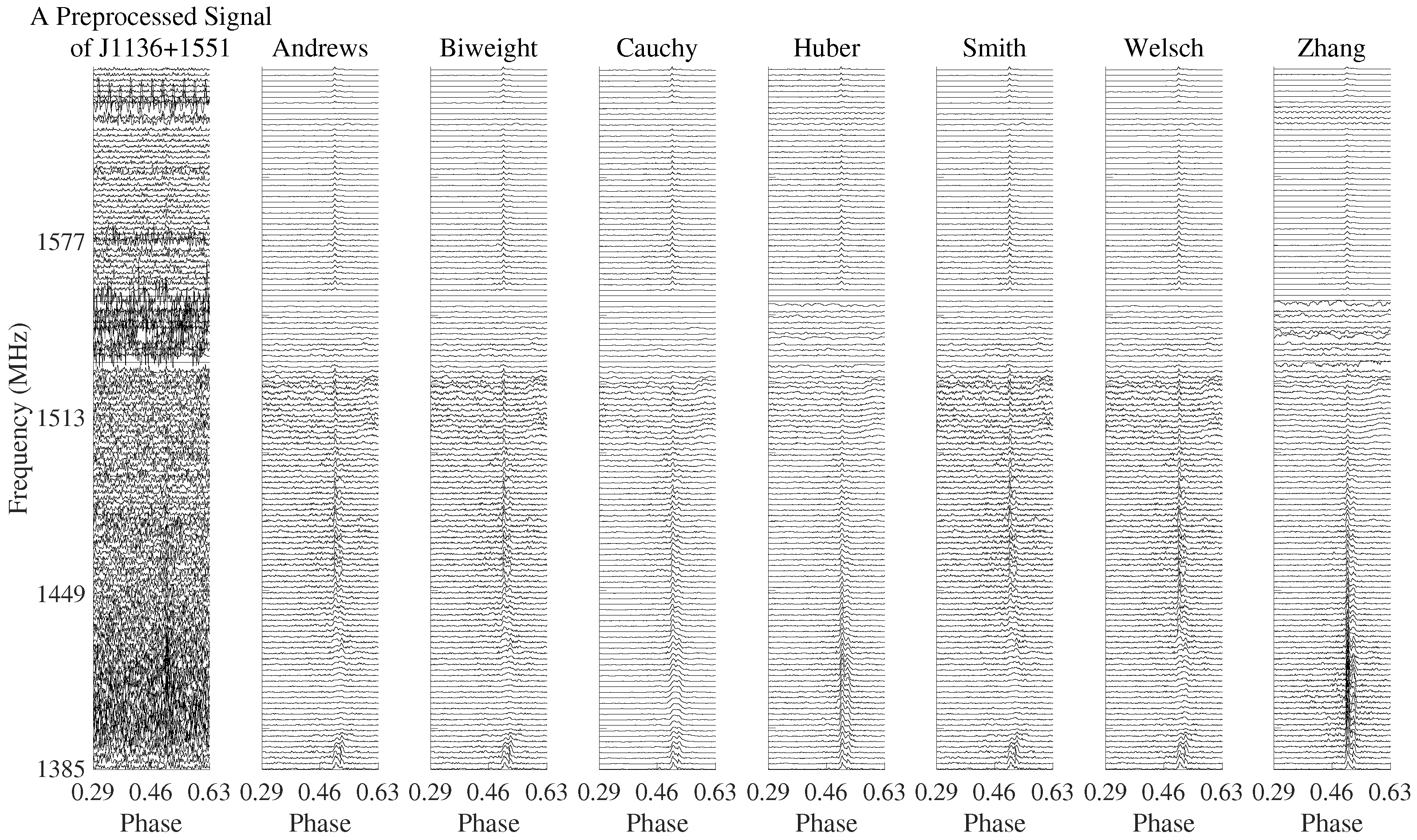
Figure 4.
RFI mitigation of a signal profile of J0814+7429 by the seven M-estimators.
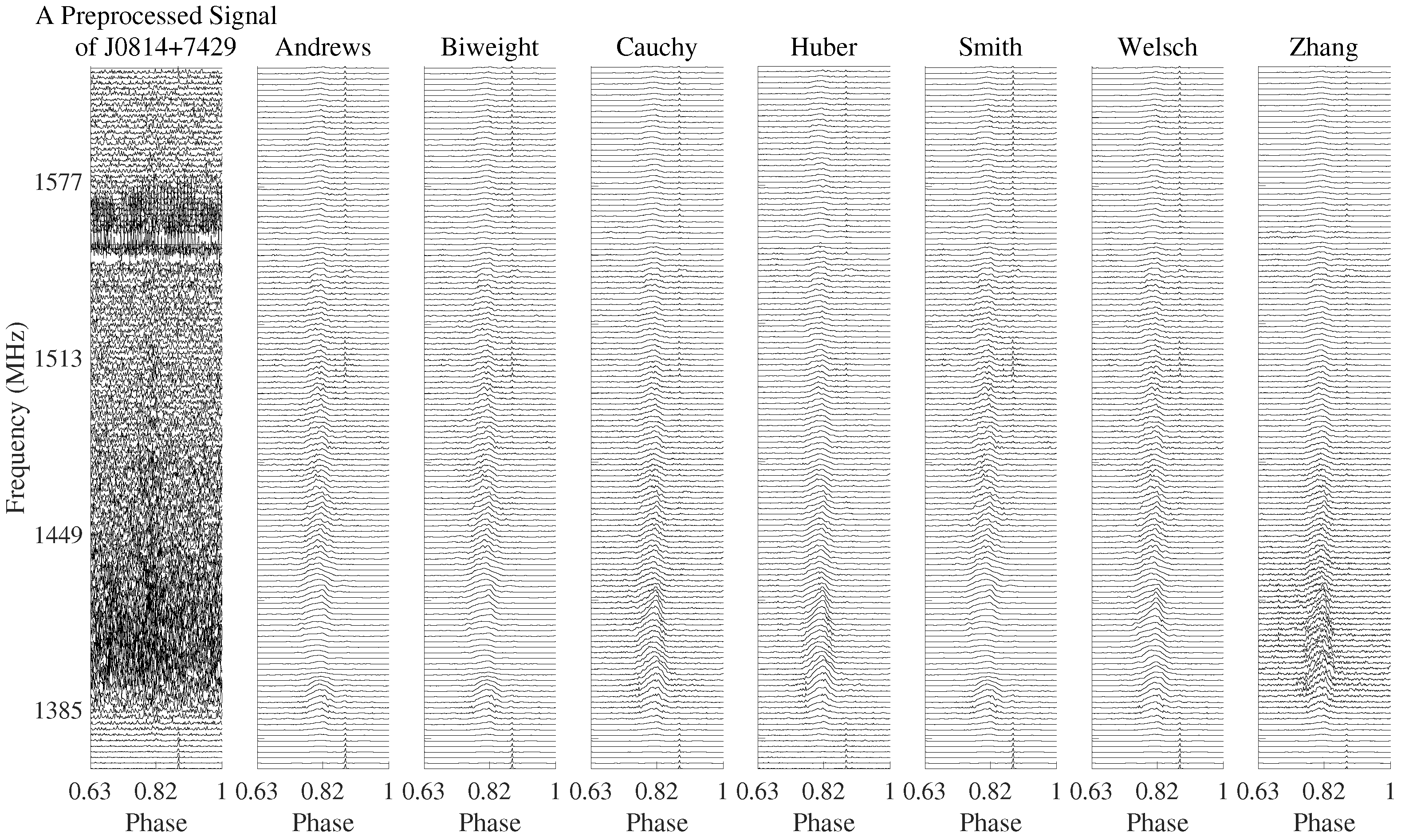
Figure 5.
RFI mitigation of a signal profile of J0332+5434 by the seven M-estimators.

Figure 6.
Dedispersed pulses of the processed profiles of J0332+5434 for a randomly selected band containing 50 consecutive channels. The seven estimators are applied, and the iteration steps are in the upper left corner of each panel.
Figure 6.
Dedispersed pulses of the processed profiles of J0332+5434 for a randomly selected band containing 50 consecutive channels. The seven estimators are applied, and the iteration steps are in the upper left corner of each panel.
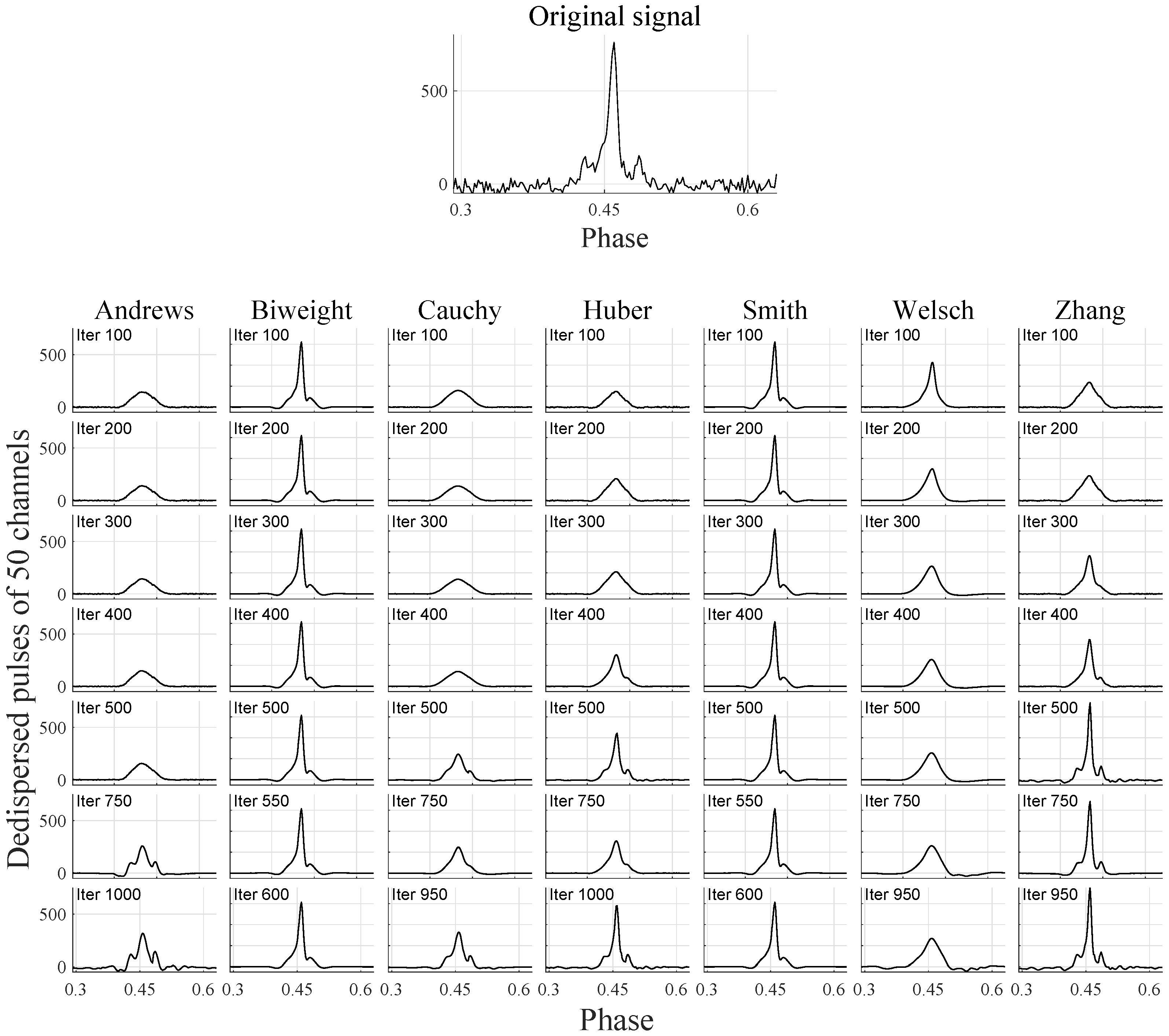
Figure 7.
RFI mitigation results for FRB 121102-11A with four resolutions (top) with the Huber estimator by the respective sparse transforms of curvelet (middle) and db8 wavelet (bottom).
Figure 7.
RFI mitigation results for FRB 121102-11A with four resolutions (top) with the Huber estimator by the respective sparse transforms of curvelet (middle) and db8 wavelet (bottom).

Figure 8.
Zooming-in details of the dedispersed dynamic spectra of two portions of the signals in Figure 7 with the sparse transforms of curvelet (top rows of (a,b)) and db8 wavelet (bottom rows of (a,b)).
Figure 8.
Zooming-in details of the dedispersed dynamic spectra of two portions of the signals in Figure 7 with the sparse transforms of curvelet (top rows of (a,b)) and db8 wavelet (bottom rows of (a,b)).

Figure 9.
Line plots for the dedispersed dynamic spectra of the two portions of FRB 121102-11A processed by the nonlinear robust framework applying the Huber estimator with curvelet (left panels of the top and bottom) and db8 wavelet (right panels of the top and bottom). The top and right subpanels show the 1D bursts as summed across frequencies and flattened spectra integrated in time.
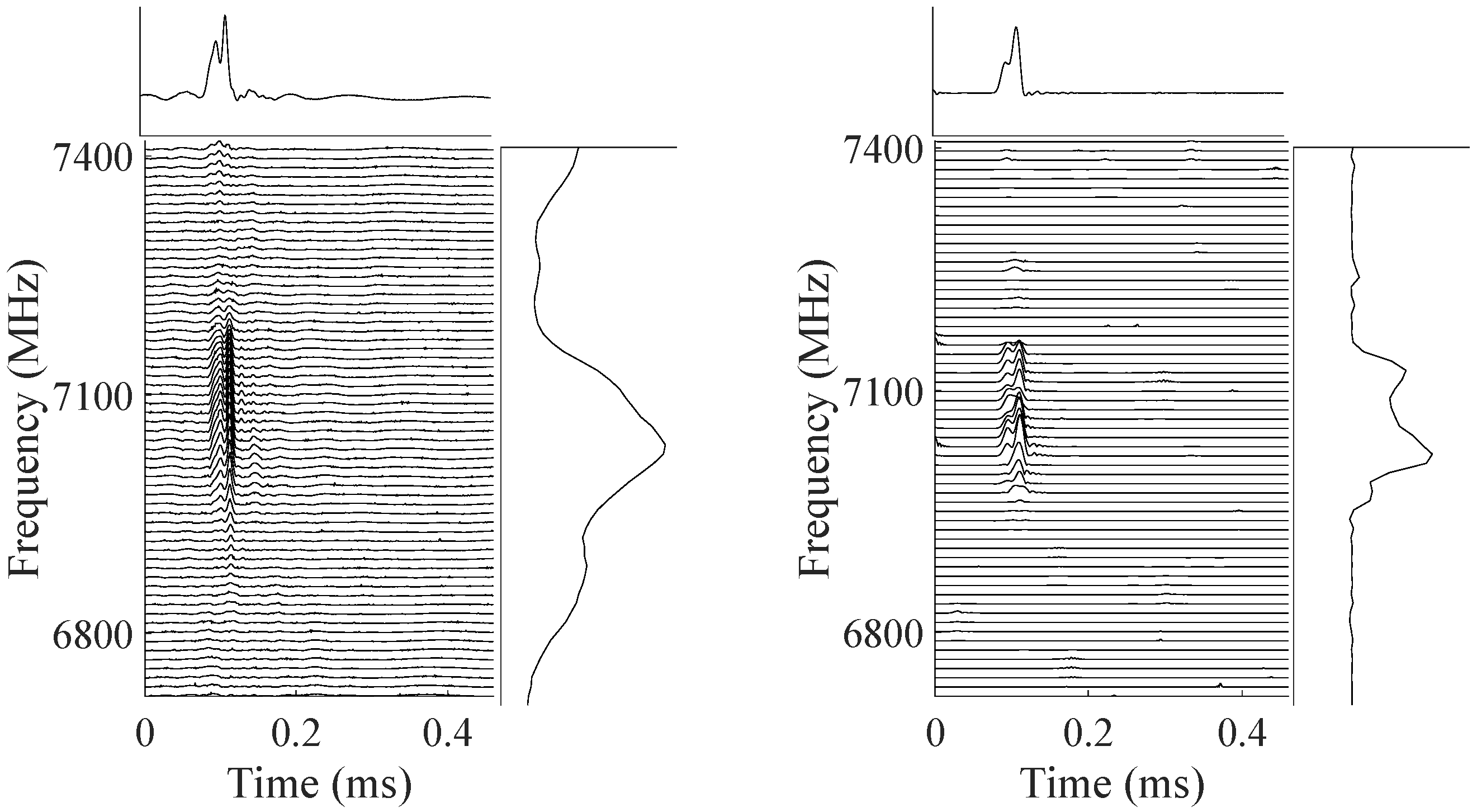
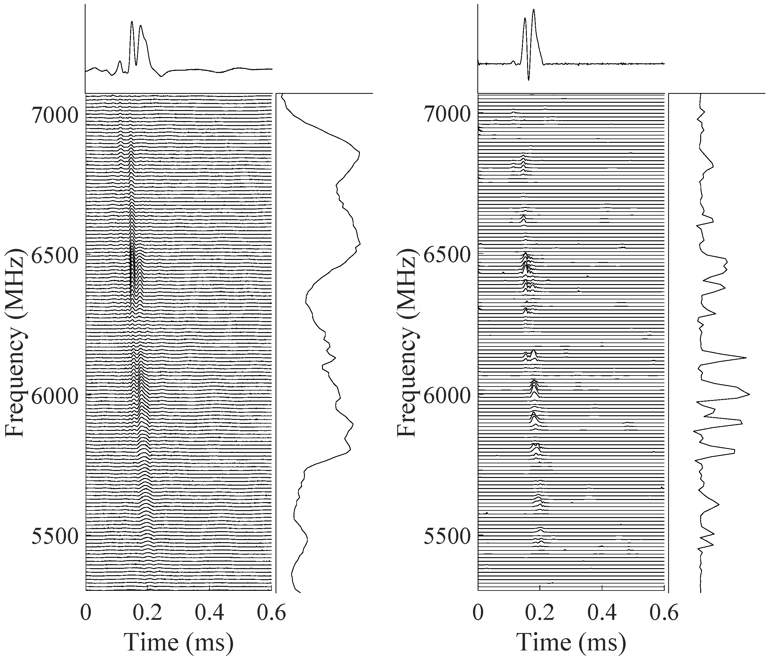
Figure 10.
A demonstration of the recognized flux regions in the two image portions by the db8 wavelet with the Cauchy, Huber, and Zhang estimators.
Figure 10.
A demonstration of the recognized flux regions in the two image portions by the db8 wavelet with the Cauchy, Huber, and Zhang estimators.


Table 1.
Robust M-estimators.
| M-Estimators | Functions | Tuning Parameters |
|---|---|---|
| Huber (monotone) | (x) = | |
| Zhang (monotone) | (x) = | |
| Cauchy (soft-redescending) | ||
| Welsch (soft-redescending) | (x) = | |
| Biweight (hard-redescending) | (x) = | |
| Andrews (hard-redescending) | (x) = | |
| Smith (hard-redescending) | (x) = |
Table 2.
A quantitative evaluation in terms of the SINR (in dB) for the seven M-estimators in RFI mitigation for PSRs J1645−0317, J1136+1551, J0814+7429, and J0332+5434.
Table 2.
A quantitative evaluation in terms of the SINR (in dB) for the seven M-estimators in RFI mitigation for PSRs J1645−0317, J1136+1551, J0814+7429, and J0332+5434.
| J1645−0317 | J1136+1551 | J0814+7429 | J0332+5434 | |
|---|---|---|---|---|
| Andrews | 1.73 | 1.63 | 4.40 | 2.11 |
| Biweight | 1.76 | 1.69 | 4.52 | 2.15 |
| Cauchy | 2.60 | 5.41 | 9.15 | 0.94 |
| Huber | 5.40 | 5.17 | 7.83 | 5.75 |
| Smith | 1.33 | 1.27 | 4.07 | 1.75 |
| Welsch | 2.37 | 2.42 | 7.60 | 2.79 |
| Zhang | 0.81 | 2.63 | 7.18 | 4.55 |
Table 3.
A quantitative evaluation of RFI mitigation efficacy in terms of the SINR (in dB) for FRB 121102-11A under four resolutions. The Huber estimator is applied.
Table 3.
A quantitative evaluation of RFI mitigation efficacy in terms of the SINR (in dB) for FRB 121102-11A under four resolutions. The Huber estimator is applied.
| Resolutions (MHz, s) | (0.86875, 10.1) | (1.7375, 20.2) | (3.475, 40.4) | (6.95, 80.8) |
|---|---|---|---|---|
| Signals | −26.5026 | −17.6826 | −6.6232 | −1.9036 |
| Results of curvelet | −8.5827 | 2.2026 | 8.4972 | 11.4321 |
| Results of db8 wavelet | −2.0663 | −0.6488 | −0.1546 | −0.0494 |
Table 4.
A quantitative evaluation in terms of the SINR (in dB) for seven M-estimators in RFI mitigation for FRB 121102-11A with six signal sizes.
Table 4.
A quantitative evaluation in terms of the SINR (in dB) for seven M-estimators in RFI mitigation for FRB 121102-11A with six signal sizes.
| Original | Andrews | Biweight | Cauchy | Huber | Smith | Welsch | Zhang | |
|---|---|---|---|---|---|---|---|---|
| 4096 × 2048 | −29.57 | −14.37 | −14.42 | −2.57 | −8.43 | −14.49 | −14.02 | −5.97 |
| 2048 × 1024 | −23.03 | −6.37 | −7.37 | −2.47 | 2.20 | −8.30 | −5.08 | 2.22 |
| 1024 × 512 | −16.77 | 5.63 | 5.73 | −2.46 | 8.50 | 5.63 | 2.84 | 7.76 |
| 512 × 256 | −11.52 | 8.03 | 8.04 | −2.41 | 11.43 | 8.04 | 8.15 | 11.12 |
| 256 × 128 | −6.93 | 8.25 | 8.22 | −2.48 | 10.03 | 8.19 | 8.21 | 10.02 |
| 128 × 64 | −1.63 | 9.64 | 9.50 | −2.60 | 10.26 | 9.52 | 9.66 | 10.18 |
Table 5.
Recognized isotropic flux regions by seven wavelets. The Cauchy, Huber, and Zhang estimators are applied.
Table 5.
Recognized isotropic flux regions by seven wavelets. The Cauchy, Huber, and Zhang estimators are applied.
| Wavelets | bior4.4 | coif5 | db8 | dmey | fk8 | rbio2.8 | sym8 |
|---|---|---|---|---|---|---|---|
| Cauchy | 10, 6 | 10, 10 | 8, 11 | 11, 11 | 8, 12 | 2, 1 | 9, 10 |
| Huber | 14, 12 | 15, 18 | 16, 19 | 15, 18 | 15, 19 | 9, 6 | 14, 17 |
| Zhang | 16, 6 | 16, 18 | 16, 18 | 15, 19 | 15, 20 | 11, 8 | 14, 19 |
Disclaimer/Publisher’s Note: The statements, opinions and data contained in all publications are solely those of the individual author(s) and contributor(s) and not of MDPI and/or the editor(s). MDPI and/or the editor(s) disclaim responsibility for any injury to people or property resulting from any ideas, methods, instructions or products referred to in the content. |
© 2023 by the authors. Licensee MDPI, Basel, Switzerland. This article is an open access article distributed under the terms and conditions of the Creative Commons Attribution (CC BY) license (https://creativecommons.org/licenses/by/4.0/).
Share and Cite
MDPI and ACS Style
Shan, H.; Jiang, M.; Yuan, J.; Yang, X.; Yan, W.; Wang, Z.; Wang, N. Sparsity and M-Estimators in RFI Mitigation for Typical Radio Astrophysical Signals. Universe 2023, 9, 488. https://doi.org/10.3390/universe9120488
AMA Style
Shan H, Jiang M, Yuan J, Yang X, Yan W, Wang Z, Wang N. Sparsity and M-Estimators in RFI Mitigation for Typical Radio Astrophysical Signals. Universe. 2023; 9(12):488. https://doi.org/10.3390/universe9120488
Chicago/Turabian StyleShan, Hao, Ming Jiang, Jianping Yuan, Xiaofeng Yang, Wenming Yan, Zhen Wang, and Na Wang. 2023. "Sparsity and M-Estimators in RFI Mitigation for Typical Radio Astrophysical Signals" Universe 9, no. 12: 488. https://doi.org/10.3390/universe9120488
Note that from the first issue of 2016, this journal uses article numbers instead of page numbers. See further details here.