Line Shapes in a Magnetic Field: Trajectory Modifictions II: Full Collision-Time Statistics

Abstract

In a previous paper, a variation of the Collision-time Statistics method was applied to identify the relevant perturbers for line broadening under the action of a constant magnetic field. As discussed, that version was simplified and inadequate for low magnetic field and/or large perturber mass (ions). The purpose of the present work is to augment the previous work, so that such cases can be handed efficiently. The results may also be used to construct analytic, i.e., impact/unified models under the usual assumptions in these models.

1. Introduction

In a previous paper [1], a variation of the Collision-time Statistics method was applied to identify the relevant perturbers for line broadening under the action of a constant magnetic field. As discussed, that version was simplified and inefficient for low magnetic field and/or or large perturber mass (ions), because an unnecessarily large number of perturbers, the vast majority of which only contribute negligibly to broadening, were generated. The purpose of the present work is to augment the previous work, so that such cases can be handled efficiently. The main problem with the previous treatment was the case of large Larmor radii and corresponding slow cyclotron frequencies, as in the case of large perturber mass and/or low magnetic field. In such cases the motion of the perturbers in the plane perpendicular to the magnetic field may be quite far from completing a full cycle. As a result in the simplified treatment of [1] a large number of ineffective perturbers would be included in that case. It is believed [2] that “as long as the gyro-radii of the electrons are much larger than the Debye sphere” the particle trajectories, or, equivalently, the dielectric function would be unaffected by the magnetic field, since the perpendicular motion involves presumably much smaller length scales than the parallel motion, although this belief remains to be quantified. It is shown here that this criterion is not quite correct and that the key parameter determining the adequacy of neglecting spiralling is the ratio of the cyclotron frequency to the width of the line in question.

2. Theoretical Formulation

As in [1] we assume that:

• the distribution functions, e.g., the Maxwellian velocity distribution is $not$ affected by the B-field.
• the shielding is also not affected, e.g., Debye screening

We also consider a neutral emitter in this work.

2.1. Collision-Time Statistics

To include $all$ and only the relevant perturbers, we use a modification of the collision-time statistics method of Hegerfeld and Kesting [3] with Seidel’s improvement [4]- see Ref. [5] for details, as discussed in [1].

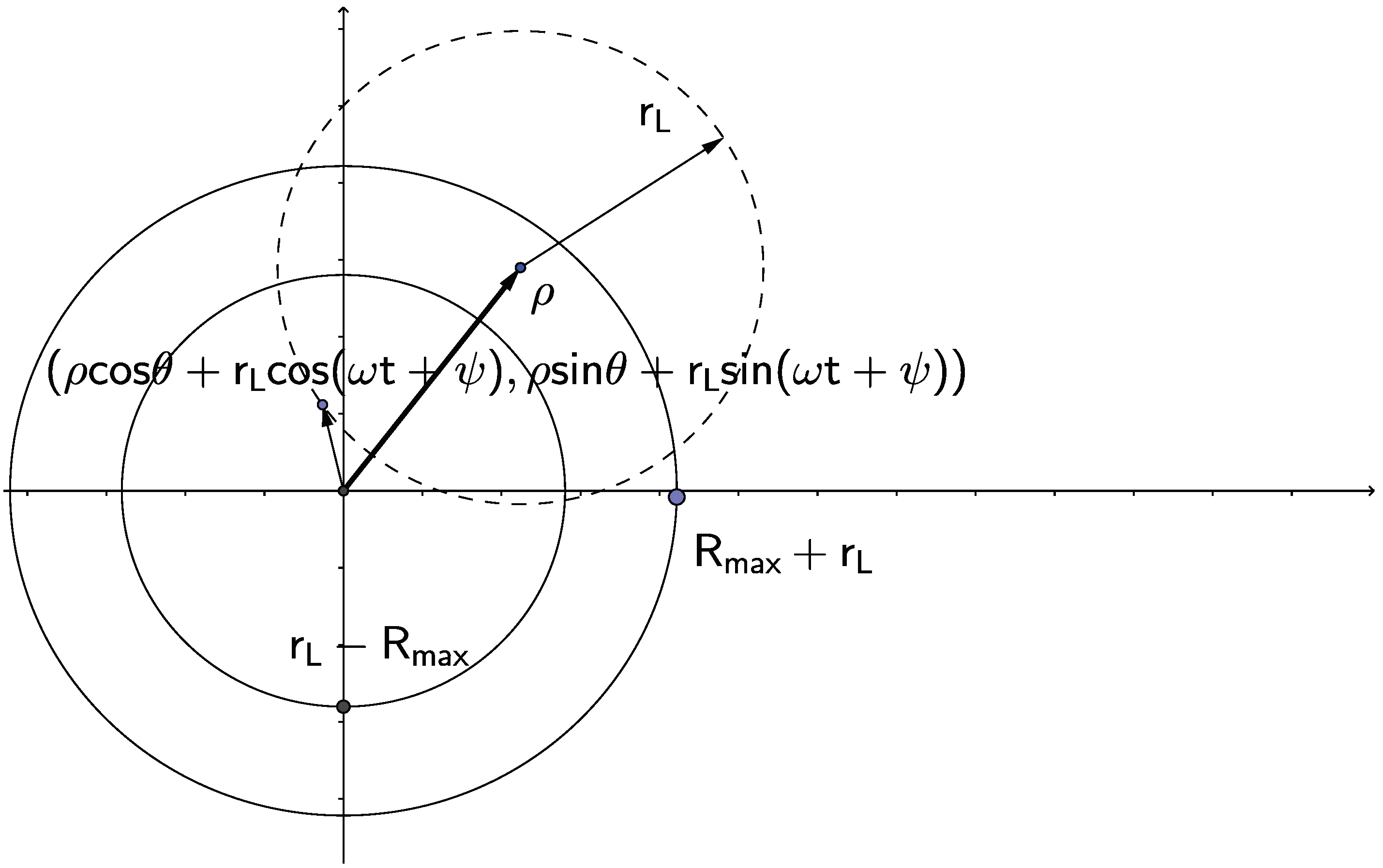
As in [1], perturbers move in a helical path characterized by the parallel constant velocity $v_z$, where the magnetic field direction defines the z-axis (passing through the emitter), the perpendicular velocity with magnitude $v_{\perp }$ and impact parameter $\rho$, which is the distance of the center of the spiral to the z-axis, i.e., the perpendicular motion in the x-y plane is a circular motion with the Larmor radius $r_L=\frac{v_{\perp }}{{\omega }_L}$ around the center $\rho$, with ${\omega }_L=|Q|B/m$ the cyclotron frequency and Q the perturber charge. For the impact parameter $\rho$

$$max(0,r_L-R_{max})\le \rho \le R_{max}+r_L,$$

(1)

i.e., the impact parameter lies in a disk or annulus depending on whether the range $R_{max}$ of the interaction, discussed below, is larger or smaller than $r_L$.

The relevant quantities for the helical trajectory R(t) are as follows: The z-coordinate of the trajectory is

$$R_z(t)=v_z(t-t_i)=v_{z}t+z_0,$$

(2)

with

$$z_0=-v_z{t}_i,$$

(3)

with the times of closest approach $t_i$ representing the time the perturber trajectory intersects the x-y plane and being uniformly distributed. $z_0$ thus represents how far from the x-y plane the perturber is at t = 0.

Hence

$$R_x(t)=\rho cos\theta +r_{L}cos({\omega }_{L}t+\psi ),R_y(t)=\rho sin\theta +r_{L}sin({\omega }_{L}t+\psi )$$

(4)

where $\theta$ describes the position of the impact parameter vector in the x-y plane and is uniformly distributed in ($0,2\pi$). $\psi$ is an angle describing where on the circular trajectory projection the perturber finds itself at $t=0$ and is also uniformly distributed in ($0,2\pi$) and ultimately related to the time the B-field was turned on. Each perturber is thus characterized by the vector $(v_z,v_{\perp },\rho ,\theta ,\psi ,t_i)$, or equivalently $z_0$ instead of $t_i$.

As in [1] we consider as “relevant " perturbers those that, at any time during the interval of interest (0,$\tau$), come closer to the emitter than a distance $R_{max}$, defined so that the interaction is negligible for distances larger than $R_{max}$. For a Debye interaction, we usually take $R_{max}\approx 3{\lambda }_D$, where ${\lambda }_D$ denotes the shielding(Debye) length. This is because the interation becomes negligible ($\le 3\%$ for larger distances).

Therefore for a perturber to be relevant the condition $R(t)\le R_{max}$ must hold for at least one time t in $(0,\tau )$, where $\tau$ is the time of interest, i.e., a time large enough that the Fourier transform of the line profile $C(t)$ has decayed to negligible levels, or an asymptotic form is identifiable. $C(t)$ is a linear combination of products of time evolution operators (U-matrices) of the upper and lower levels. These time evolution operators -needed for times $0\le t\le \tau$- are determined by solving the Schroedinger equation in the Debye-shielded field $V(t)$. Therefore a particle will only be relevant if for at least one time in the interval [0,$\tau$] it comes closer than $R_{max}$ to the emitter(if not, then the perturbation produced by that particle is negligible due to Debye screening), which means that for at least $one$ time t in [0,$\tau$]:

$${(v_{z}t+z_0)}^2+{(\rho cos\theta +r_{L}cos({\omega }_{L}t+\psi ))}^2+{(\rho sin\theta +r_{L}sin({\omega }_{L}t+\psi ))}^2\le R_{max}^2$$

(5)

This reads:

$$R_{max}^2-{(v_{z}t-v_z{t}_i)}^2\ge {\rho }^2+r_L^2+2\rho r_{L}cos({\omega }_{L}t+\psi -\theta )$$

(6)

Thus we generate $v_z,v_{\perp },\rho ,t_i$ and $\theta$ as before, but also draw $\psi$, uniformly distributed in ($0,2\pi )$ as illustrated in in Figure 1 and effectively only accept perturbers if, for at least one time in (0,$\tau$) Equation (6) is satisfied. The $maximum$ value of the LHS occurs for $t=t_i$. This in general imposes $restrictions$ (i.e., not all $\psi$ contribute for a given $\theta$) on the values of $\theta$ and $\psi$ that a perturber can have and still contribute effectively to broadening, specifically:

Figure 1. x-y trajectory projections for $r_L\ge R_{max}$. Shown is the annular region between concentric circles with the origin (the emitter position) as center and radii $r_L-R_{max}$ and $r_L+R_{max}$, respectively. For an impact parameter at a distance $\rho$ from the center in the annular region, a circle with radius $r_L$ (dashed) represents the projection of the perturber path in the x-y plane. Hence a point on that circle is $\left(\rho cos\theta +r_{L}cos(\omega t+\psi ),\rho sin\theta +r_{L}sin(\omega t+\psi )\right)$, with $\psi$ the angle on the dashed circle. This must be no more than $R_{max}$ away from the center, else this perturber does not contribute.

• If $r_L<R_{max}$ and $\rho \le R_{max}-r_L$, $R_{max}\ge \rho +r_L$ and Equation (6) is satisfied for $t=t_i$ for $any$ $\theta ,\psi$ and ${\omega }_{L}t$. Therefore in this case we have no restriction and $\theta$ and $\psi$ can independently take any value.
• In all other cases, Equation (6) results in the restriction:

  $$arccos(\frac{R_{max}^2-{\rho }^2-r_L^2}{2\rho r_L})\le |{\omega }_{L}t+\psi -\theta |$$

  (7)

Note that for Case b, the argument of the inverse cosine is absolutely ≤1. Specifically:

• If $r_L\ge R_{max}$, then

  $$0\ge \frac{R_{max}^2-r_L^2-{\rho }^2}{2\rho r_L}\ge -1$$

  (8)
  The left of the inequality follows because $R_{max}\le r_L$ alone. The right part also follows since

  $$r_L-R_{max}\le \rho \le r_L+R_{max}\Rightarrow -R_{max}\le \rho -r_L\le R_{max}$$

  (9)
  Hence

  $$R_{max}^2\ge {\rho }^2+r_L^2-2\rho r_L\Rightarrow \frac{R_{max}^2-r_L^2-{\rho }^2}{2\rho r_L}\ge -1$$

  (10)
• For $r_L\le R_{max}$, Equation (9) is also valid since $r_L-R_{max}\le 0\le \rho$, as is Equation (10). Since, as already discussed the case $\rho \le R_{max}-r_L$ imposes no restriction, we only consider here the case $R_{max}-r_L\le \rho \le R_{max}+r_L$, which implies $\rho -r_L\le R_{max}\le \rho +r_L$. It thus remains to show that

  $$\frac{R_{max}^2-r_L^2-{\rho }^2}{2\rho r_L}\le 1$$

  (11)

  which follows from $R_{max}\le \rho +r_L$.

Thus

• For $r_L\le R_{max},\rho \le r_L$, Equation (6) is satisfied for $t=t_i$ for any $\theta ,\psi$ and ${\omega }_{L}t$ and there is no restriction on $\psi ,\theta$ and ${\omega }_{L}t$.
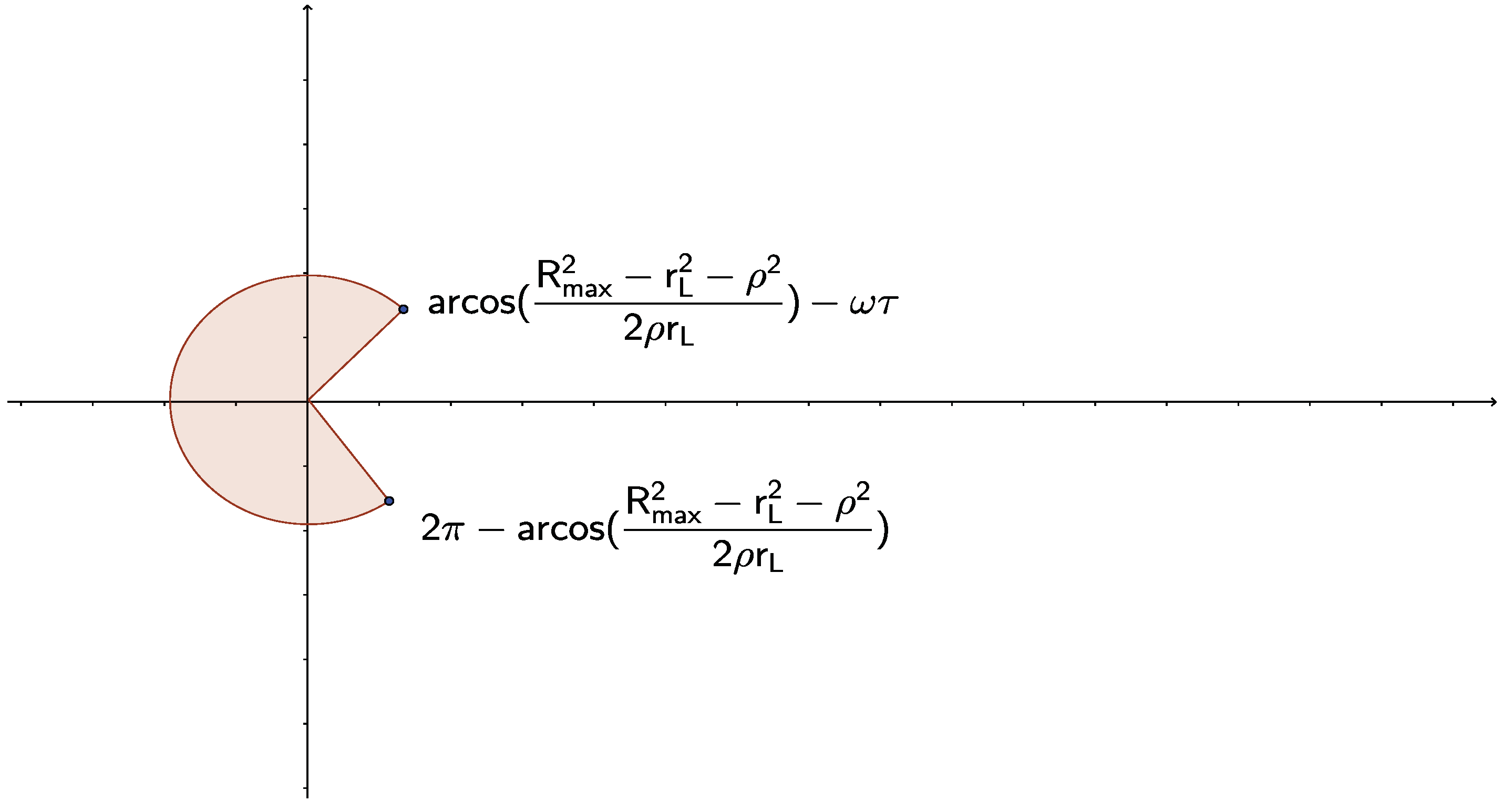
• In all other cases, the restriction imposed by Equation (7) applies and the argument of the inverse cosine is always absolutely $\le 1$.

Hence the angle difference $\psi -\theta$ must be in the shaded area shown in Figure 2. So for at least one time t in ($0,\tau$), the following must hold for the perturber with parameters $\rho ,r_L,\theta ,\psi$ to contribute:

$$|\psi +{\omega }_{L}t-\theta |\ge arccos(\frac{R_{max}^2-{\rho }^2-r_L^2}{2\rho r_L}).$$

(12)

i.e.,

$$\psi +{\omega }_{L}t\ge \theta +arccos(\frac{R_{max}^2-{\rho }^2-r_L^2}{2\rho r_L}),\psi +{\omega }_{L}t\ge \theta$$

(13)

or

$$\theta -arccos(\frac{R_{max}^2-{\rho }^2-r_L^2}{2\rho r_L})\ge \psi +{\omega }_{L}t,\theta \ge \psi +{\omega }_{L}t$$

(14)

Figure 2. The shaded area shows the difference $\psi -\theta$ that satisfies Equation (6).

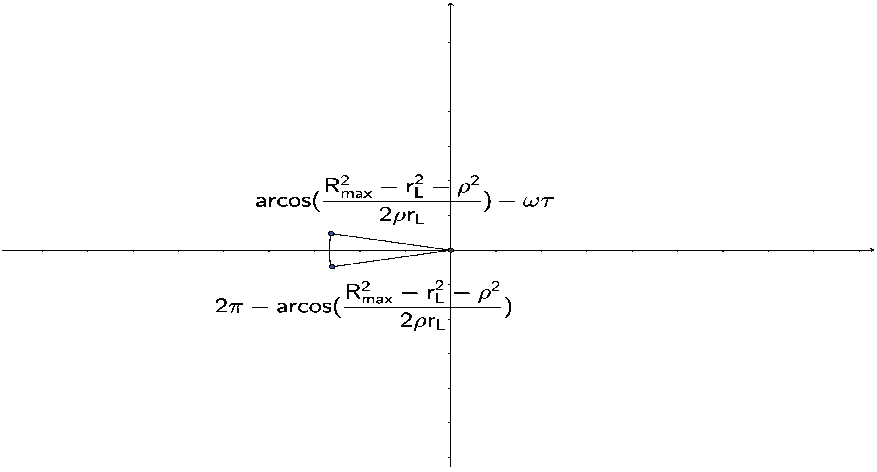
The net result is that for each $\theta$, only a a range of $\psi$,

$$\Delta \psi \le 2\left(\pi -arccos(\frac{R_{max}^2-{\rho }^2-r_L^2}{2\rho r_L})\right)+{\omega }_L\tau$$

(15)

contributes (this means that a fraction $\frac{\Delta \psi }{2\pi }$ contributes compared to the simplified case discussed in the previous work, i.e., the collision volume is smaller by $\frac{\Delta \psi }{2\pi }$). If this is $\ll 1$ we effectively have rectilinear trajectories for the time of interest. If this turns out to be larger than $2\pi$, we have a full revolution and we can use the simplified formulas discussed in [1]. As mentioned, we are mainly interested in the situation where $R_{max}<r_L$ and ${\omega }_L\tau <2\pi$, as this is the case of large $r_L$, but slow ${\omega }_L$, otherwise the relation between $\psi$ and $\theta$ is always satisfied for at least one t in $(0,\tau )$.

We can use the variable $x=\rho -r_L$ with $-R_{max}\le x\le R_{max}$ and write the argument of the inverse cosine as

$$\frac{R_{max}^2-{\rho }^2-r_L^2}{2\rho r_L}=\frac{R_{max}^2-x^2}{2r_L(x+r_L)}-1$$

(16)

Note that for low B (large $r_L$) this tends to −1, hence the inverse cosine is close to $\pi$. This means that in this limit $|\psi -\theta |\approx \pi$, e.g., we get a $\Delta \psi \approx 0$ (but note that in that limit we had divergencies in the relevant functions when computing the collision volume in [1]).

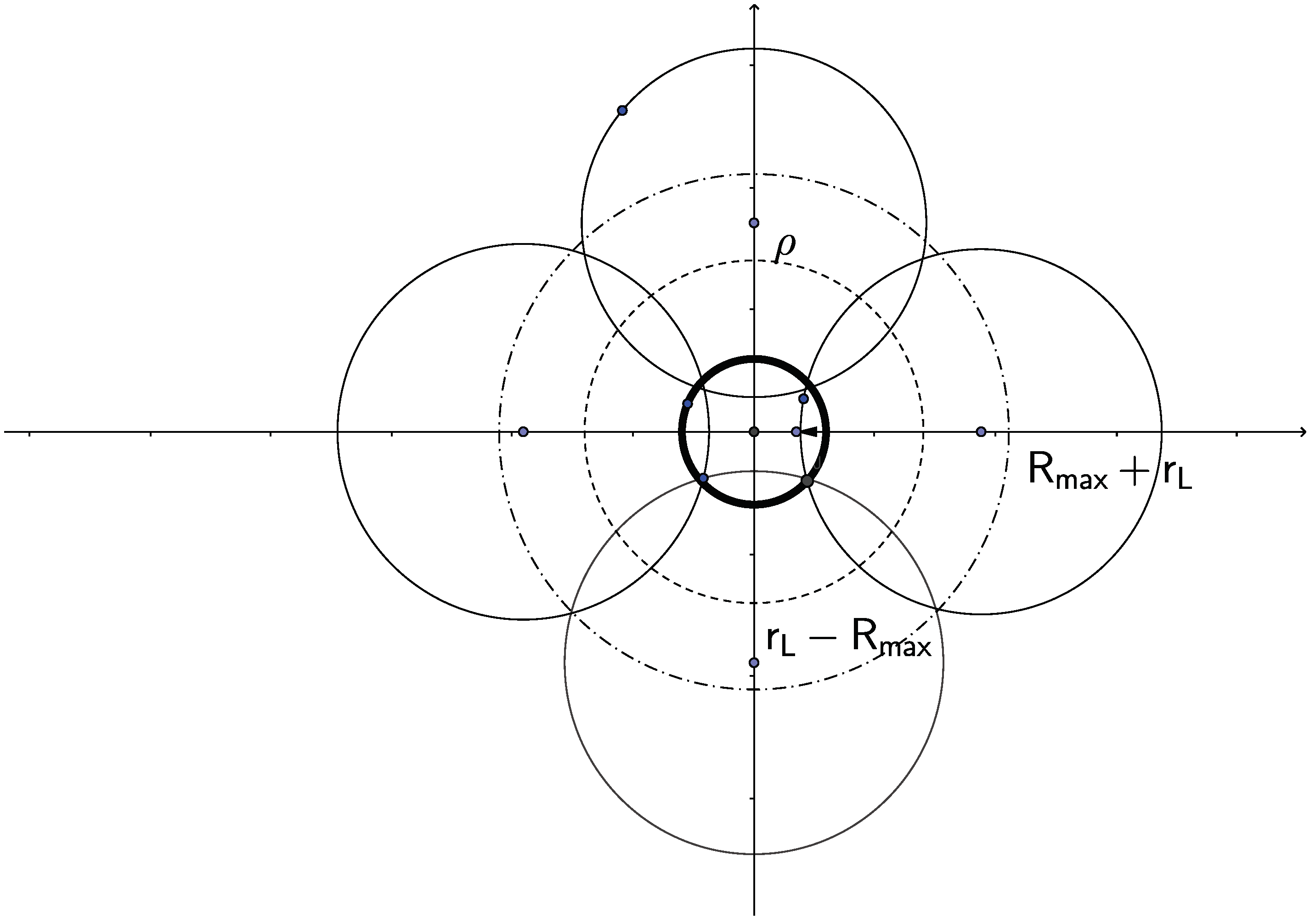
This situation is depicted in Figure 3, which shows the typical situation for the phase space of the quantity $\psi -\theta$ that contributes. This is also illustrated in Figure 4, which shows, for the same $\rho$, 4 different angles $\theta$, which determine the centers of the spirals and the parts of the circular projections of these spirals that are effective. For instance if the center of the spiral, i.e., the vector of the impact parameter is the the right ($\theta \approx 0$), then $\psi \approx \pi$ (the leftmost of the circular trajectory projection) for $r_L\gg R_{max}$. Similarly, if the impact parameter vector is to the south ($\theta \approx 3\pi /2$), then the relevant $\psi$ is to the north of the circular trajectory projection, e.g., $\psi \approx \pi /2$).

Figure 3. The shaded area shows the difference $\psi -\theta$ that satisfies Equation (6).

Figure 4. Illustration of the relation between $\theta$ and $\psi$ for the case $r_L\gg R_{max}$. Impact parameters $\rho$ lie between the dashed and dash-dotted circles with radii $r_L-R_{max}$ and $r_L+R_{max}$. The part of the circular trajectory projections that are within $R_{max}$(bold circle) of the emitter (i.e., the center) are in the opposite direction of the impact parameter vector, e.g., to the north for the southern circular trajectory projection.

In the limit $B=0$ (or infinite perturber mass), $arccos(\frac{R_{max}^2-{\rho }^2-r_L^2}{2\rho r_L})=\pi$ and we get from the $\theta$ and $\psi$ integrations a term $\frac{{\omega }_L\tau }{2\pi }$.

2.2. Collision Volume

The collision-time statistics method first computes the number of relevant particles, i.e., the density times the relevant volume, i.e., the above cylinder. This volume is as before [1], except that we also account for the polar angle $\theta$, describing the orientation of the impact parameter with respect to the x-axis and the angle $\psi$ describing the position of the particle on the perpendicular x-y plane at time $t=0$, i.e., we have the extra integrations ${\int }_0^{2\pi }\frac{d\theta }{2\pi }{\int }_0^{2\pi }\frac{d\psi }{2\pi }$. The $\psi$ integration simply returns a factor of 1 if ${\omega }_L\tau \ge 2\pi$, but it does so even under the weaker condition ${\omega }_L\tau \ge 2arccos(\frac{R_{max}^2-{\rho }^2-r_L^2}{2\rho r_L})$, or

$$\frac{R_{max}^2-{\rho }^2-r_L^2}{2\rho r_L}\ge cos({\omega }_L\tau /2)$$

(17)

Otherwise it gives a factor of $\frac{\Delta \psi }{2\pi }$ with $\Delta \psi$ defined in Equation (15).

The nonnegative root of Equation (17) is

$${\rho }_1=-cos({\omega }_L\tau /2)r_L+\sqrt{R_{max}^2-{sin}^2({\omega }_L\tau /2)r_L^2},$$

(18)

i.e., the results of [1] are also valid for $\rho \le {\rho }_1$, which in turn requires that

$$R_{max}>r_L$$

(19)

(else ${\rho }_1\le 0$), which also guarantees the reality of ${\rho }_1$, i.e.,

$$R_{max}\ge sin({\omega }_L\tau /2)r_L$$

(20)

The $\theta$ angular integration simply returns 1 in either case. As a result, the results of [1] need $no$ $modification$ for ${\omega }_L\tau \ge 2\pi$. Otherwise, the collision volume calculation runs as follows:

For $v_{\perp }<R_{max}{\omega }_L$, i.e., $r_L<R_{max}$, $\Delta \psi (\rho )=1$. However, as already discussed, this is valid (e.g., no restriction on $\psi$ is required ) also for $\rho <r_L$, hence $\Delta \psi (\rho )=1$ for $\rho \le max(r_L,{\rho }_1)={\rho }_2$.

For small $R_{max}/r_L$ and ${\omega }_L\tau ,r_L$ is the maximum of the two. The collision volume reads:

$$\begin{array}{c}V=2\pi {\int }_{-\infty }^{\infty }f(v_z)d{v}_z{\int }_0^{\infty }{f}_2(v_{\perp })d{v}_{\perp }{\int }_{max(0,\frac{v_{\perp }}{{\omega }_L}-R_{max})}^{R_{max}+\frac{v_{\perp }}{{\omega }_L}}\rho d\rho \Delta \psi (\rho ){\int }_{-\frac{\sqrt{R_{max}^2-{(\rho -r_L)}^2}}{|v_z|}}^{\tau +\frac{\sqrt{R_{max}^2-{(\rho -r_L)}^2}}{|v_z|}}d{t}_i\end{array}$$

(21)

$$\begin{array}{c}=2\pi {\int }_{-\infty }^{\infty }f(v_z)d{v}_z{\int }_0^{\infty }{f}_2(v_{\perp })d{v}_{\perp }{\int }_{max(0,\frac{v_{\perp }}{{\omega }_L}-R_{max})}^{R_{max}+\frac{v_{\perp }}{{\omega }_L}}(|v_z|\tau +2\sqrt{R_{max}^2-{(\rho -r_L)}^2})\Delta \psi (\rho )\rho d\rho \\ =2\pi (C_1+C_2)\end{array}$$

with $f(v_z)=\sqrt{\frac{m}{2\pi kT}}{e}^{-m{v}_z^2/2kT}$ and $f_2(v_{\perp })=\frac{m}{kT}{v}_{\perp }{e}^{-m{v}_{\perp }^2/2kT}$ denoting a one and two-dimensional Maxwellian velocity distributions respectively and with $\Delta \psi$ redefined as in Table 1:

Table 1. $\frac{\Delta \psi (\rho )}{2\pi }$ vs. relevant parameters.

${\mathit{\omega }}_{\mathit{L}}\mathit{\tau }$	$\frac{{\mathit{r}}_{\mathit{L}}}{{\mathit{R}}_{\mathit{max}}}$	$\frac{\mathit{\rho }}{\mathit{max}({\mathit{\rho }}_1,{\mathit{r}}_{\mathit{L}})}$	$\frac{\mathbf{\Delta }\mathit{\psi }(\mathit{\rho })}{2\mathit{\pi }}$
$\ge 2\pi$			1
$<2\pi$	$\le 1$	$\le 1$	1
$<2\pi$	$\le 1$	$>1$	$\left(1-\frac{arccos(\frac{R_{max}^2-{\rho }^2-r_L^2}{2\rho r_L})}{\pi }\right)+\frac{{\omega }_L\tau }{2\pi }$
$<2\pi$	$>1$		$\left(1-\frac{arccos(\frac{R_{max}^2-{\rho }^2-r_L^2}{2\rho r_L})}{\pi }\right)+\frac{{\omega }_L\tau }{2\pi }$

$C_1$ and $C_2$ are:

$$\begin{array}{cc}{C}_1\hfill & =\tau {\int }_{-\infty }^{\infty }f(v_z)|v_z|d{v}_z{\int }_0^{\infty }{f}_2(v_{\perp })d{v}_{\perp }{\int }_{max(0,\frac{v_{\perp }}{{\omega }_L}-R_{max})}^{R_{max}+\frac{v_{\perp }}{{\omega }_L}}\rho d\rho \Delta \psi (\rho )\hfill \\ & =⟨|v_z|⟩\tau {\int }_0^{\infty }{f}_2(v_{\perp })d{v}_{\perp }{\int }_{max(0,\frac{v_{\perp }}{{\omega }_L}-R_{max})}^{R_{max}+\frac{v_{\perp }}{{\omega }_L}}\rho d\rho \Delta \psi (\rho )\hfill \\ & =⟨|v_z|⟩\tau [{\int }_0^{R_{max}{\omega }_L}{f}_2(v_{\perp })d{v}_{\perp }{\int }_0^{R_{max}+\frac{v_{\perp }}{{\omega }_L}}\rho d\rho \Delta \psi (\rho )+{\int }_{R_{max}{\omega }_L}^{\infty }{f}_2(v_{\perp })d{v}_{\perp }{\int }_{\frac{v_{\perp }}{{\omega }_L}-R_{max}}^{R_{max}+\frac{v_{\perp }}{{\omega }_L}}\rho d\rho \Delta \psi (\rho )]\hfill \\ & =⟨|v_z|⟩\tau R_{max}^2(I_1+I_2+I_3)\hfill \end{array}$$

(22)

with $⟨|v_z|⟩={\int }_{-\infty }^{\infty }|v|f(v)dv=\sqrt{\frac{2kT}{\pi m}}$ The integrals $I_1-I_3$ are given explicitly below. However, we first define the dimensionless quantities:

$$s=\frac{v_{\perp }}{{\omega }_L{R}_{max}}$$

(23)

and

$$r=\frac{{\rho }_2}{R_{max}}=max(-cos({\omega }_L\tau /2)s+\sqrt{1-{sin}^2({\omega }_L\tau /2)s^2},s)$$

(24)

and

$$q=R_{max}{\omega }_L\sqrt{\frac{m}{2kT}}$$

(25)

(essentialy the averaged inverse s $R_{max}/r_L$).

$$I_1=R_{max}^{-2}{\int }_0^{R_{max}{\omega }_L}{f}_2(v_{\perp })d{v}_{\perp }{\int }_0^{{\rho }_2}\rho d\rho ={\int }_0^{R_{max}{\omega }_L}{f}_2(v_{\perp })d{v}_{\perp }\frac{{\rho }_2^2(v_{\perp })}{2}$$

(26)

$$I_2=R_{max}^{-2}{\int }_0^{R_{max}{\omega }_L}{f}_2(v_{\perp })d{v}_{\perp }{\int }_{{\rho }_2}^{R_{max}+\frac{v_{\perp }}{{\omega }_L}}\rho (\left(1-\frac{arccos(\frac{R_{max}^2-{\rho }^2-r_L^2}{2\rho r_L})}{\pi }\right)+\frac{{\omega }_L\tau }{2\pi })d\rho$$

(27)

and

$$I_3=R_{max}^{-2}{\int }_{R_{max}{\omega }_L}^{\infty }{f}_2(v_{\perp })d{v}_{\perp }{\int }_{\frac{v_{\perp }}{{\omega }_L}-R_{max}}^{R_{max}+\frac{v_{\perp }}{{\omega }_L}}\rho (\left(1-\frac{arccos(\frac{R_{max}^2-{\rho }^2-r_L^2}{2\rho r_L})}{\pi }\right)+\frac{{\omega }_L\tau }{2\pi })d\rho$$

(28)

while

$$\begin{array}{cc}{C}_2\hfill & =2{\int }_{-\infty }^{\infty }f(v_z)d{v}_z{\int }_0^{\infty }{f}_2(v_{\perp })d{v}_{\perp }{\int }_{max(0,\frac{v_{\perp }}{{\omega }_L}-R_{max})}^{R_{max}+\frac{v_{\perp }}{{\omega }_L}}\sqrt{R_{max}^2-{(\rho -r_L)}^2}\rho d\rho \Delta \psi (\rho )\hfill \\ \hfill & =2{\int }_0^{\infty }{f}_2(v_{\perp })d{v}_{\perp }{\int }_{max(0,\frac{v_{\perp }}{{\omega }_L}-R_{max})}^{R_{max}+\frac{v_{\perp }}{{\omega }_L}}\sqrt{R_{max}^2-{(\rho -r_L)}^2}\rho d\rho \Delta \psi (\rho )\hfill \\ \hfill & =2[{\int }_0^{R_{max}{\omega }_L}{f}_2(v_{\perp })d{v}_{\perp }{\int }_0^{R_{max}+\frac{v_{\perp }}{{\omega }_L}}\sqrt{R_{max}^2-{(\rho -r_L)}^2}\rho d\rho \Delta \psi (\rho )\hfill \\ \hfill & +{\int }_{R_{max}{\omega }_L}^{\infty }{f}_2(v_{\perp })d{v}_{\perp }{\int }_{\frac{v_{\perp }}{{\omega }_L}-R_{max}}^{R_{max}+\frac{v_{\perp }}{{\omega }_L}}\sqrt{R_{max}^2-{(\rho -r_L)}^2}\rho d\rho \Delta \psi (\rho )]\hfill \\ \hfill & =2R_{max}^3(J_1+J_2+J_3)\hfill \end{array}$$

(29)

with

$$\begin{array}{cc}{J}_1\hfill & =R_{max}^{-3}{\int }_0^{R_{max}{\omega }_L}{f}_2(v_{\perp })d{v}_{\perp }{\int }_0^{{\rho }_2}\sqrt{R_{max}^2-{(\rho -r_L)}^2}\rho d\rho \hfill \\ \hfill & ={\int }_0^{q^2}dx{e}^{-x}[\frac{s}{2}(arcsin(s)-arcsin(s-r))+\frac{(s^2+2)\sqrt{1-s^2}-(s^2+2+sr-2r^2)\sqrt{1-s^2+2sr-r^2}}{6}]\hfill \end{array}$$

(30)

with $x=\frac{m{v}_{\perp }^2}{2kT}$ and $s=\frac{x^{1/2}}{q},r$ being of course functions of x.

$$J_2=R_{max}^{-3}{\int }_0^{R_{max}{\omega }_L}{f}_2(v_{\perp })d{v}_{\perp }{\int }_{{\rho }_2}^{R_{max}+\frac{v_{\perp }}{{\omega }_L}}\sqrt{R_{max}^2-{(\rho -r_L)}^2}\rho \left(1-\frac{arccos(\frac{R_{max}^2-{\rho }^2-r_L^2}{2\rho r_L})}{\pi }\right)+\frac{{\omega }_L\tau }{2\pi })d\rho$$

(31)

and

$$J_3=R_{max}^{-3}{\int }_{R_{max}{\omega }_L}^{\infty }{f}_2(v_{\perp })d{v}_{\perp }{\int }_{\frac{v_{\perp }}{{\omega }_L}-R_{max}}^{R_{max}+\frac{v_{\perp }}{{\omega }_L}}\sqrt{R_{max}^2-{(\rho -r_L)}^2}\rho \left(1-\frac{arccos(\frac{R_{max}^2-{\rho }^2-r_L^2}{2\rho r_L})}{\pi }\right)+\frac{{\omega }_L\tau }{2\pi })d\rho$$

(32)

Note that the $only$ difference from the previous work [1] is the factor $\Delta \psi (\rho )$ for ${\omega }_L\tau <2\pi$. Also note that in [1], the corresponding integrations to infinity, e.g., the equivalents of $I_3$ and $J_3$ diverged as $q\to 0$. This divergence has been eliminated here due to the $\Delta \psi$ factor. This is shown in Appendix A, which evaluates the $I_3$ and $J_3$ integrals.

The remaining contributions vanished in [1] as $q\to 0$ and clearly continue to do so here.

As already mentioned in [1], the number of particles that are in this volume, and hence need to be simulated, is simply the volume multiplied by the perturber density.

2.3. Generating Perturbers

To generate perturbers we proceed as in [1], but also generate for each perturber an angle $\theta$, uniformly distributed in (0,$2\pi$). Once we have generated $v_z,v_{\perp },\rho ,t_i$ and $\theta$, we also generate $\psi$ uniformly distributed in $\left(\theta +arccos(\frac{R_{max}^2-r_L^2-{\rho }^2}{2\rho r_L})-{\omega }_L\tau ),\theta +2\pi -arccos(\frac{R_{max}^2-r_L^2-{\rho }^2}{2\rho r_L})\right)$.

In more detail, we first draw a random number uniformly distributed in (0,1). If this is smaller than $\frac{C_1}{C_1+C_2}$, then we generate $|v_z|,v_{\perp },\rho$ from the distribution $P_1(|v_z|,v_{\perp },\rho )=|v_z|f(v_z)f_2(v_{\perp })\rho$ by generating independently a $v_z$ with the probability distribution $|v_z|f(v_z)$, a $v_{\perp }$ with the probability distribution $f_2(v_{\perp })$ and a $\rho$ with the probability density $\rho d\rho$ in $((max(0,\frac{v_{\perp }}{{\omega }_L}-R_{max}),R_{max}+\frac{v_{\perp }}{{\omega }_L})$.

Otherwise we generate from the distribution $P_2(|v_z|,v_{\perp },\rho )=f(v_z)f_2(v_{\perp })\rho \sqrt{R_{max}^2-{(\rho -r_L)}^2}$. The generation of impact parameters was done by a rejection method, as straightforward inversion is not possible.

Once $v_z,v_{\perp }$ and $\rho$ have been generated, $t_i$ is selected as a uniformly distributed time in $(-\sqrt{R_{max}^2-{(\rho -r_L)}^2},|v_z|\tau +\sqrt{R_{max}^2-{(\rho -r_L)}^2})$. $\theta$ and $\psi$ are also generated as discussed above.

3. Conclusions

The present work extends the simplified theory for spiralling motion in a constant magnetic field presented in [1] which was typically efficient for electron perturbers to more cases of practical interest, i.e., ion perturbers and/or weak magnetic fields. The results of [1] are seen to hold for ${\omega }_L\tau \ge 2\pi$ and are here extended to ${\omega }_L\tau <2\pi$, i.e., a regime typical for ions or weak magnetic field, thus validating the common wisdom that ion trajectories are usually unaffected by spiralling. In addition, this work identifies relevant parameters (e.g., q, ${\omega }_L\tau$) and criteria for using a straight line and also allows the efficient treatment of spiraling ion trajectories if needed. The results of this work are also a useful basis for approximate standard treatments, i.e., impact/unified theories, if (strong) collisions are isolated/disentangled and further, to perturbative impact/unified treatments if these collisions may be handled in perturbation theory.

With regard to the notion [2], discussed in the introduction, that the relevant quantity for neglecting spiralling is that $r_L\gg R_{max}$, the present paper shows that although the idea is qualitatively correct, i.e., one may indeed neglect spiralling for small B and/or large perturber mass, leading to a large Larmor radius, the actual situation is more complex and described by Table 1. Specifically, to neglect spiralling, it is necessary that $\frac{{\omega }_L\tau }{2\pi }\ll 1$ or equivalently $\frac{{\omega }_L}{HWHM}\ll 1$, i.e., the ratio of the cyclotron frequency to the width(HWHM) of the line is important. This is because if this ratio is small, then the perturber motion does not cover a full revolution and if very small, the motion is essentially unaffected by the magnetic field. However, if the line is very narrow ($\tau$ is large) there may be enough time to complete at least a sizeable portion of a revolution, even if the Larmor radius is larger than the Debye length.

Appendix A.1. The I₃ Integration

For $I_2$ and $I_3$, the non-trivial $\rho$ integrals reduce to ($x=\rho /R_{max}$)

$$\begin{array}{cc}\int dxxarccos(\frac{1-x^2-s^2}{2xs})\hfill & =\frac{1}{4}[2x^{2}arccos(\frac{1-x^2-s^2}{2xs})+\sqrt{-s^4+2s^2(x^2+1)-{(x^2-1)}^2}]\hfill \\ \hfill & +\frac{1}{2}arctan(\frac{1+s^2-x^2}{\sqrt{-s^4+2s^2(x^2+1)-{(x^2-1)}^2}})\hfill \end{array}$$

(A1)

For both $I_2$ and $I_3$, the upper limit if $s+1$, for which

$$arccos(\frac{1-x^2-s^2}{2xs})=arccos(-1)=\pi$$

(A2)

and

$$\sqrt{-s^4+2s^2(x^2+1)-{(x^2-1)}^2}=0$$

(A3)

Hence the middle term vanishes, while the arctangent is

$$arctan(\frac{1+s^2-x^2}{\sqrt{-s^4+2s^2(x^2+1)-{(x^2-1)}^2}})=arctan(\frac{-2s}{0^{+}})=-\frac{\pi }{2}$$

(A4)

If (as in $I_3$) the lower limit is $s-1$, the argument of the square root is also 0, $arccos(\frac{1-x^2-s^2}{2xs})=arccos(-1)=\pi$ and

$$arctan(\frac{1+s^2-x^2}{\sqrt{-s^4+2s^2(x^2+1)-{(x^2-1)}^2}})=arctan(\frac{2s}{0^{+}})=\frac{\pi }{2}$$

(A5)

$I_3$ is

$$\begin{array}{cc}{I}_3\hfill & ={\int }_{R_{max}{\omega }_L}^{\infty }d{v}_{\perp }{f}_2(v_{\perp }){\int }_{s-1}^{s+1}dxx(1+\frac{{\omega }_L\tau }{2\pi }-\frac{arccos\frac{1-x^2-s^2}{2xs}}{\pi })\hfill \\ \hfill & ={\int }_{R_{max}{\omega }_L}^{\infty }d{v}_{\perp }{f}_2(v_{\perp })(2s(1+\frac{{\omega }_L\tau }{2\pi })-\frac{4s-1}{2})=[\frac{e^{-q^2}}{2}+\frac{{\omega }_L\tau }{2\pi }\frac{2}{q}{\int }_{q^2}^{\infty }dx{x}^{1/2}{e}^{-x}]\hfill \\ \hfill & =[\frac{e^{-q^2}}{2}+\frac{2{\omega }_L\tau }{2\pi }(e^{-q^2}+{\pi }^{1/2}\frac{1-erf(q)}{2q})]=\frac{e^{-q^2}}{2}(1+\frac{2{\omega }_L\tau }{\pi })+(1-erf(q))\frac{⟨|v_z|⟩\tau }{2R_{max}}\hfill \end{array}$$

(A6)

Note that unlike the simplified version [1], $I_3$ does $not$ diverge because the ${\omega }_L\tau$ cancells the $q^{-1}$.

The J₃ Integration

We break the $J_3$ integral as

$$J_3=J_{31}+J_{32}$$

(A7)

where using $s=\frac{v_{\perp }}{R_{max}{\omega }_L}$, we have:

$$\begin{array}{cc}\hfill J_{31}& =\frac{{\omega }_L\tau }{2\pi }{\int }_{R_{max}{\omega }_L}^{\infty }d{v}_{\perp }{f}_2(v_{\perp }){\int }_{s-1}^{s+1}dxx\sqrt{1-{(x-s)}^2}=2q^2\frac{{\omega }_L\tau }{2\pi }{\int }_1^{\infty }s{e}^{-s^2{q}^2}\frac{s\pi }{2}\\ \hfill & =\frac{\pi }{2}\frac{{\omega }_L\tau }{2\pi }[\sqrt{\pi }\frac{1-erf(q)}{2q}+e^{-q^2}]=\frac{{\omega }_L\tau e^{-q^2}}{4}+\frac{\tau }{8R_{max}}\sqrt{\frac{2\pi kT}{m}}(1-erf(q))\end{array}$$

(A8)

which does $not$ diverge for ${\omega }_L\to 0$ and

$$J_{32}={\int }_{R_{max}{\omega }_L}^{\infty }d{v}_{\perp }{f}_2(v_{\perp }){\int }_{s-1}^{s+1}dx\sqrt{1-{(x-s)}^2}x(1-\frac{arccos\frac{1-x^2-s^2}{2xs}}{\pi })=2q^2{\int }_1^{\infty }s{e}^{-s^2{q}^2}{N}_3$$

(A9)

with

$$N_3={\int }_{s-1}^{s+1}dx\sqrt{1-{(x-s)}^2}x[1-\frac{arccos(-1+\frac{1-{(x-s)}^2}{2xs})}{\pi }]$$

(A10)

Using $z=x-s$ this becomes:

$$N_3={\int }_{-1}^{1}dz\sqrt{1-z^2}(s+z)[1-\frac{arccos(-1+\frac{1-z^2}{2s(z+s)})}{\pi }]=N_{31}+N_{32}$$

(A11)

with

$$N_{31}={\int }_{-1}^{1}dz\sqrt{1-z^2}z[1-\frac{arccos(-1+\frac{1-z^2}{2s(z+s)})}{\pi }]$$

(A12)

and

$$N_{32}=s{\int }_{-1}^{1}dz\sqrt{1-z^2}[1-\frac{arccos(-1+\frac{1-z^2}{2s(z+s)})}{\pi }]$$

(A13)

If ${\omega }_L\to 0,s\to \infty$, and $\frac{1-z^2}{2s(z+s)}\to 0$, hence the argument of the inverse cosine is very nearly −1, and thus we have $[1-\frac{arccos(-1+\frac{1-{(x-s)}^2}{2xs})}{\pi }]\to 0$ which gives a vanishing contribution for $N_{31}$. However, for $N_{32}$ this is multiplied by $s\to \infty$ so the result is not immediately clear. Since Taylor-expanding the inverse cosine around -1 does not work due to the infinite derivative, we can use Frobenius’s method or write

$$x=\frac{1-z^2}{2s(z+s)}\to 0$$

(A14)

and write

$$arccos(-1+x)=\pi -arccos(1-x)$$

(A15)

Next, use L’Hopital’s rule to evaluate as $x\to 0$

$$\frac{arccos(1-x)}{x^{1/2}}\to 2^{1/2}$$

(A16)

with the final result that

$$s[1-{\pi }^{-1}arccos(-1+\frac{1-z^2}{2s(z+s)})]\to \frac{s}{\pi }\sqrt{\frac{2(1-z^2)}{2s(z+s)}}={\pi }^{-1}\sqrt{\frac{1-z^2}{1+z/s}}\to {\pi }^{-1}\sqrt{1-z^2}$$

(A17)

Therefore we again have no divergence for small q (large s); furthermore the above large s asymptotic result is useful numerically due to possible underflows of $[1-{\pi }^{-1}arccos(-1+\frac{1-z^2}{2s(z+s)})]$.

References

1. Alexiou, S. Line Shapes in a Magnetic Field: Trajectory Modifications I: Electrons. Atoms 2019, 7, 52. [Google Scholar] [CrossRef]
2. Günter, S.; Köenies, A. Diagnostics of dense plasmas from the profile of hydrogen spectral lines in the presence of a magnetic field. JQSRT 1999, 62, 425–431. [Google Scholar] [CrossRef]
3. Hegerfeld, C.G.; Kesting, V. Collision-time simulation technique for pressure-broadened spectral lines with applications to Ly-α. Phys. Rev. A 1988, 37, 1488–1496. [Google Scholar] [CrossRef] [PubMed]
4. Seidel, J.; Verhandl, D.P.G. Spectral Line Shapes 6; Frommhold, L., Keto, J.W., Eds.; AIP: New York, NY, USA, 1990; Volume 216. [Google Scholar]
5. Alexiou, S. Implementation of the Frequency Separation Technique in general lineshape codes. High Energy Density Phys. 2013, 9, 375–384. [Google Scholar] [CrossRef]
Figure 1. x-y trajectory projections for r L R m a x . Shown is the annular region between concentric circles with the origin (the emitter position) as center and radii r L R m a x and r L + R m a x , respectively. For an impact parameter at a distance ρ from the center in the annular region, a circle with radius r L (dashed) represents the projection of the perturber path in the x-y plane. Hence a point on that circle is ρ cos θ + r L cos ( ω t + ψ ) , ρ sin θ + r L sin ( ω t + ψ ) , with ψ the angle on the dashed circle. This must be no more than R m a x away from the center, else this perturber does not contribute.
Atoms 07 00094 g001
Figure 2. The shaded area shows the difference ψ θ that satisfies Equation (6).
Atoms 07 00094 g002
Figure 3. The shaded area shows the difference ψ θ that satisfies Equation (6).
Atoms 07 00094 g003
Figure 4. Illustration of the relation between θ and ψ for the case r L R m a x . Impact parameters ρ lie between the dashed and dash-dotted circles with radii r L R m a x and r L + R m a x . The part of the circular trajectory projections that are within R m a x (bold circle) of the emitter (i.e., the center) are in the opposite direction of the impact parameter vector, e.g., to the north for the southern circular trajectory projection.
Atoms 07 00094 g004