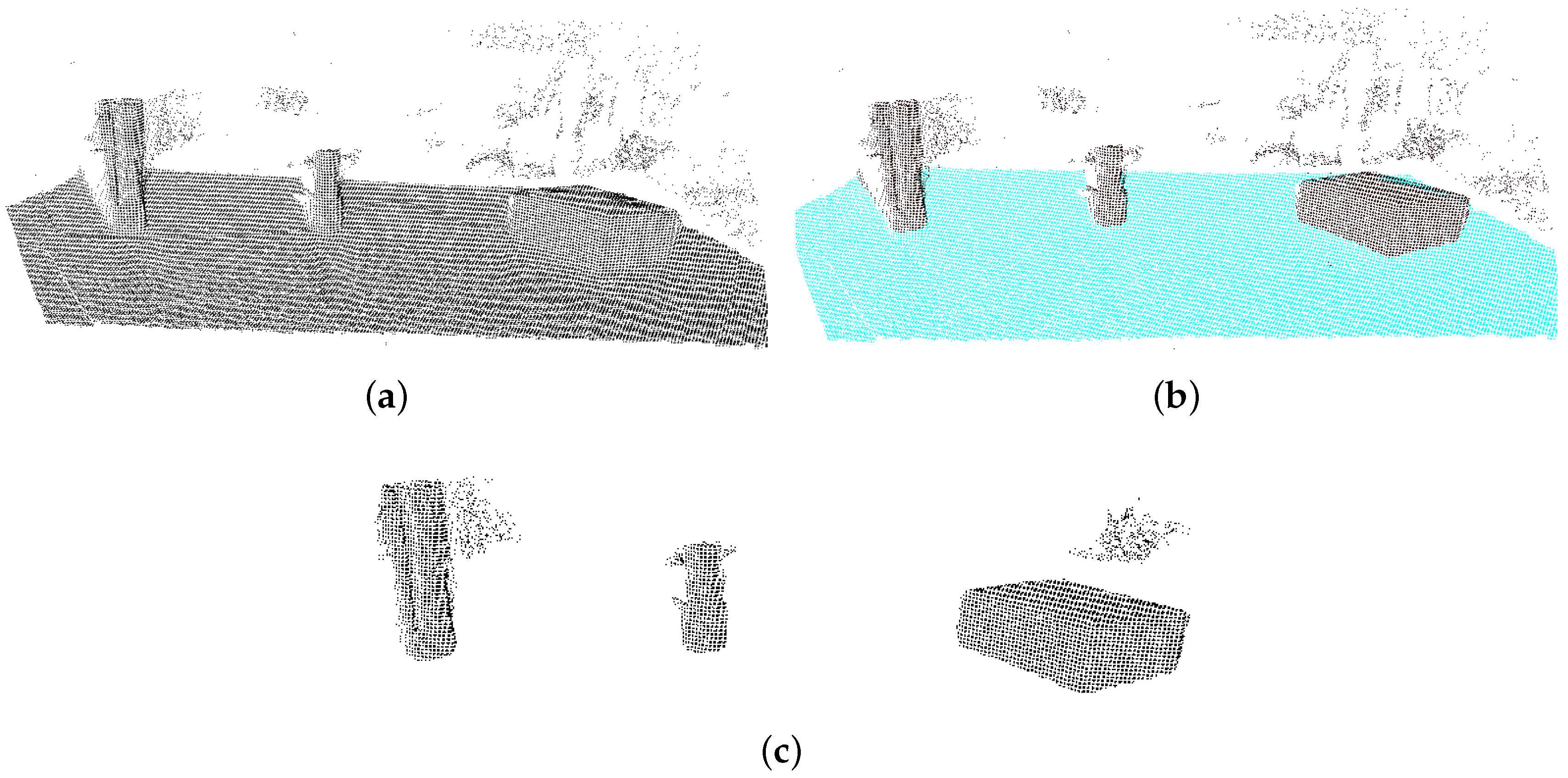
Figure 1.
The RANSAC method performed on a table with objects. (a) A scene with multiple objects placed on a table; (b) the table surface is detected using RANSAC. The cyan points are inliers of the plane estimate; (c) The scene after removing the inliers, resulting in only the points representing the three objects.
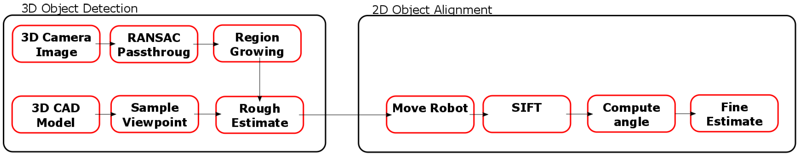
Figure 2.
Overview of the flow of the system. It can be seen that the 3D Detection System calculates a rough position estimate given a set of CAD models, and this is fed into the 2D Alignment System, resulting in a fine position and orientation estimate.
Figure 2.
Overview of the flow of the system. It can be seen that the 3D Detection System calculates a rough position estimate given a set of CAD models, and this is fed into the 2D Alignment System, resulting in a fine position and orientation estimate.
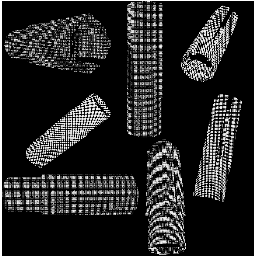
Figure 3.
Point clouds of the same object seen from different viewpoints generated from a CAD model of the object.
Figure 3.
Point clouds of the same object seen from different viewpoints generated from a CAD model of the object.
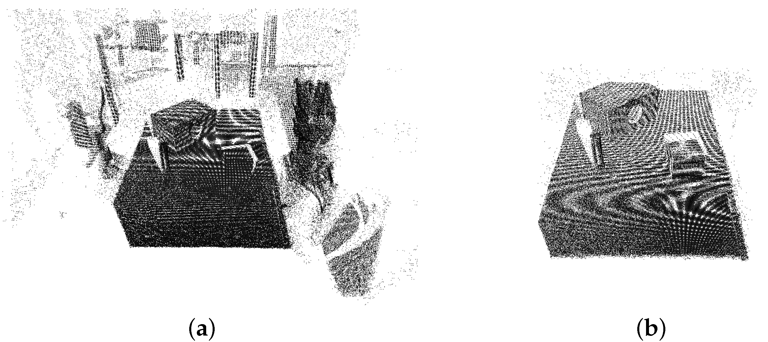
Figure 4.
Before and after pictures of removing foreground and background points. (a) Raw point cloud captured by the 3D camera; (b) Image after removing unwanted points, which are the points outside the bounds of the table.
Figure 4.
Before and after pictures of removing foreground and background points. (a) Raw point cloud captured by the 3D camera; (b) Image after removing unwanted points, which are the points outside the bounds of the table.
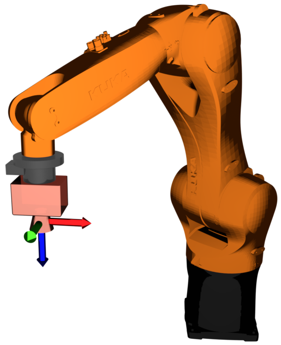
Figure 5.
Overview of the 2D camera setup. It can be seen that the camera is placed at the end-effector of the robot, and it is pointing downward.
Figure 5.
Overview of the 2D camera setup. It can be seen that the camera is placed at the end-effector of the robot, and it is pointing downward.
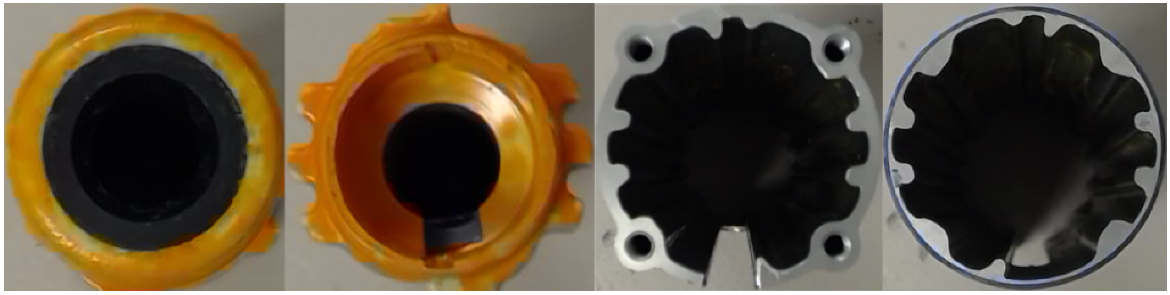
Figure 6.
Reference images for each object. From left to right: The top of object A, the bottom of object A, the top of object B, the bottom of object B.
Figure 6.
Reference images for each object. From left to right: The top of object A, the bottom of object A, the top of object B, the bottom of object B.
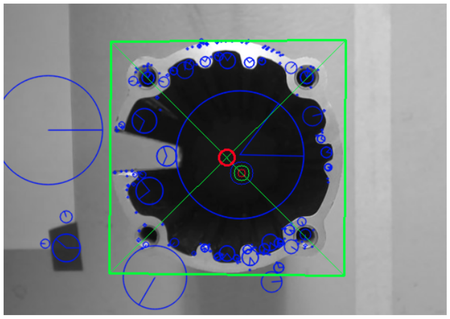
Figure 7.
The green rectangle is the position of the reference image found in the captured image. The green circle is the current rough estimate from the 3D object detection system, while the red circle is the fine estimate of the position. The blue circles are the descriptors found with the SIFT method.
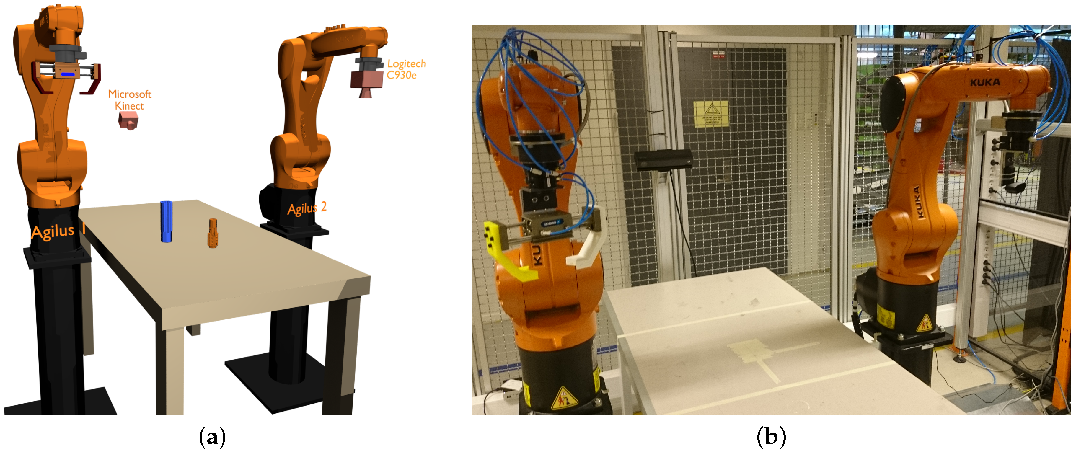
Figure 8.
Overview of the robotic cell, where the experiments were conducted. Here, there are two KUKA Agilus robots next to a table. The gripper can be viewed on the robot on the left, while the camera is on the right. Behind the table is the Microsoft Kinect One camera. (a) shows the rendered representation of the cell, while (b) shows the physical cell.
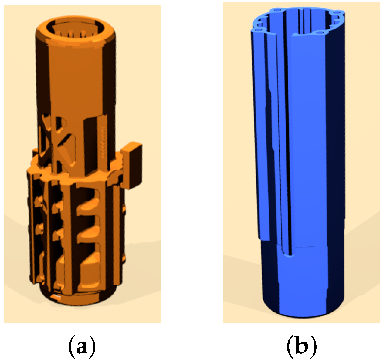
Figure 9.
The two parts used in all of the experiments. (a) Part A used in the experiment, rendered representation; (b) Part B used in the experiment, rendered representation.
Figure 9.
The two parts used in all of the experiments. (a) Part A used in the experiment, rendered representation; (b) Part B used in the experiment, rendered representation.
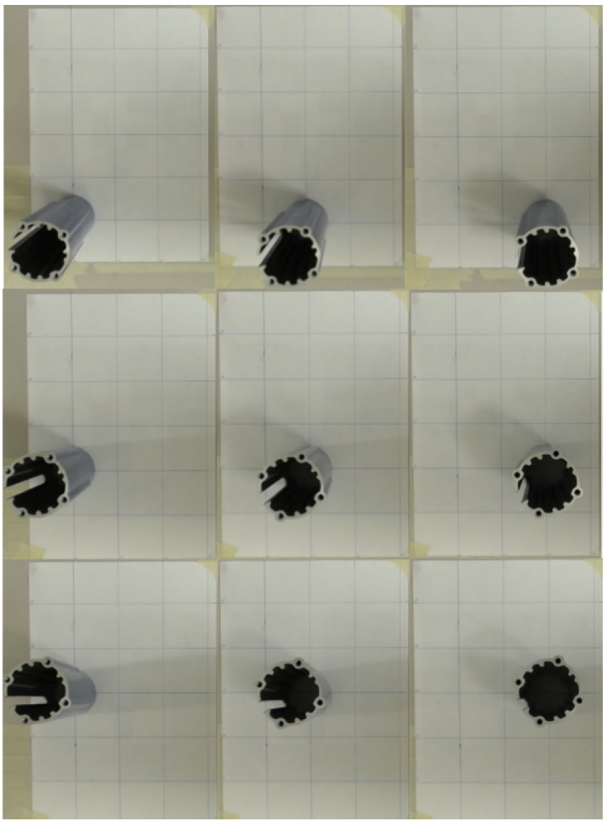
Figure 10.
Top view of the grid and the positioning of the object. Here, nine arbitrary positions of the object is seen. For each of these positions, the rough estimate of the 3D object detection system is calculated.
Figure 10.
Top view of the grid and the positioning of the object. Here, nine arbitrary positions of the object is seen. For each of these positions, the rough estimate of the 3D object detection system is calculated.
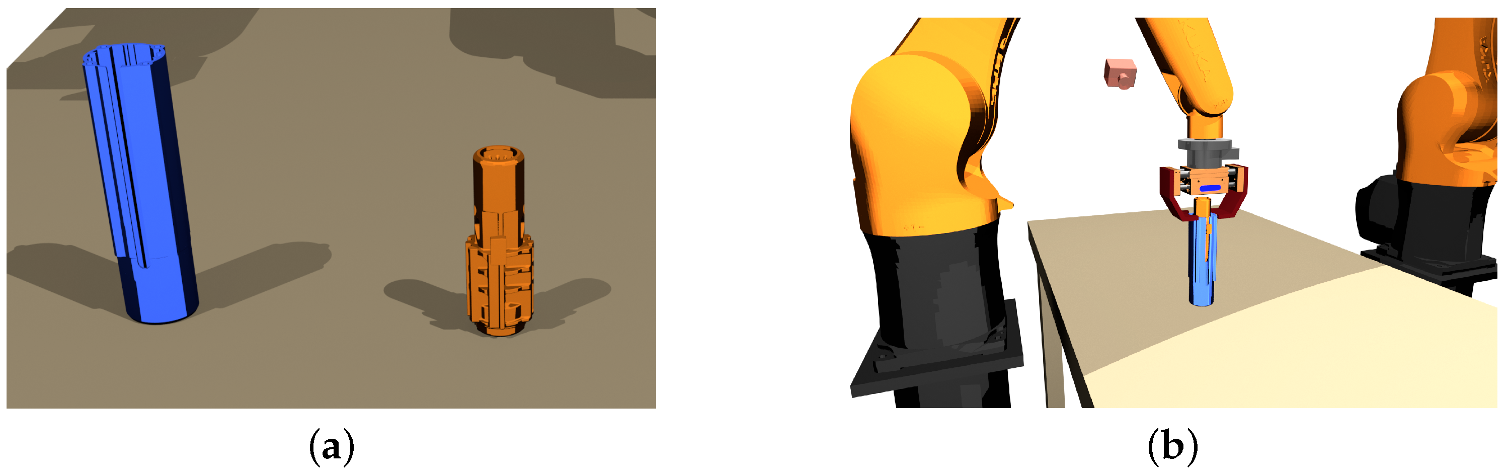
Figure 11.
Overview of the assembly operation. (a) A rendered image of the initial position of the objects; (b) A rendered image of the final position of the objects. It can be seen that the orange object should be assembled inside the blue object.
Figure 11.
Overview of the assembly operation. (a) A rendered image of the initial position of the objects; (b) A rendered image of the final position of the objects. It can be seen that the orange object should be assembled inside the blue object.
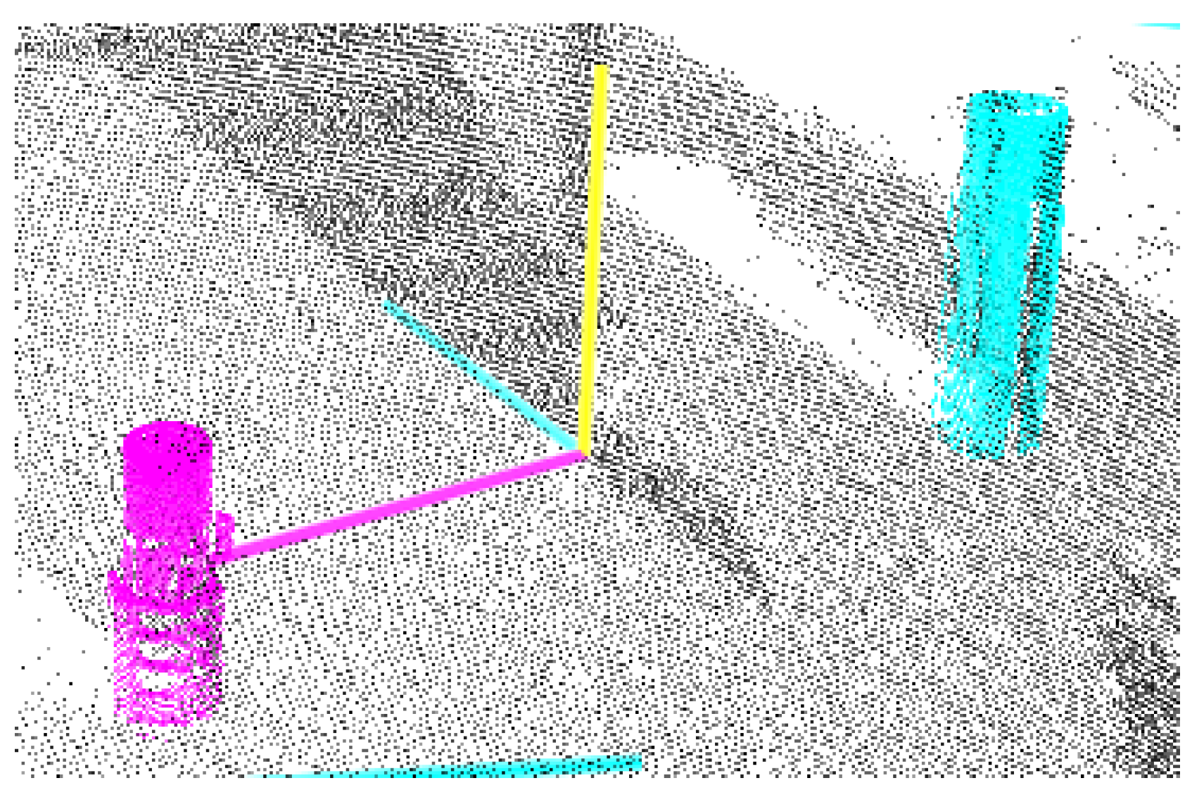
Figure 12.
Results from the 3D object detection method. The method successfully classifies each object, and determines a rough estimate of their position.
Figure 12.
Results from the 3D object detection method. The method successfully classifies each object, and determines a rough estimate of their position.
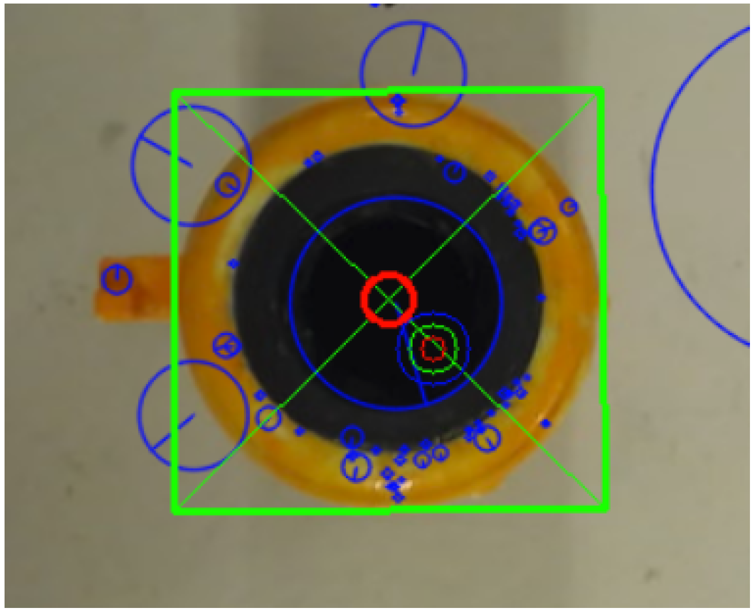
Figure 13.
The small, green circle is the position determined by the 3D object detection. Using this estimate, the method can successfully detect a fine-tuned position using the 2D camera (red circle). The error here is 5.2 mm.
Figure 13.
The small, green circle is the position determined by the 3D object detection. Using this estimate, the method can successfully detect a fine-tuned position using the 2D camera (red circle). The error here is 5.2 mm.
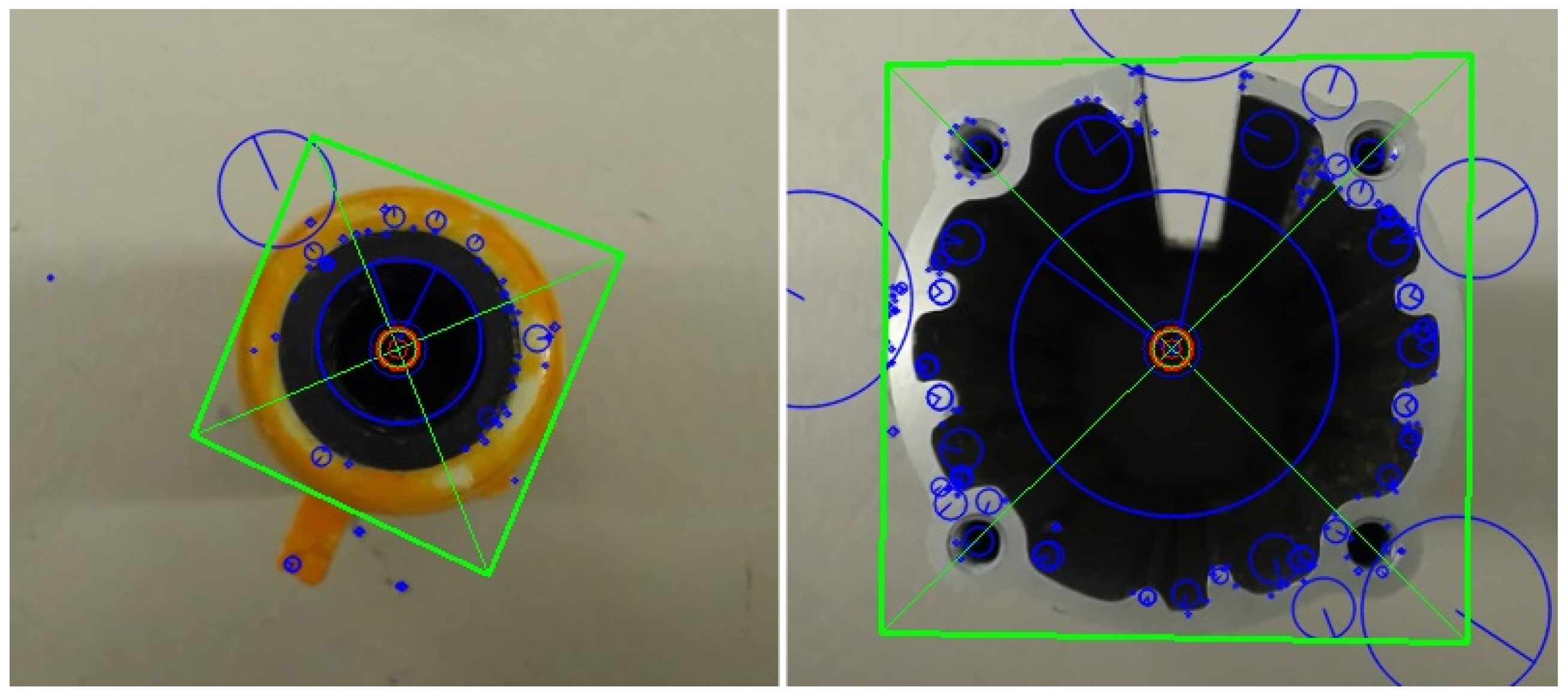
Figure 14.
SIFT used on both objects to determine their position and orientation.
Figure 14.
SIFT used on both objects to determine their position and orientation.
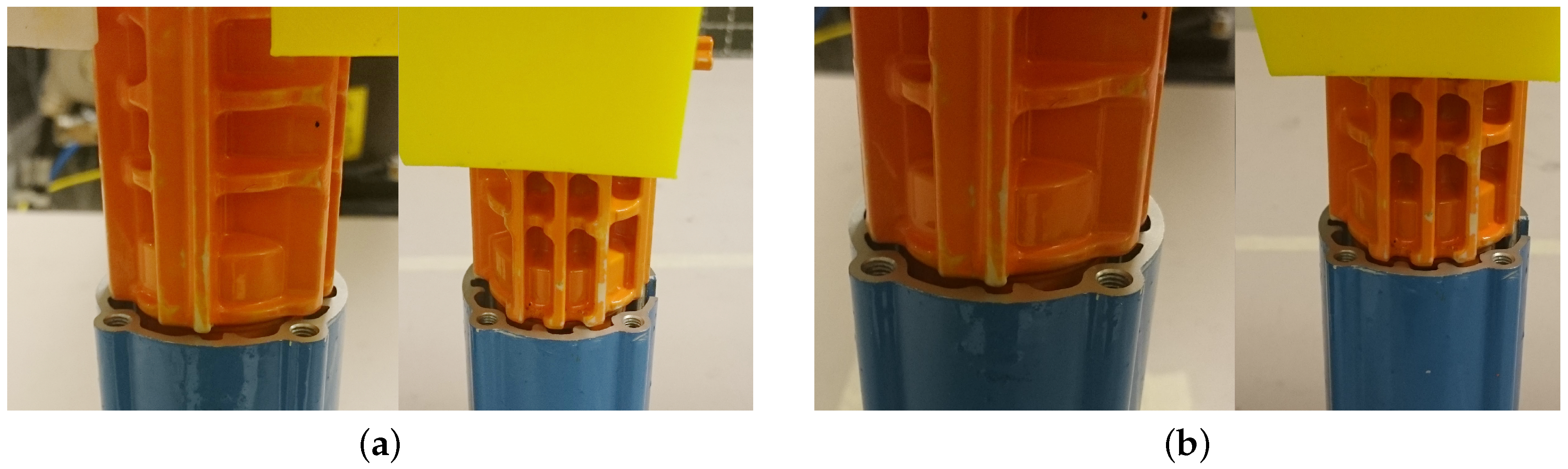
Figure 15.
Depiction of the fail and success conditions. (a) A slight deviation in the angle and position is considered a failure; (b) The position and angle are considered to be correct.
Figure 15.
Depiction of the fail and success conditions. (a) A slight deviation in the angle and position is considered a failure; (b) The position and angle are considered to be correct.
Table 1.
Minimum and maximum deviation between the true position and the estimated position of Object A. The results are based on 25 different estimates.
Table 1.
Minimum and maximum deviation between the true position and the estimated position of Object A. The results are based on 25 different estimates.
| Min/Max Recorded Values |
|---|
| Max [cm] | 1.46 |
| Max [cm] | 1.56 |
| Min [cm] | 0.43 |
| Min [cm] | 0.08 |
Table 2.
Accuracy of detecting Object A (measured in cm). The table shows the true position of Object A, the resulting estimate from the 3D object detection system, and the difference between the two.
Table 2.
Accuracy of detecting Object A (measured in cm). The table shows the true position of Object A, the resulting estimate from the 3D object detection system, and the difference between the two.
| Actual | Measured | Absolute |
|---|
| X | Y | X | Y | | |
| −5 | 5 | −6.18 | 5.4 | 1.18 | 0.4 |
| −5 | 10 | −6.25 | 10.55 | 1.25 | 0.55 |
| −5 | 15 | −6.28 | 16.11 | 1.28 | 1.11 |
| −5 | 20 | −5.17 | 21.56 | 1.28 | 1.56 |
| −10 | 5 | −11.12 | 5.08 | 1.12 | 0.08 |
| −10 | 10 | −10.83 | 10.43 | 0.83 | 0.43 |
| −10 | 15 | −10.98 | 15.92 | 0.98 | 0.92 |
| −10 | 20 | −11.46 | 20.85 | 1.46 | 0.85 |
| −15 | 5 | −15.89 | 5.2 | 0.89 | 0.2 |
| −15 | 10 | −15.81 | 10.56 | 0.81 | 0.56 |
| −15 | 15 | −15.97 | 15.77 | 0.97 | 0.77 |
| −15 | 20 | −16.18 | 21.01 | 1.18 | 1.01 |
| −20 | 5 | −20.43 | 5.4 | 0.43 | 0.4 |
| −20 | 10 | −20.68 | 10.72 | 0.68 | 0.72 |
| −20 | 15 | −20.72 | 16.27 | 0.72 | 1.27 |
| −20 | 20 | −21.18 | 21.38 | 1.18 | 1.38 |
Table 3.
Minimum and maximum deviation between the true position and the estimated position of Object B. The results are based on 25 different estimates.
Table 3.
Minimum and maximum deviation between the true position and the estimated position of Object B. The results are based on 25 different estimates.
| Min/Max Recorded Values |
|---|
| Max [cm] | 1.43 |
| Max [cm] | 1.96 |
| Min [cm] | 0.1 |
| Min [cm] | 0.06 |
Table 4.
Accuracy of detecting Object B (measured in cm). The table shows the true position of Object B, the resulting estimate from the 3D object detection system, and the difference between the two.
Table 4.
Accuracy of detecting Object B (measured in cm). The table shows the true position of Object B, the resulting estimate from the 3D object detection system, and the difference between the two.
| Actual | Measured | Absolute |
|---|
| X | Y | X | Y | | |
| −5 | 5 | −5.76 | 5.16 | 0.76 | 0.16 |
| −5 | 10 | −6.12 | 10.8 | 1.12 | 0.8 |
| −5 | 15 | −5.98 | 15.94 | 0.98 | 0.94 |
| −5 | 20 | −6.17 | 20.88 | 1.17 | 0.88 |
| −10 | 5 | −10.65 | 5.47 | 0.65 | 0.47 |
| −10 | 10 | −10.62 | 10.21 | 0.62 | 0.21 |
| −10 | 15 | −10.73 | 15.81 | 0.73 | 0.81 |
| −10 | 20 | −10.91 | 20.79 | 0.91 | 0.79 |
| −15 | 5 | −15.22 | 5.46 | 0.22 | 0.46 |
| −15 | 10 | −15.46 | 10.62 | 0.46 | 0.62 |
| −15 | 15 | −15.71 | 16.2 | 0.71 | 1.2 |
| −15 | 20 | −15.85 | 21.14 | 0.85 | 1.14 |
| −20 | 5 | −20.1 | 5.43 | 0.1 | 0.43 |
| −20 | 10 | −20.73 | 10.06 | 0.73 | 0.06 |
| −20 | 15 | −20.26 | 16.35 | 0.26 | 1.35 |
| −20 | 20 | −21.43 | 21.96 | 1.43 | 1.96 |
Table 5.
The difference between the maximum and minimum measured orientations for Object A. The first table is the deviation between the maximum and minimum angle when the object is positioned at 0°, both with using SIFT and with a SIFT/SURF hybrid. The second table is when the object is positioned at 90°. The measurements are given in degrees.
| 0 Degrees | −90 Degrees |
|---|
| SIFT | SIFT/SURF | SIFT | SIFT/SURF |
| 1.7469 | 5.4994 | 1.1102 | 7.9095 |
Table 6.
The difference between the maximum and minimum measured orientations for Object B. The first table is the deviation between the maximum and minimum angle when the object is positioned at 0°, both with using SIFT, and with a SIFT/SURF hybrid. The second table is when the object is positioned at 90°. The measurements are given in degrees.
| 0 Ddegree | −90 Degrees |
|---|
| SIFT | SURF | SIFT | SURF |
| 0.07888 | 0.2041 | 0.1721 | 0.1379 |


