Motion Planning for a Chain of Mobile Robots Using A* and Potential Field

Abstract

Traditionally, motion planning involved navigating one robot from source to goal for accomplishing a task. Now, tasks mostly require movement of a team of robots to the goal site, requiring a chain of robots to reach the desired goal. While numerous efforts are made in the literature for solving the problems of motion planning of a single robot and collective robot navigation in isolation, this paper fuses the two paradigms to let a chain of robot navigate. Further, this paper uses SLAM to first make a static map using a high-end robot, over which the physical low-sensing robots run. Deliberative Planning uses A* algorithm to plan the path. Reactive planning uses the Potential Field Approach to avoid obstacles and stay as close to the initial path planned as possible. These two algorithms are then merged to provide an algorithm that allows the robot to reach its goal via the shortest path possible while avoiding obstacles. The algorithm is further extended to multiple robots so that one robot is followed by the next robot and so on, thus forming a chain. In order to maintain the robots in a chain form, the Elastic Strip model is used. The algorithm proposed successfully executes the above stated when tested on Amigobot robots in an office environment using a map made by the Pioneer LX robot. The proposed algorithm works well for moving a group of robots in a chain in a mapped environment.

1. Introduction

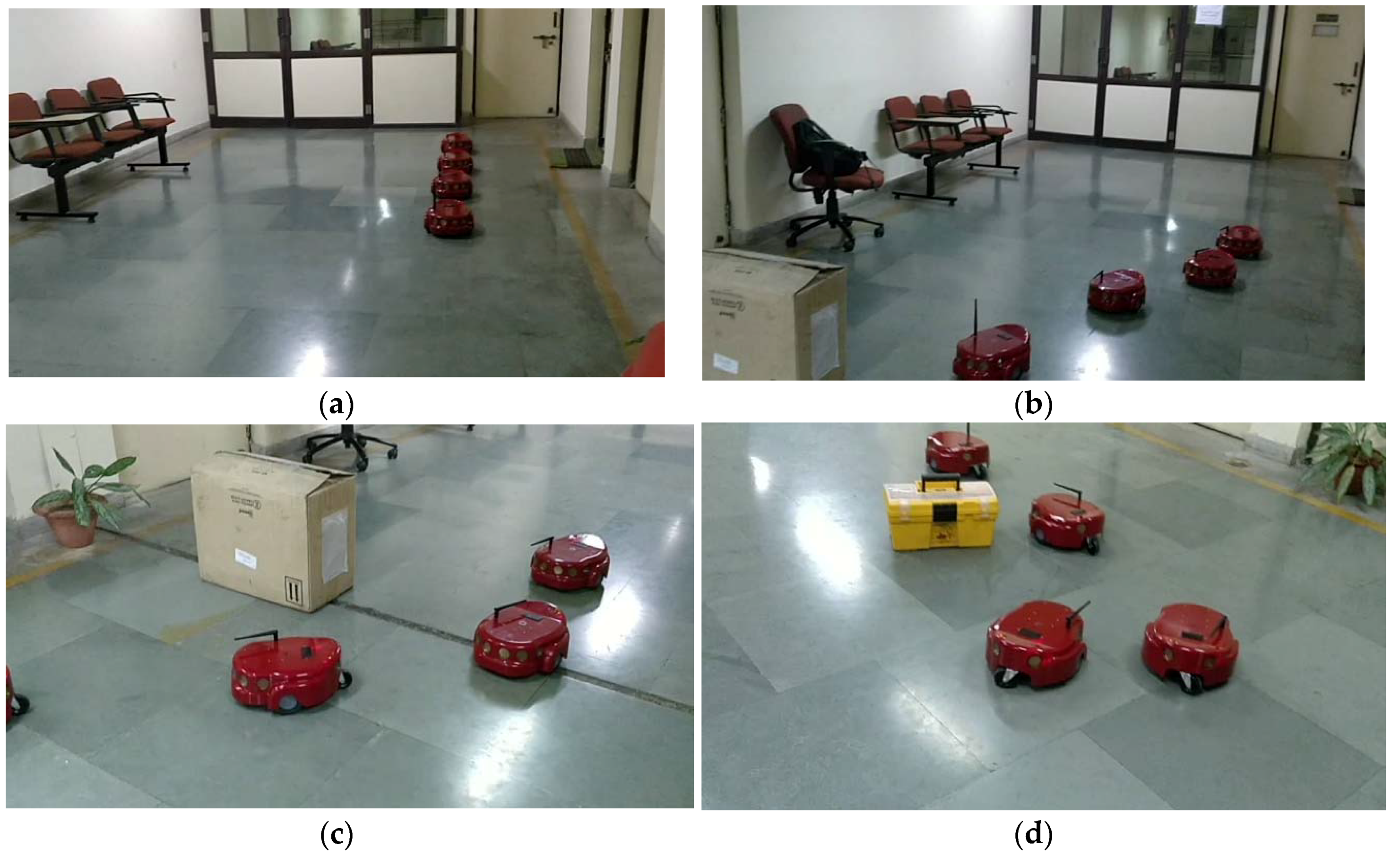
Chaining of mobile robots is very useful as it leads to minimization of costs or better chances of success than that of deploying a single robot. Interest in the field of multiple robots coordinating with each other is increasing as they have many applications in areas such as collaborative exploration of mapped or unmapped areas, automated highway or flight systems, surveillance, and search and rescue missions. In this paper, we address the problem of moving a team of mobile robots from an initial state to a final state along the shortest possible path while also avoiding obstacles on its way. A chain is used as a structuring element for the team with the inspiration of a chain of school kids going to a zoo, a chain of workers going to a factory, etc. A chain is the most elegant structure scalable to a very large level while allowing easy passage of the other people, especially in a robotic context. Using a grid or circular arrangement of robots would create a mob that is hard to surpass by others when the number of robots are very large. The practical applications of chaining in a robotic context include using multiple mobile robots to transfer goods in a warehouse or shopping mall, using multiple robots to carry out repairs that require collective effort of multiple robots in which context they can navigate as a chain, etc. Th formation of a straight line of robots has its applications in various scenarios as well. For example, using this algorithm, trains can be built, which can cross each other, if required, and still stay on their own course, together, and in a linear fashion. This will prevent the need of rerouting the trains and the need to design routes in such a way that two trains crossing each other do not meet at the same time. This will save effort, time, and resources.

In this paper, an efficient multi-robot path planning approach is proposed for moving the robots in a chain-like fashion where one robot is followed by the next and the next robot is followed by the robot after that. The robots take the shortest path possible from their source to their goal. The path planning for the master robot is done in two steps:

• Deliberative Planning—A path is found from source to goal over a static map. This data is computed before running the robot. The technique is optimal and complete but is computationally expensive and cannot be done on the fly.
• Reactive Planning—The immediately next move is computed based on obstacles around the goal. This planning is done during run-time. The technique is neither optimal nor complete but is real-time in nature and therefore ideal for moving obstacles, new obstacles, and to counter large errors in localization or control.

A hybrid of deliberative and reactive planning makes a powerful algorithm, in which case the reactive planning tries to achieve a sub-goal given by the deliberative planning. When dealing with a chain of mobile robots, we need both deliberative planning and reactive control so that path planning involves reaching of robots to goal configuration taking the shortest path avoiding static obstacles in the map. Reactive control allows us to deal with dynamic obstacles over our static map while executing the global planned path.

Furthermore, the aim is to keep robots in a straight chain as much as possible. For this purpose, ‘Elastic Strip approach’ is used, whereby an elastic strip is assumed to exist between the first and the last robot’s positions and other robots try to stay as close as possible to the elastic strip.

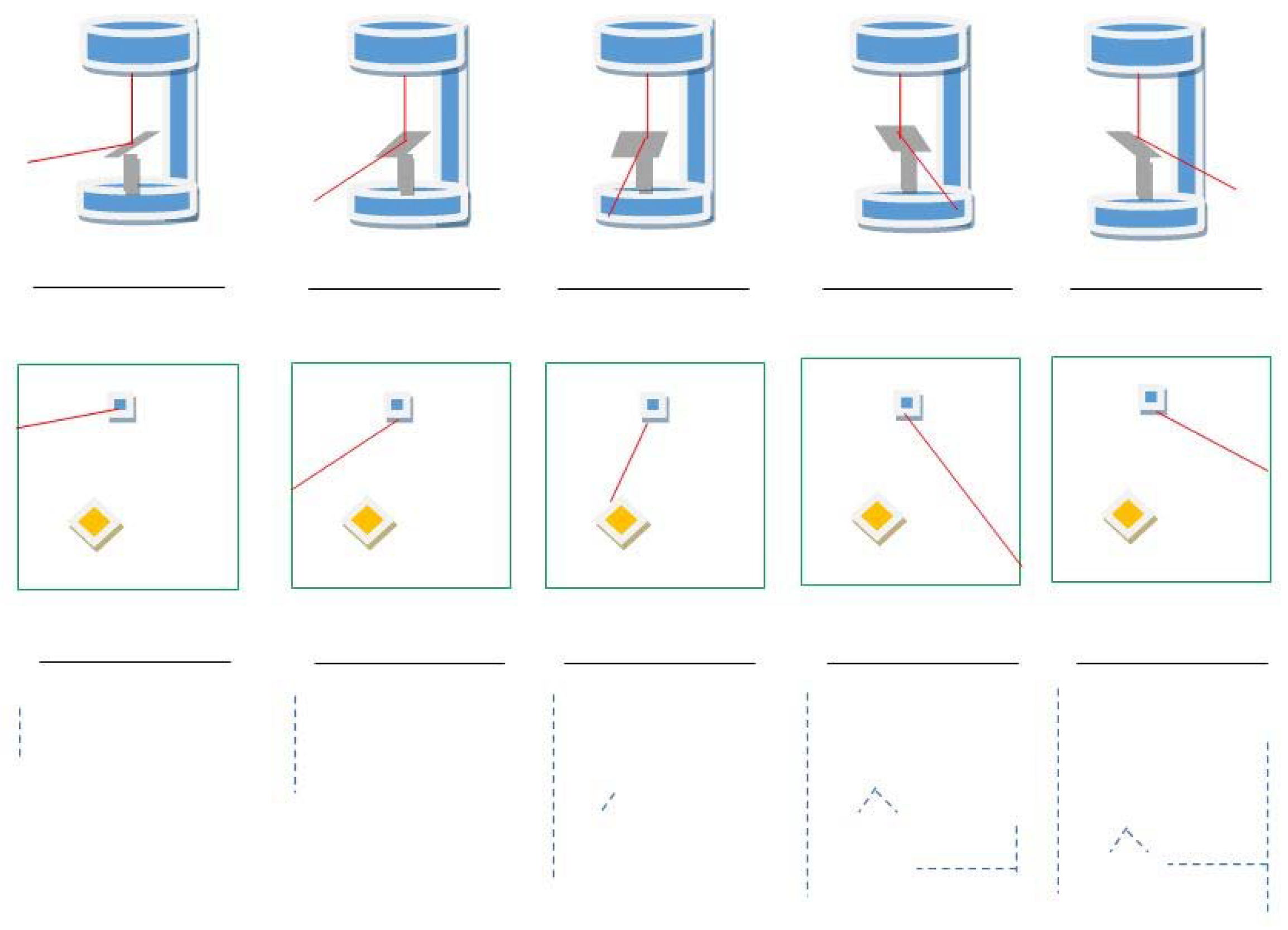
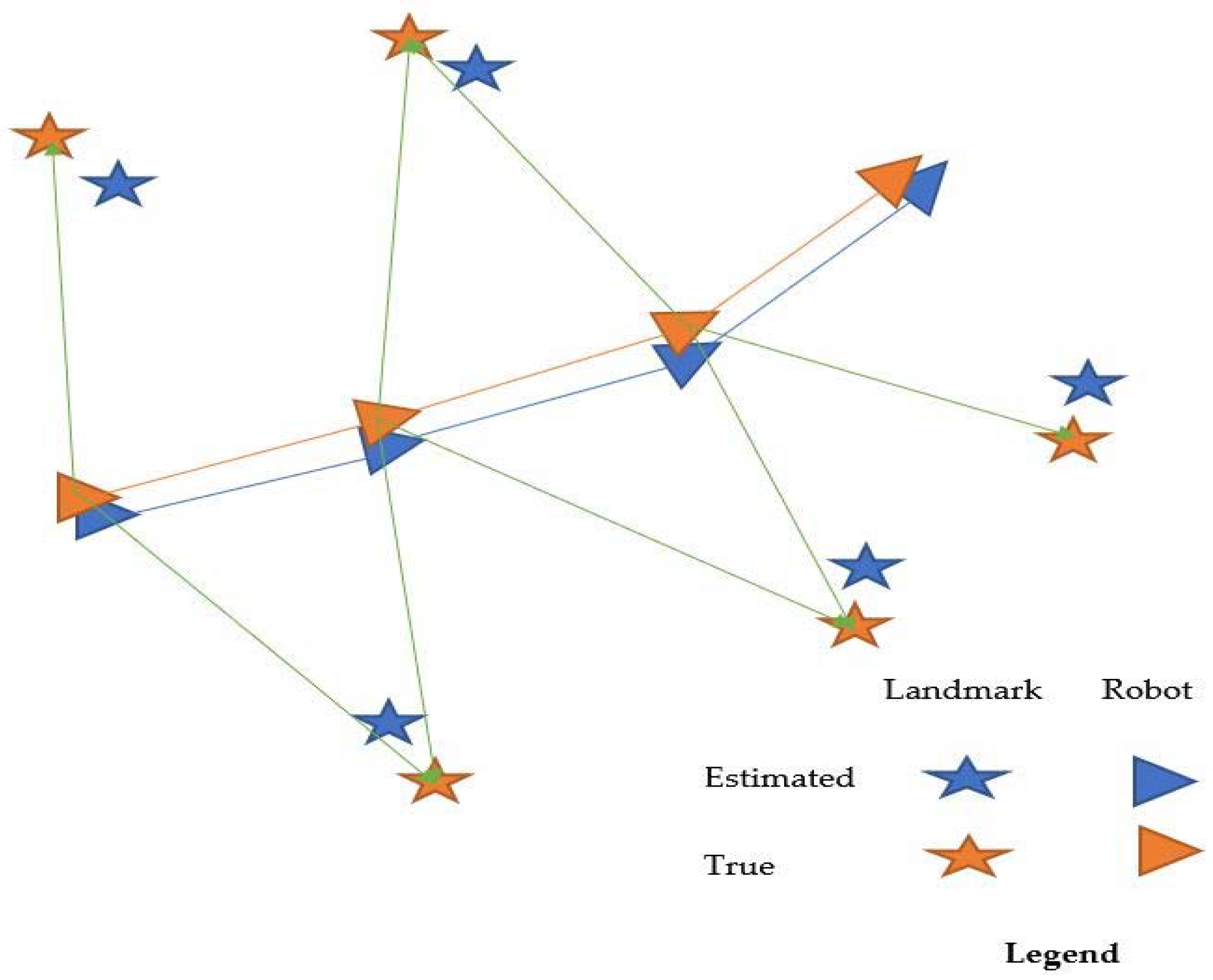
The first step in the process is creating a static map. This is done using a technique called Simultaneous Localisation and Planning (SLAM) [1]. In robotics, the sensors make a local map with respect to the robot’s position, and hence integration with global map cannot happen without knowing the robot’s position while the vision sensors try to estimate the position of the robot based on a priori known map. Since the location is computed using a map and vice versa, SLAM tries to solve both problems simultaneously. A LIDAR sensor is used to compute the distance between the robot, creating the map and the obstacles/features found in the map. The robot has encoders on wheels to give indication of the distance moved. Filtering algorithms are used to guess the position based on a motion model and sensor readings. Once all the features are mapped to the direction and position of the robot, a map is created.

In the literature, a lot of effort is given toward the motion planning of a single robot from a source to a pre-known goal, for which a variety of methods have already been implemented for dynamic environments. Similarly, a lot of effort has been made for flocking and collective motion of robots. The typical displayed behaviours include a straight line motion of a swarm of robots amidst obstacles. This paper solves the two problems simultaneously. The problem is challenging from the perspective of a single robots, as the multiple robots affect each other’s behaviours and thus make it difficult for any single robot to move. From the perspective of collective robot navigation, the problem is more challenging, since the path being followed by collective robots will go through a lot of turns, narrow areas, and areas requiring fine manoeuvres. Further, very few approaches actually make a map of the real environment using SLAM techniques to test the approach on real robots. Simulations are not always indicative of the real sensing and actuation uncertainties. The approach fist uses Pioneer LX robot to create a map. Then, the approach uses multiple Amigobot robots to collectively move in a chained mechanism in the map.

Deliberative path planning in this paper is done using A* algorithm [2]. This algorithm takes into account the heuristic for shortest path planning. The heuristic for any given point gives the general idea of the final distance from that point to the goal. The point in the neighbourhood of the current point is selected in such a way that it has the minimum expected distance to the goal. The heuristic used should be such that it is admissible and consistent. The heuristic being admissible means that the final shortest distance possible to the goal should always be greater than or equal to the value given by the heuristic. The heuristic being consistent means that the distance from a given point to the goal should always be less than or equal to the sum of distance between that point and some intermediate point and goal and the same intermediate point. We use the Euclidean distance between two points as the heuristic value.

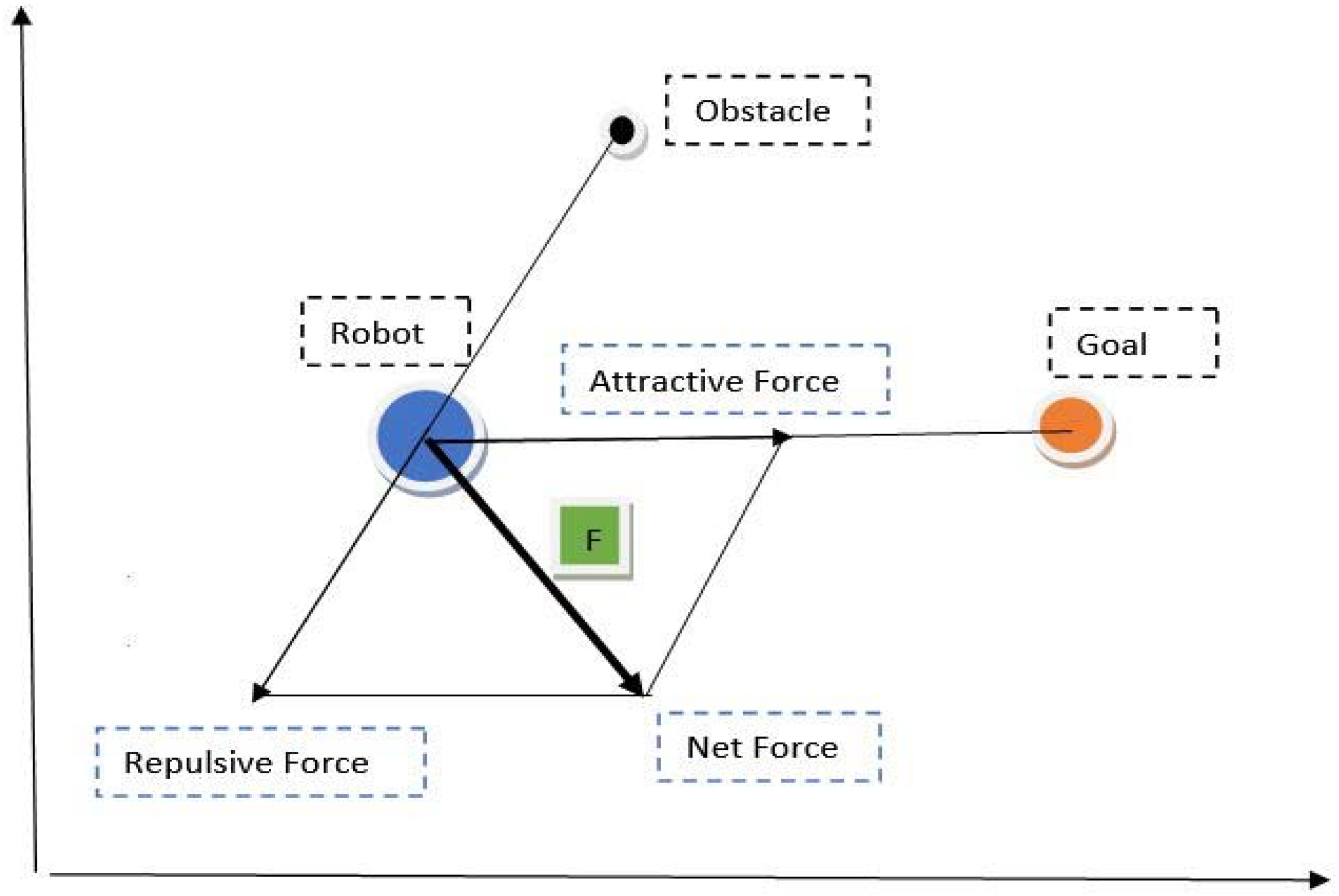
The Potential Field [3] approach uses the same properties as those of the electrostatic potential, wherein the objects of same charge repel each other and the objects of opposite charges attract each other. The goal is hence given a positive charge, and the robots and obstacles are given the same negative charge. The goal attracts the robot, while the obstacles repel the robot. This divides the whole terrain into a series of potential highs and lows, successfully suggesting a path of potential laws for the robot to follow.

The chain of robots more often does not maintain a straight line. In order to keep the robots in a straight line, the elastic strip model is used, whereby an elastic strip is assumed to exist between the first and the last robot. The intermediate robots act as pegs stretching the elastic strip, thus creating tension. Due to this tension, a force that is directly proportional to the distance of the robot from the elastic strip is exerted on the robots in the direction of the elastic strip. This effectively causes the robots to align themselves in a linear fashion.

The two approaches can effectively be merged to form a better and efficient path planning algorithm. Also, the same algorithm can be applied on a set of robots in a master–slave fashion, wherein the master robot leads the slave robot and the slave robot follows the master robot while avoiding obstacles on its own. We have used this approach so as to allow a chain of robots to reach the goal state. The elastic strip model helps these robots to stay in a linear formation, even during motion.

2. Literature Survey

A lot of work exists to move robots from a source to a goal. Sariff and Buniyamin [4] explained the various approaches and problems related to robot path planning and navigation. They compare the various algorithms for robot path planning, such as the A* algorithm, potential field based algorithms, and genetic algorithms. They also discuss the strengths and weaknesses of each of the above algorithms. Ratering and Gini [5] proposed the use of hybrid potential field for robot navigation in a known map with unknown moving obstacles. They use a global potential field that includes the static information of the map where the global minimum state is the global. The local potential field is limited to the area near the robot, and its primary purpose is to push the robot away from the obstacles in its path. The local potential field is calculated with the help of sonar sensors present on the robot. The global potential field is computed only once initially, whereas the local potential field is computed continuously. The paper also presented results of simulation with up to 50 moving objects. Kala et al. [6] solved the problem of navigation of a single robot using a hybrid and fuzzy logic and A* algorithm. The algorithm parameter could be tweaked to get more reactive or more deliberative behaviour.

Hart, Nilsson, and Raphael [7] addressed the problem of finding the minimum cost in a graph using various heuristic strategies that are admissible and consistent. The paper also showed the optimality of their approach. Parsediya, Agarwal, and Guruji [8] explained how the traditional A* algorithm is time-consuming, as the environment is continuously changing, and the rules must be updated to compute a collision free path leading to higher processing times. Thus, they proposed a modification where they determined the heuristic value just before collision rather than initially thus decreasing the processing time. The simulation of the paper showed good decrement in the processing time of the algorithm versus the original algorithm. Warren [9] explained path planning techniques used for robot manipulators and mobile robots using artificial potential fields. Potential fields are used because they allow users to plan a path relatively quickly and effectively without collisions with obstacles. The method used uses a trial path that is modified with the help of potential fields to devise the final path. This method takes care of the local minima problem associated with potential fields.

Hess et al. [10] explained the creation of floor maps using the SLAM technique with the help of portable laser range-finders known as LIDARs. Loop enclosures are computed using scan to sub map matching. The resulting maps are of high quality and accuracy due to the precision of the LIDARs. Kavralu et al. [11] discussed a motion planning approach for mobile robots in static environments. First, probabilistic roadmaps were created during the learning phase of collision free paths and stored as a graph where nodes corresponded to the vertices. During the query phase, the user gave the start and goal configurations of the roadmap, and after that, the graph was searched for the path between the start and goal configurations.

Abatari and Tafti [12] explained the creation of a path following controller for a mobile robot using a fuzzy PID controller wherein fuzzy logic is used for tuning of the parameters of the PID controller. The controller thus built is tested on a simulation model of a car and results in better performance than a standard PID controller. Chong and Kleeman [13] described the process of map building in an indoor environment with the help of sonar sensor arrays and where the odometry information is obtained from the wheel encoders. External features identified by the sonar such as walls were also used by the odometry module as supplementary information to minimize the errors accumulated in the encoder readings. Individual sonar readings were incrementally merged into the main map configuration to produce better and more realistic results such as a wall may be seen by the robot as a set of closely located collinear planar elements that is merged by the map update algorithm in order to produce better and precise results.

Burgard et al. [14] explained the problem of mapping an unknown environment by a team of robots while minimizing the exploration time. It presents a probabilistic approach to assigning points in the environment to robots based on the cost of reaching the target point and upon the size of the unexplored areas the sensors can cover. The paper also presents its results on simulation and real-time runs. Pati and Kala [15] made a small mobile robot called a slave that follows a bigger mobile robot called a master. The master robot was remotely operated. Desai, Ostrowski, and Kumar [16] explained using feedback laws on how to move a group of robots in a formation that use only local sensor information in a leader–follower motion. They used distance and orientation information of the robots in order to maintain the formation. The paper also presented simulation results to control six robots moving around an obstacle.

Chen and Zohu [17] explained the problem of defining a path planning algorithm using the Quantum Genetic Algorithm. The solution works effectively for space based manipulators and help astronauts to avoid the harsh conditions faced when in space. As the manipulators are space-based, the motion of the manipulators also depends on the path taken by the joints. The joint trajectories are parameterised using sinusoidal functions, and other parameters are determined.

Hamaguchi and Taniguchi [18] explained in their paper how the obstacle avoidance algorithms vary if the degrees of freedom changes. They focus their work on robots having seven degrees of freedom (DOG). The seven DOF manipulators have kinematic redundancy that must be taken care of. Impedance control is suggested as the method to avoid obstacles in this paper.

K. Chang, J. Hwan, E. Lee, and S. Kazadi [19] describe the swarm engineering technique to create swarm mediated systems. This is further used to develop a multi-chain robot system. The benefits of using this are also shown.

Sebastian Abshoff, Andreas Cord-Landwehr, Matthias Fischer, Daniel Jung, and Friedhelm Meyer auf der Heide [20] consider the problem of gathering of swarm of robots. Initially, the robots form a chain with a connectivity, and they maintain this till the end. The chains are then shorted until all the robots are located inside a 2x2 grid. The method suggested is completely local in nature. Each robot can only see its neighbours. Thus, the robots do not have any knowledge of the global progress of the system. The algorithm needs linear time.

Christopher James Shackleton, Rahul Kala, and Kevin Warwick [21] have discussed the investigation of the problem of generating a collision free trajectory for assisting drivers. The current state of the vehicle is determined in order to do so. The vehicles communicate with each other regarding the environment. Repulsive potential is applied on the vehicles from the ones near it in order to maintain a tradeoff between the optimum path and obstacle avoidance.

Steven Recoskie, Eric Lanteigne and Wail Gueaieb [22] have discussed the comparative study of various factors in planning the trajectory of unmanned airships. The planner tries to optimise the trajectory in terms of time, energy consumption and collision avoidance.

The literature suggests that, while a lot of work is done for motion planning of a single robot and collective motion of multiple robots, there is slim work on the two problems simultaneously. Further, most results are on simulations or synthetic maps. There is slim work on integrating the problem with map building of a real office environment and using the same for the planning.

3. Background

3.1. Sensing

LIDAR is a surveying method used in making maps, and in the fields of archaeology, seismology, physics etc. The way we use LIDAR in map making is to find distances to objects in an environment with the help of illuminating them with pulsating laser lights and then measuring the pulses with a sensor. After that, we can find the distance to the target as we already know the time after which the pulsed laser light was received and the wavelength of the laser used. Figure 1 discusses the working of a LIDAR.

SONAR is another type of sensor. Traditionally, sonar [23] has been used in military and marine applications or for the use of medical imaging. However, ultrasonic range transducers have become popular in the field of mobile robotics due to their simplicity and low cost. Sonar works by emitting a sound wave and waiting for it to bounce back. The robot measures the distance based on the time taken between receiving and emitting as we already know the wavelength of sound. Sonar data is usually noisy, and we cannot rely on a single sonar. Thus, we use a sonar sensor array in a robot for better coverage and accuracy.

3.2. SLAM

In robot mapping and navigation, SLAM is the problem of finding the location of a robot in an unknown environment and also simultaneously creating or updating the map of the environment. SLAM is usually performed with the help of topological maps, wherein the robot stores its location as graph nodes and then annotating the graph. In order to perform SLAM, various sensors are used such as vision-based, 2-D or 3-D LIDAR–based, 2-D or 3-D sonar sensors, cameras (stereo, RGBD, and monocular), radar, and Wi-Fi. Dynamic environments pose a challenge to SLAM as the map keeps on changing. In this paper, we would be using LIDAR based SLAM to map the environment. Figure 2 demonstrates the working of SLAM.

3.3. Reactive Planning

The Artificial Potential Field approach is used by the robot to move toward the goal. The configuration is such that the goal is positively or negatively charged, and the robot is oppositely charged. Thus, there is a potential field and the robot moves along the gradient. One scenario can be that the goal is positively charged and the robot is negatively charged

As the gradient decreases when the robot moves toward the goal, so it will move to minimize this gradient. So, we can say that the goal always pulls the robot toward itself. Now there are obstacles in the path that the robot should not collide with. The artificial potential concept provides an elegant solution to this problem. If the obstacles are having the same charge as the robot, obstacles and robots will always repel each other, thus there are no collisions. According to the above scenario, the set of obstacles would be negatively charged. The gradient can be considered forces. So, a configuration would exert force trying to minimize the energy. Thus, having the minimum energy, the robot will move to attain this configuration. The motion of the robot stops when it reaches a point of zero gradient theoretically.

The forces can be classified as attractive and repulsive. The attractive potential is given by Equation (1), while the force due to the same is given by Equation (2).

$$U_{att}\left(q\right)=\{\begin{array}{c}\frac{1}{2}\epsilon d^2\left(q, q_{goal}\right), d\left(q,q_{goal}\right)\le d_{goal}^{\ast }\\ d_{goal}^{\ast }\epsilon d\left(q,q_{goal}\right)-\frac{1}{2}\epsilon {(d_{goal}^{\ast })}^2, d\left(q,q_{goal}\right)>d_{goal}^{\ast }\end{array},$$

(1)

$$\nabla U_{att}\left(q\right)=\{\begin{array}{c}\epsilon \left(q- q_{goal}\right), d\left(q,q_{goal}\right)\le d_{goal}^{\ast }\\ \frac{d_{goa{l}^{\epsilon (q-q_{goal})}}^{\ast }}{d\left(q,q_{goal}\right)}, d\left(q,q_{goal}\right)>d_{goal}^{\ast }\end{array},$$

(2)

where,

◾

$U_{att}\left(q\right)=Potential Function for attraction$

◾

$d\left(q,q_{goal}\right)= distance between robot q and its goal$

◾

$d_{goal}^{\ast }=threshold distance separating conic and quadratic potential$

◾

$\epsilon = parameter used to scale the effect of the attractive potential$

◾

$\nabla U_{att}\left(q\right)=attractive gradient$

There are two sections between which the planner switches from conic force to quadratic force. The section at a distance greater than $d_{goal}^{\ast }$ is the conic section in which the force acting on the robot is directly proportional to the distance between robot and its goal (larger the distance, larger will be the force but linear so that robot does not cross the obstacles to reach its goal) and the section less than or equal to $d_{goal}^{\ast }$ is the quadratic section in which the force acting on the robot is directly proportional to square of the distance between the robot and the goal to let the robot reach its goal (as the distance decreases, force also decreases causing robot to stop in the way if there is an obstacle near the goal).

The repulsive potential is given by Equation (3) and the repulsive forces is given by Equation (4).

$$U_{rep}\left(q\right)=\{\begin{array}{c}\frac{1}{2}\mathsf{\eta }{\left(\frac{1}{D\left(q\right)}-\frac{1}{Q^{\ast }}\right)}^2, D\left(q\right)\le Q^{\ast }\\ 0, D\left(q\right)>Q^{\ast }\end{array},$$

(3)

$$\nabla U_{rep}\left(q\right)=\{\begin{array}{c}\mathsf{\eta }\left(\frac{1}{Q^{\ast }}-\frac{1}{D\left(q\right)}\right)\frac{1}{D^2\left(q\right)}\nabla D\left(q\right), D\left(q\right)\le Q^{\ast }\\ 0, D\left(q\right)>Q^{\ast }\end{array},$$

(4)

where,

◾

$U_{rep}\left(q\right)=Potential function for repulsion$

◾

$Q^{\ast }=distance at which robot starts ignoring obstacle$

◾

$D\left(q\right)=distance to the closest obstacle$

◾

$\mathsf{\eta }=gain on repulsive gradient$

◾

$\nabla U_{rep}\left(q\right)=repulsive gradient$

The repulsive force is inversely proportional to the distance between the robot and the obstacle. Moreover, the force only comes into the picture whenever the robot moves into the vicinity of the obstacle (i.e., the distance between the robot and the obstacle is less than or equal to $Q^{\ast }$). As the robot moves near the obstacle, the repulsive force increases thus it tries to deflect away from the obstacle more strongly. The combination of attractive and repulsive forces is responsible for the motion of the robot. Figure 3 demonstrates this.

3.4. Elastic Strip Model

This model suggests a technique to align a particular state of multiple units acting together in a fixed manner. An elastic strip is assumed to exist on the accepted values of states. These states can be the position of the units involved. The units whose states differ from the elastic strip act as pegs distorting the strip. This distortion creates tension in the elastic strip. In order to release the tension, the elastic strip exerts a force on the units directly proportional to the deviation, thus pulling the units toward itself. This helps them align in the manner desired.

4. Methodology

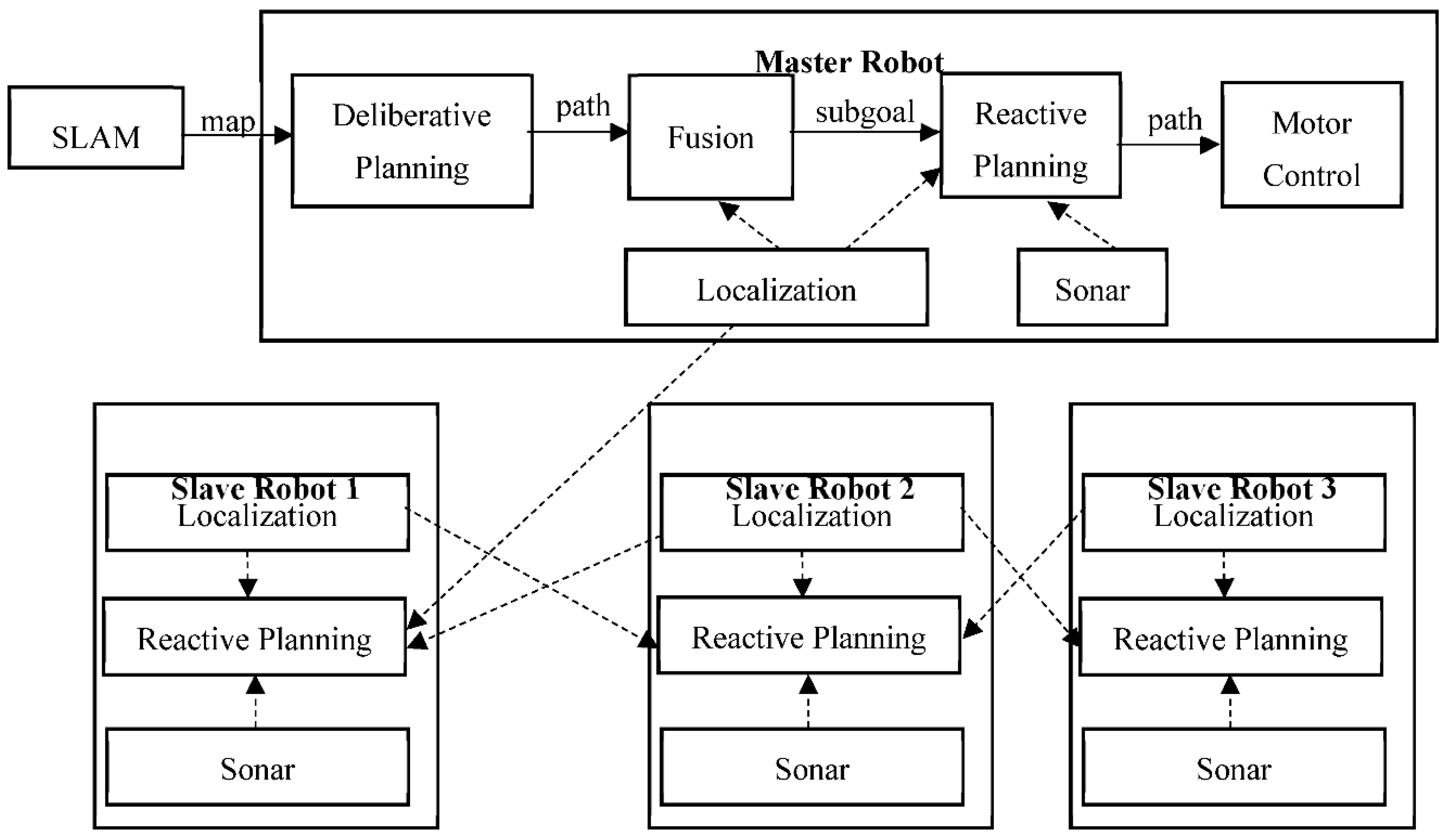
The overall methodology of the approach is shown in Figure 4. The approach needs a map that is produced by using SLAM in the absence of any dynamic obstacles. Thereafter, the master robot plans its path from source to goal. First, a deliberative path is computed, which acts as a guide for reactive control. The technique is used for the navigation of multiple robots forming a chaining behaviour. The details of all modules are presented in the following sub-sections.

4.1. Mapping

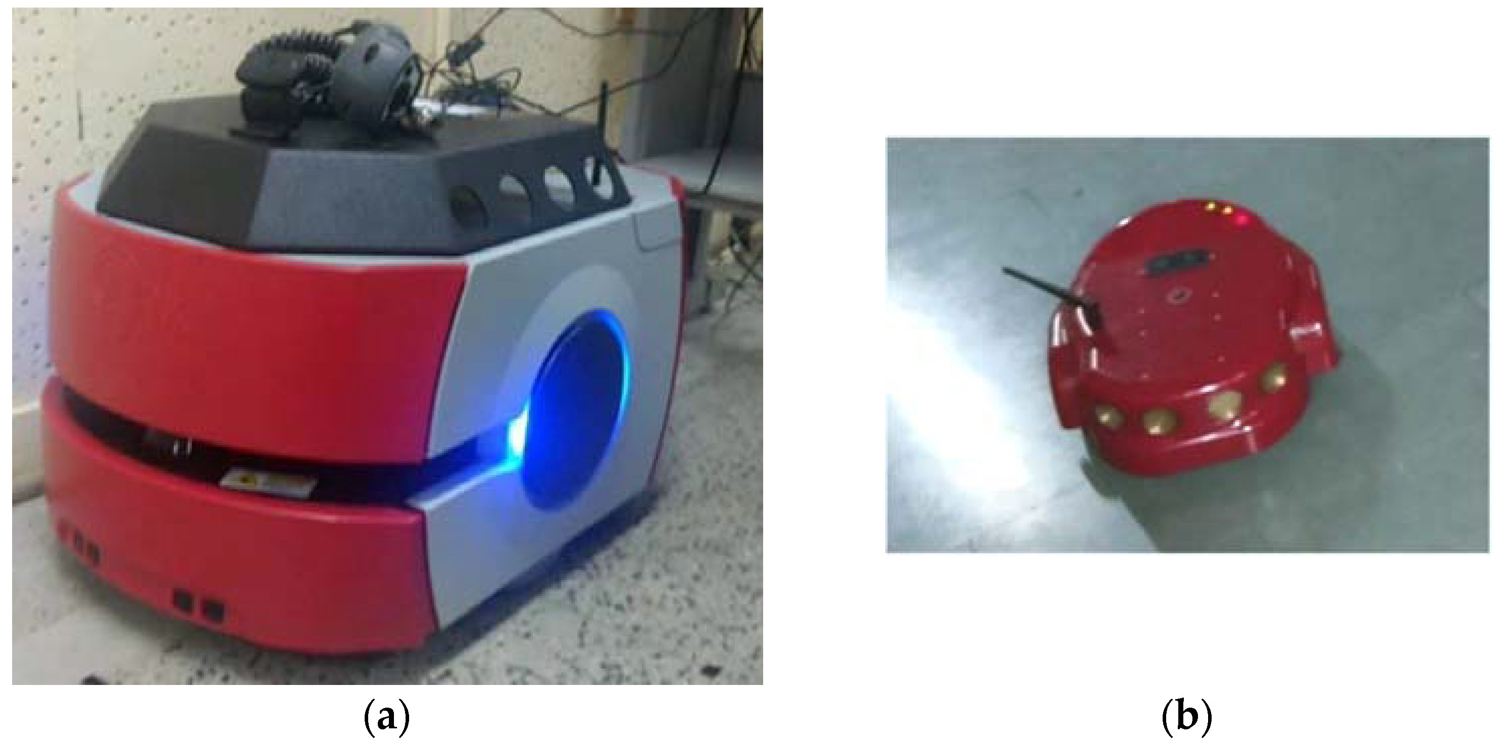
The mapping is done using a Pioneer LX robot, which is shown in Figure 5a. The robot itself cannot be used for display of chaining behaviour as the robot is extremely expensive and affording numerous copies of the robot does not make any practical application. The robot has a LIDAR system installed that can be used to effectively create a map that has to be used later. Thus, it aids the smaller robots to carry out the tasks they were required to do. For the actuation, we use robots that have much smaller dimensions, named the Amigobot, as shown in Figure 5b.

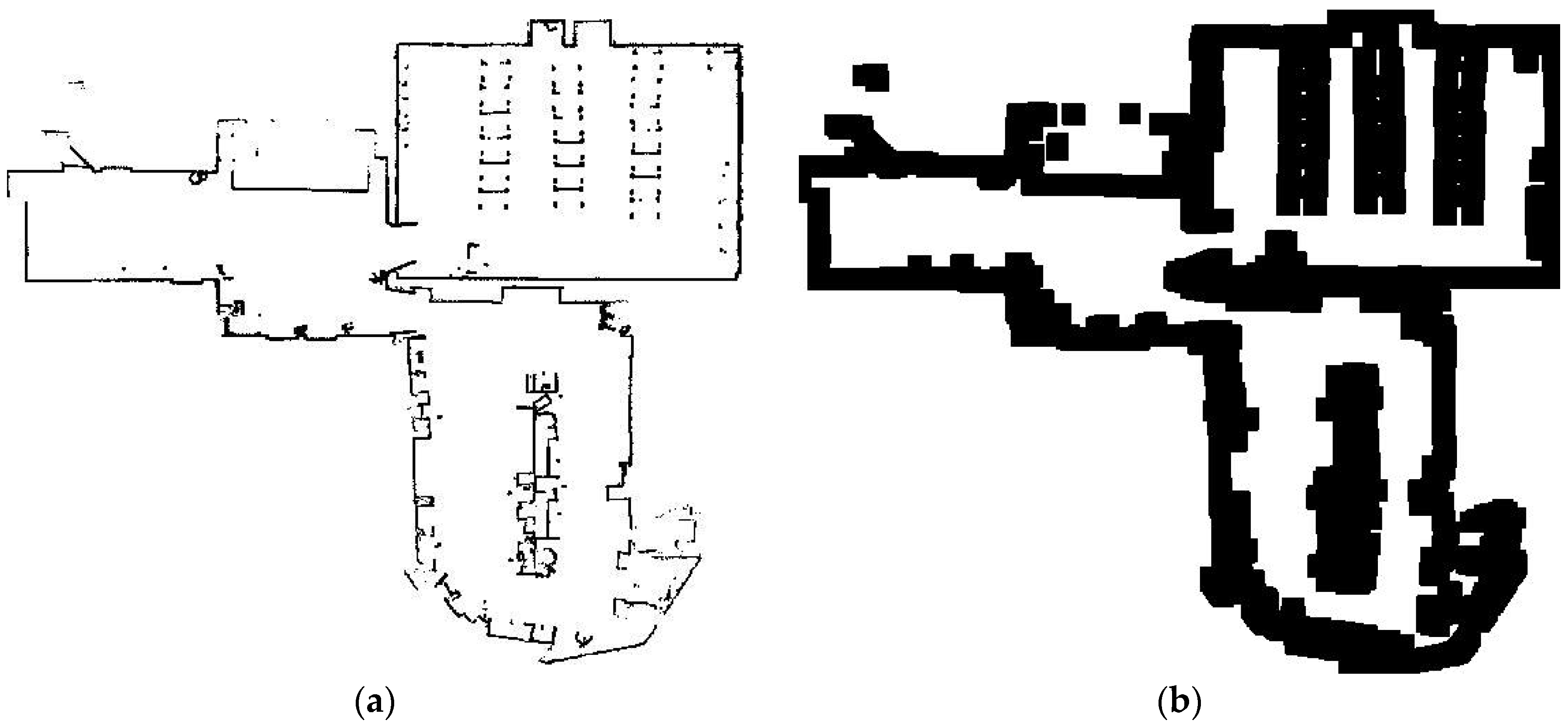
The robot has high resolution IMU and encoders through with indicative position of the robot can always be known, subjected to knowing the initial position. This makes the motion model of the filter used for tracking the robot pose. The robot’s sensor readings record measurements that can be used as the measurement model to correct the position estimates by using filtering. The robot hence continuously estimates its position. Knowing the position, the obstacle corresponding to every laser reading can be projected on an occupancy grid to make a grid map. The map so produced is post-processed to remove noise and regularize the obstacles.

During the post processing, any stray black pixels are removed. Then, all the boundaries are thickened. This is done so that the path obtained via A* algorithm is not too close to the actual boundaries. This helps by leaving a margin between the robot and the boundary in any case in the A* algorithm, thus giving a more practical solution.

4.2. A* Algorithm

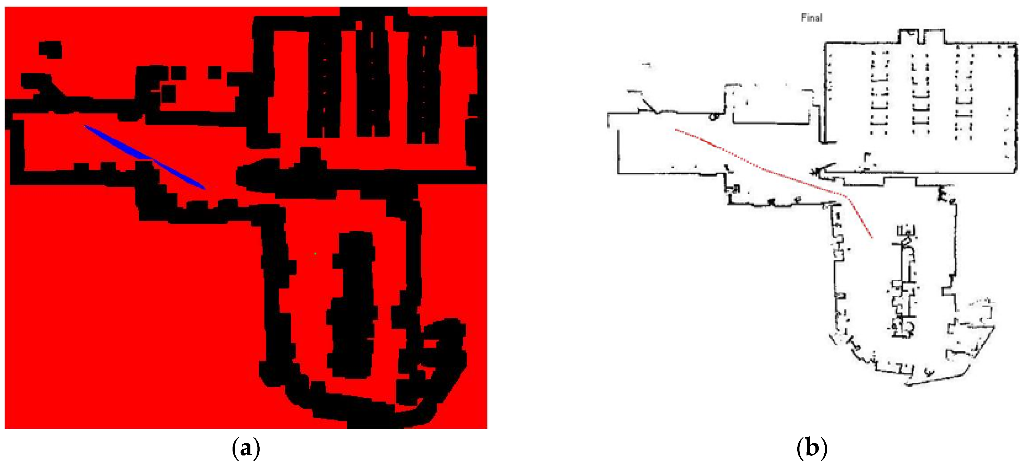
This algorithm helps us obtain the shortest path (τ_A) between the source (q_S) and the goal (q_G) in the given map. Since the robot is circular with radius R, the configuration space (C) can be obtained by inflating all obstacles by R. Free configuration space (C^free) consists of all configurations wherein the robot does not collide with any obstacles (C^free = C/C^obs, where C^obs is the set of configurations where the robot collides with an obstacle). The path τ_A: [0, 1] → C^free, is a sequential specification of configurations, starting from the source τ_A(0) = S, ending at the goal τ_A(0) = G, such that every intermediate point is collision-free, τ_A(s) $\in$ C^free, 0 ≤ s ≤ 1. The sub-script ‘A’ is used to emphasize that this is not the final trajectory of the robot.

A* algorithm is preferred over Dijkstra’s algorithm as this gives faster results. The A* algorithm uses Heuristic. The Heuristic used here is Euclidian distance (d(n, n’))which is both admissible and consistent in the given scenario. The map is discretized by filling in cells and each cell corresponds to the vertices of the graph. Every vertex n is connected to the 8 nearest neighbours that make the edges of the graph, making the neighbourhood function δ(n).

At each point of the execution, the algorithm aims to pick up a neighbour of a current node that promises the shortest distance to the goal. The expected distance from source to goal via a given point n is called as the total cost f(n) and is given by as the sum of current calculated distance (g(n)) and the heuristic value form current node to goal (h(n)). A queue of nodes is presented along with a bookkeeping sets Open used to store all nodes in the queue to be processed and Closed used to store all nodes which have been processed. The parents π(n) are saved for each value, and the parents are saved in a recursive manner for the final path found. This path is later accessed by the master robot to move. Algorithm 1 discusses finding path between starting and goal configuration using A* algorithm.

Algorithm 1: A* Algorithm

Input: Configuration Space (C), Source (S), Goal (G)

Output: path τA

FOR all cell c in Cfree

h(c) ← d(c,G), g(c) ← ∞, f(c) ← ∞

END

g(S) ← 0, f(S) ← h(S)

found? ← false

Q← empty priority queue prioritized by f(n)

Closed ← empty set, Open ← empty set

Enqueue S in Q

Add S in Open

WHILE Q is not empty

n = Top element in Q

IF n = G

found? ← true

Calculate τA using π

Break

END

Dequeue n from Q

Remove n from Open

Add n to Closed

FOR all n’ $\in$ δ(n)

IF n $\in$ Cfree ∧ n ∈ Closed

Add n’ in Open

Enqueue n’ in Q

c ← g(n) + d(n,n’)

IF c<g(n’)

g(n’) ← c, f(n’) ← g(n’) + h(n’)

END

END

END

END

IF found? = False

Return NULL

ELSE

Return τA

END

4.3. Potential Field Approach

This approach is used to obtain a path τ while avoiding the obstacles that come along the way. The algorithm assumes that the obstacles exert a repulsive force and the goal exerts an attractive force on the robot. This results in the area being converted into a series of potential highs and lows. The robot always tends to move towards the lower potential in an attempt to stabilise itself better. The robot here decides the placement and orientation of the co-ordinate system. The sum of all the forces acting on the robot decides the net force on the robot, thus deciding the next position where it should be. The algorithm moves the robot toward the goal until it reaches within the acceptance threshold of ε.

The obstacles are sensed by the robot using its sonar sensors. Hence, only those obstacles are taken that are within the sensing range and visibility of any of the sonar sensors. Further, the robot always knows its location q using localization modules or dead-reckoning calculations. The sub-goal g is supplied to the robot. It may not be the final goal of the robot but an intermediate goal for reasons discussed in Section 4.4. Algorithm 2 discusses robot control using potential field method. The algorithm uses potential field to calculate the force based on which the position of an ideal constraint-free robot is computed. This acts as the reference for the physical robot that uses a proportional controller for its motion. The algorithm assumes a collection of sonar sensors, such that the ith sonar sensor records a distance of d_i from the obstacle, while the sensor is placed at an angle α_i with respect to the robot. The repulsive force hence calculated is transformed from the robot frame of reference to the global frame of reference by multiplication of the rotation matrix. The robot has an orientation of q_θ and hence the rotation.

Algorithm 2: Artificial Potential Field based Navigation

Input: acceptance threshold (ε), sonar readings di, Goal g

Output: Path traced by the robot τ

Algorithm 2: Controller

WHILE d(q,g) < ε

q ← Position by localization

q’ ← APF(q)

θe = AngularDifference(q’θ − qθ)

v ← k1p d(q,q’)

ω ← k2p θe

END

Algorithm 3: Artificial Potential Calculation APF (q)

Calculate Fatt using Equation (2) using goal g

Frepel ← 0

FOR each sonar reading di on robot

${\mathrm{F}}_{\mathrm{rep}}^{\mathrm{i}}=\{\begin{array}{c}\mathsf{\eta }\left(\frac{1}{{\mathrm{Q}}^{\ast }}-\frac{1}{{\mathrm{d}}_{\mathrm{i}}}\right)\frac{1}{{\mathrm{d}}_{\mathrm{i}}^2}.\widehat{\mathrm{u}}\left({\mathsf{\alpha }}_{\mathrm{i}}\right), {\mathrm{d}}_{\mathrm{i}}\le {\mathrm{Q}}^{\ast }\\ 0, {\mathrm{d}}_{\mathrm{i}}>{\mathrm{Q}}^{\ast }\end{array}$

Frepel ← Frepel + Firep.R(qθ)

END

F ← Fatt + Frepel

q’x,y ← qx,y + F

q’θ ← tan−1(Fy,Fx)

return q’

END

4.4. Control for Master Robot

The above techniques are used to display a chaining behaviour, which is divided into two parts: motion of the master robot discussed in this section and the motion of the slave robot discussed in Section 4.5. The motion of the master robot requires two concepts, the first is navigation using a fusion of deliberative and reactive planning, and the second is being the leader of a fleet of robots. For the same of clarity, let us assume that all robots are numbered 1, 2, 3, and so on, starting from the master robot numbered 1. The positions are thus given by q₁, q₂, q₃, and so on. Each robot computes its position using its own localization system that is communicated to the necessary robots using inter-robot communication.

The deliberative approach represented by A* algorithm and reactive approach represented by the potential field algorithm are both fused to find an optimal path at the run time. This is done by using a ghost robot that follows the A* algorithm. This robot acts as the goal (g) for the potential field algorithm. Whenever the robot sees a distance from obstacle as less than d_APF, it shifts to a purely potential based reactive algorithm and when the robot sees no obstacle around, it transfers to motion using the A* algorithm using a ghost robot following control paradigm. This is the switching logic between the two algorithms. The potential field detects all objects at a small distance as obstacles and tries to overcome them. This module is used for controlling the movement of the master robot that acts as the main robot for the robot following it and is the leader in the chain of robots.

The path τ_A with smallest distance has already been calculated using A* algorithm using Algorithm 1. This path is strictly followed by the ghost robot. The ghost robot does not have to deal with any real-world obstacles and thus can follow the obtained path as it is. The master robot follows this ghost robot (g). If any obstacle is detected within a range of d_APF, it is treated as a new obstacle that was not taken into consideration during the creation of the static map, and the robot shifts to potential field mode. Now, the obstacles are treated as similarly charged to the robot, and the ghost robot (g) is treated as oppositely charged to the robot. This creates repulsion force between the robot and the obstacle and strong attraction force between the robot and the ghost robot. As soon as the robot is free from influence of the obstacle, the robot again starts following the ghost robot.

The ghost robot is made to travel the A* path (τ_A) that acts as the immediate goal for the robot. Suppose at any instance of time, the ghost robot is at a position τ_A(s), where s is the parametrization of the path in terms of time. To update the position of the ghost robot, we first find the closest position in τ_A to the current position of robot (q₁). The search happens in the local neighbourhood of s, denoted by δ(s), which is strictly positive as the ghost robot ideally only moves forward. The ghost robot further moves forward by a pseudo speed of v_F. This constantly pushes the robot to go ahead and follow the ghost robot. The ghost robot may be stopped from going forward if the distance between the actual and ghost robot is larger than a threshold η, which is effective if the actual robot is stuck or when the pseudo speed v_F is too large. This prevents the ghost robot from getting to far ahead from the master robot and helps the master robot follow the ghost robot easily. The ghost robot may also come back with a speed v_B if the main robot has a distance more than η for a time T. This is useful for avoiding situations wherein the robot gets trapped and cannot continue.

The chaining behaviour is implemented by adding additional forces to the navigation of the master robot. The master robot (q₁) is leading a chain with the immediately following child q₂. The following child exerts a force to the master robot. If the distance between the two robots is very large, an attractive force is exerted signalling the master robot to slow or move towards the child. Similarly, if the distance between the robots is too large, a repulsive force is generated to move the master robot in the opposite direction. The master robot may also be stopped if the distance between the master and following robot is more than a threshold Δ. This eliminates the chain from distorting, eliminates the group cohesion to be lost, and makes it easier for the slave robot to follow the master robot.

Algorithm 4 discusses motion control for master robot.

Algorithm 4: Leader Robot Controller

Input: Path obtained by A* algorithm (τA), position of follower robot (q2) and SONAR readings (di)

Output: Path traced by the robot τ

q1 ← qS1, s ← arg mins1∈δ(0) d(τA(s1),q1)

g ← τA(s)

reached? ← False

WHILE reached? = False

Get q1 from localization

Get q2 from inter-robot communication

Algorithm a: Get position of ghost robot

IF d(q1,g) > η

if t > T, s ← s-vB, else t ← t + 1

ELSE

S ← s + vF, t ← 0

END

Algorithm b: Force from the following robot

IF d(q1,q2) > ds

Ff ← Fatt(q2)

ELSE

Ff ← Frepel(q2).

END

Algorithm c: Other attractive and repulsive forces

IF di < dAPF for any di in sonar sensor readings

Calculate Fatt using Equation (2) using g as the goal

Frepel ← 0

FOR each sonar reading di on robot

${\mathrm{F}}_{\mathrm{rep}}^{\mathrm{i}}=\{\begin{array}{c}\mathsf{\eta }\left(\frac{1}{{\mathrm{Q}}^{\ast }}-\frac{1}{{\mathrm{d}}_{\mathrm{i}}}\right)\frac{1}{{\mathrm{d}}_{\mathrm{i}}^2}. \widehat{\mathrm{u}}\left({\mathsf{\alpha }}_{\mathrm{i}}\right), {\mathrm{d}}_{\mathrm{i}}\le {\mathrm{Q}}^{\ast }\\ 0, {\mathrm{d}}_{\mathrm{i}}>{\mathrm{Q}}^{\ast }\end{array}$

Frepel ← Frepel +Firep.R(q1,θ)

END

F ← Ff + Fatt + Frepel

q’x,y ← qx,y + F

q’θ← tan−1(Fy,Fx)

ELSE

Calculate Fatt using Equation (2) using g as the goal

q’x,y ← qi,x,y + F

q’θ←tan−1(Fy,Fx)

END

IF q = G1

reached? ← True

END

IF d(q1,q2) > Δ

v ← 0

ω ← 0

ELSE

θe = AngularDifference(q’θ − q1,θ)

v ← k1p d(q1,q’)

ω ← k2p θe

END

END

Send Term signal to all robots

4.5. Control for Slave Robot

This section is used for controlling the movement of the robot (q_i) that sees the robot ahead of it as the leader robot (q_i−1) and the robot following it as follower robot (q_i+1). Thus, the same robot acts as the leader for the robot behind and the follower for the robot ahead, forming a chain structure. Each robot of the chain follows this pseudocode.

Algorithm 4 helps multiple robots follow each other in a chain like fashion. The master robot follows the ghost robot and the slave robots follow the master robot one after the other. Potential based approach is used wherein the follower robot is attracted towards the leader, unless the distance between them becomes too small. The position of the robots is fetched from their localization modules and fed to the other robots via inter-robot communication. If the robot following this robot is more than Δ, the robot stops and waits for the follower robot to come closer before moving on. Algorithm 5 discusses motion control for slave/follower robot.

Algorithm 5: Slave Robot Controller

Input: position of master robot (qi−1), slave robot (qi+1), self (qi) and SONAR readings (di)

Output: Path traced by the robot τ

qi ← qSi

WHILE Forever

Get qi−1 from inter-robot communication

Get qi−1 from localization

Get qi+1 from inter-robot communication

Algorithm a: Force from the following robot

IF d(qi,qi−1) > ds

Ff ← Fatt(q2)

ELSE

Ff ← Frepel(q2).

END

IF di < dAPF for any di in sonar sensor readings

Frepel ← 0

FOR each sonar reading dj on robot

${\mathrm{F}}_{\mathrm{rep}}^{\mathrm{j}}=\{\begin{array}{c}\eta \left(\frac{1}{{\mathrm{Q}}^{\ast }}-\frac{1}{{\mathrm{d}}_{\mathrm{j}}}\right)\frac{1}{{\mathrm{d}}_{\mathrm{j}}^2}.\hat{\mathrm{u}}\left({\alpha }_{\mathrm{j}}\right), {\mathrm{d}}_{\mathrm{j}}\le {\mathrm{Q}}^{\ast }\\ 0, {\mathrm{d}}_{\mathrm{j}}>{\mathrm{Q}}^{\ast }\end{array}$

Frepel ← Frepel +Fjrep.R(qi,θ)

END

F ← Ff + Frepel

q’x,y ← qi,x,y + F

q’i,θ← tan−1(Fy,Fx)

END

IF d(qi,qi+1) > Δ

v ← 0

ω ← 0

ELSE

θe = AngularDifference(q’θ − qθ)

v ← k1p d(q,q’)

ω ← k2p θe

END

IF Term signal received and q’ = q

reached? ← True

END

END

4.6. Elastic Strip Model

This section is used to align the robots in a straight line. This line is the line between the first robot and the last robot. Thus, a virtual elastic strip is created between the first robot and the last robot. The intermediate robots act as pegs distorting the elastic strip. A force is exerted on the robots pulling them inwards towards the elastic strip.

Algorithm 6 helps the robots to align themselves in a linear fashion. This algorithm functions throughout the execution of the program, so that the robots always follow a straight line.

Algorithm 6: Elastic Strip Model

Input: Robot States (R)

Output: Expected Robot States (R’)

Strip ← Straight Line Between(rfirstposition, rlastposition)

FOR all robots r in R

Distance ← Euclidean distance between (rposition, Strip)

Force ← Distance * Fix_force

rforce = rforce + Force

END

5. Results

5.1. Mapping

The map with static features is first made using a 2D LIDAR and IMU sensors. Pioneer LX is used for the purpose. This is shown in the Figure 6. We perform robot mapping by logging the data recorded by the SICK LIDAR along with the odometry information of the robot. The key to creating good maps is to close the smaller loops before closing in the bigger as it results in the closing of the smaller loops and the poses belonging to the closed scan are fixed. Closing of smaller loops first result in smaller search spaces for detection of loop closures. Only after closing the previously detected loops should we go on to exploring new areas. After we have logged all the data, we perform processing on the raw data in order to register and clean up the map using the tool Mapper3 [24] developed by Adept Mobile Robots. The image obtained is then padded so that the path found does not get too close to the edges and remains in the practical limits of the robot following it.

Figure 6a shows the original map obtained with help of LIDAR. This map has sharp edges and shows the exact map of the area. Figure 6b shows the map after padding. A thick layer has been added to all the edges in order to make it appear as though all the areas where the robot’s centre can actually not be present is the part of the feature of the map from where the path should not be found.

5.2. Deliberative Planning

During deliberative planning, the use of A* Algorithm gives us the shortest path possible under given static map. This path is used as the primary path to be followed by the robot. A source and a goal position is given to the program to find the path between them using A* algorithm. This is done by searching the search space of the map while avoiding the obstacles. The process followed is shown in the figures below.

Figure 7a shows the working of the A* algorithm to find a path between the source and the goal. Figure 7b shows the final path obtained after the algorithm has run completely. It shows a path from source to goal in a dotted red line. Note that the path found stays away from all the edges in the original path. This is because a padded image was used during the process of finding the path.

5.3. Chaining

Here, the robots were asked to go from a pre-specified source to a pre-specified goal in a chain structure. As the slave robots’ sensors also detect the object ahead of them, i.e., their respective master robots, it has to be made sure that they do not perceive them as obstacles. The method by which this is done is that the master robot exerts a higher attraction force than the object ahead exerts the repulsive force. This results in resultant attraction toward the master robot. The images from the actuation can be seen in Figure 8. The results are also supplied as Video 1.

Figure 8a shows the robots before they have started the motion. As seen from the figure, the robots are placed in chain-like fashion initially, so that each robot except the last robot has one slave robot, and each robot except the first robot has a master robot. The motion of the robot when it has not yet encountered any obstacle is shown in Figure 8b. As seen above, the robots follow each other in a perfect chain-like fashion. Figure 8c shows the robots avoiding the obstacle. The robots intelligently avoid the obstacle placed in the way while maintaining the chain-like formation among themselves. Figure 8d shows the robots successfully avoiding yet another obstacle that has been dynamically placed. The robots in Figure 8d do not depict a chain formation. However, in Figure 8e, it can be seen that the robots have gained the expected chain formation back. Figure 8f shows the robots reaching the goal. The final position of the master robot is same as the goal marked in the map while finding the path using A* algorithm. However, the slave robots have their final position slightly away from it so as to avoid collision. These points are not predetermined and are solely fixed based on the potential field generated by the robots themselves. This results in a dynamic equilibrium among the slave robots.

5.4. Linear Arrangement

After applying the elastic strip model on the above suggested technique, the robots now move in fashion that almost always maintains a linear arrangement. The robots now align themselves linearly. The expected line is the one between the first robot and the last robot. Other robots are now placed on a line formed between these two robots. However, there are some slight deviation at times. The reason for these deviations is discussed in detail in Section 6.3.

6. Challenges

6.1. Equipotential Regions

There arise situations when the forces acting on particular robot are equal and opposite in nature. This makes the net force on the robot zero. The robot then behaves as if it is in an equipotential region. When such a case arises, a small tangential force is applied in the positive x axis direction of the robot. The value of this tangential force was calculated arbitrarily. This displaces the robot slightly, thus removing it from the equipotential region. Other solution to this problem is to constantly keep the robots in motion with a small linear velocity.

6.2. Increase in Number of Robots

Since all the processing is done by a central system, the increase in number of robots directly affects the performance of the system. According to the processing speed and capacity of the central system, this difference might not be noticeable until a particular number of robots is reached. In order to speed up the processing, parallel processing can be used up to some extent while calculating the position of the robots, but since every robot depends on the robot in front of it, this might prove a little difficult.

6.3. Linear Arrangement

The robots sometimes fail to follow a perfect linear arrangement while moving. This is due to the fact that, when the forces due to elastic strip are applied to the robots, it is assumed that those are the only forces acting on them. This makes the force calculation slightly faulty. Thus, sometimes the robots may not follow a linear arrangement due to this reason.

7. Computational Requirements

The robot used for map creation must have an accuracy enough so that the map created is fairly accurate. The sensors of the smaller robots should also be good enough to detect the obstacles at run time. The network over which the communication occurs needs to have a bandwidth support of a standard LAN connection (~10 Mbps). This network is used to transfer small chunks of data with high frequency. A central system of RAM 4GB is required for flawless execution of the algorithm for 4–5 robots. A processing speed of 3.4 Ghz works flawlessly in the above-mentioned conditions. As the number of robots increase, all the above-mentioned resources will have to be increased.

8. Conclusions

A source and goal is given to obtain a path via A* algorithm. This path is followed by the master robot, which avoids the obstacles using Potential Field Approach where the obstacles detected by sonar apply a repulsive force and the next point on the path previously planned applies an attractive force on the robot. The resultant of these two forces gives an acceleration to the robot that is used to determine its next position in the next time. The robot behind that, or follower robot-1, follows this robot by fetching its previous position and then using that as a goal and the other objects as obstacles. It again uses Potential Field Approach to determine its next position as described earlier. The same process is followed by the following robot-2 where it treats following robot-1 as its master. This process extends to multiple robots to help in move in chain-like fashion.

Furthermore, the algorithm assures that the robots move in a linear fashion. The desired straight line along which the robots move is the line created by the first and the last robot of the system.

Thus, it can be seen that the suggested approach can successfully be used to create a path planning algorithm for multiple robots that behave intelligently by following the shortest path and avoiding the obstacles that come in the way in a chained fashion. Thus, our algorithm is successfully able to demonstrate chained motion for a given set of mobile robots while avoiding obstacles.